
Introduction
Financial markets have the tendency to change their behavior over time, which can create regimes, or periods of fairly persistent market conditions. Investors often look to discern the current market regime, looking out for any changes to it and how those might affect the individual components of their portfolio’s asset allocation. Modeling various market regimes can be an effective tool, as it can enable macroeconomically aware investment decision-making and better management of tail risks.
In this Street View, we present a machine learning-based approach to regime modeling, display the historical results of that model, discuss its output for today’s environment, and conclude with practical use cases of this analysis for allocators.
Determining the Regimes
In order to understand how a portfolio might react to various regimes, one first needs to determine what the regimes are. There are different approaches to establishing regimes. One way is to specify regimes based on knowledge and experience in the markets. For example, one might categorize market regimes using “boom” and “bust” cycles, periods of high or low equity market volatility, changes in monetary policy, or “risk-on” versus “risk-off” sentiment, believing those to be good indicators of meaningfully changing market conditions.
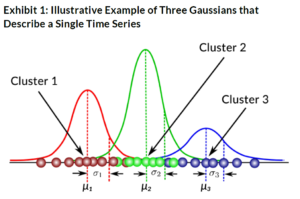
An alternative, more data-driven approach is letting historical data on assets and/or market risks delineate the regimes for you. A specific example of this approach is a Gaussian Mixture Model (GMM), which is a type of unsupervised learning method.1 The GMM uses various Gaussian distributions (another word for a normal, bell curve distribution) to model different parts of the data. As a simple example, imagine we had a single time series of an asset’s returns. As we know, returns of financial assets do not always follow a normal distribution. So a GMM would fit various Gaussian distributions to capture different parts of the asset’s return distribution, and each of those distributions would have its own properties, like means and volatilities. In Exhibit 1 below, we show an illustrative example of how a GMM might model a single time series. The green Cluster 2 captures the center part of the asset’s return data, while the red and blue Clusters 1 and 3 capture the tails.
Thus, the GMM is able to use a combination of normal distributions to model both the center and the tails of an asset’s distribution. We believe this is an especially helpful method for modeling financial assets, as their return distributions can often exhibit skew with a meaningful number of observations in the tails.
We want to provide the GMM with returns data from more than one asset to have a broader representation of the overall market and risks. So we will provide the GMM with the historical returns of the factors in the U.S. version of the Two Sigma Factor Lens, with most of the factor data dating back to the early 1970s (see Appendix 1 in the PDF version of this article for the start dates by factor). Instead of modeling the distribution of a single asset, like we did in Exhibit 1, we will ask the GMM to model the joint distribution of all 17 factors in the lens.2
Four Market Conditions
The result of the GMM using the Two Sigma Factor Lens factor data was four different clusters, or what we think may correspond to four different types of market conditions.3 As we mentioned earlier, regimes can be defined as periods of fairly persistent market conditions, so, in the next section, we will observe the behavior of these four market conditions over time to identify regimes.
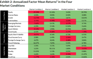
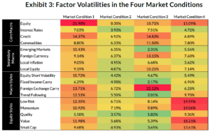
But first, what are these four market conditions? Each market condition from our GMM is characterized by a 17-dimensional Gaussian distribution (to account for the 17 factors in the Two Sigma Factor Lens). Each market condition’s Gaussian distribution has different factor means and volatilities, which are displayed in Exhibits 2 and 3 respectively, as well as correlation structures.4
One of the advantages of the GMM approach is that it is entirely data-driven—that is, the model outputs various market conditions, but that doesn’t tell us what those conditions are intuitively, and they won’t necessarily map exactly to well-known market environments that we or others could have specified ex-ante. This is both bad and good. Bad in the sense that it might be hard for us to put intuition behind the resulting market conditions, and good in the sense that it will hopefully tell us something that we wouldn’t have known without employing a technique like machine learning. After all, if we perfectly knew the market conditions without bias, why would we use relatively complicated models like GMMs?
So, again, while we don’t know exactly what these market conditions are capturing because they were generated by data and a model, we can imply what each represents by examining the factor behavior in each. Let’s attempt to classify and describe each.
Market Condition 1: Crisis
Market Condition 1 is likely one of the more interesting types of market conditions to investors when building portfolios, and we’ll spend the most time describing it. In this market condition, we see that several of the core and secondary macro factors exhibited extremely poor performance on average. For example, we observe that this was the only market condition where the global Equity and Credit factors had negative mean returns, and meaningful ones to boot. The Emerging Markets factor, which captures the risk-adjusted difference between emerging and developed markets, also averaged a negative return. This means that emerging markets struggled more than their developed counterparts. At the same time, the Local Equity factor averaged a positive return, indicating U.S. equity markets outperformed global markets on a risk-adjusted basis. Finally, the Equity Short Volatility factor was negative; this factor underperforms when equity market volatility is high.
The Interest Rates factor, representing global sovereign bonds, exhibited a positive mean return, perhaps demonstrating that investors flocked to lower-risk securities during this type of market condition. (This hypothesis is also supported by the positive mean returns of the Low Risk and Quality long-short equity style factors.) The Local Inflation factor, which attempts to capture the returns of an inflation hedge, was negative, indicating that U.S. inflation hedges didn’t pay off during these periods, as there was likely lower demand and economic activity when equity markets were in crisis.
In terms of the style factors, the equity styles exhibited mostly positive average performance, with the exception being Small Cap, indicating that larger cap companies do better in this market condition. Periods like this, in which overall equity markets are in “crisis mode,” could affect the viability of a small cap company more than a larger one, as worsening economic conditions are associated with a systematically larger decline in sales and investment for smaller firms than larger firms.6 We also see that the Trend Following macro style factor exhibited a large positive return; any directional trend in macro markets will benefit this factor, no matter whether the trend is up or down.
Finally, Market Condition 1 exhibited the highest average absolute correlation between the factors, although it was still very close to zero. This is by design, as the factors are constructed to be lowly correlated with one another, especially over long periods. However, we do observe factor correlations rising during shorter, crisis-like periods in both this analysis and others that we’ve run in the past,7 though the factor correlations don’t rise to the extreme values seen in unresidualized asset classes.
Based on all these observations, we believe the most appropriate label for Market Condition 1 would be Crisis.
Market Condition 2: Steady State
Market Condition 2 seems to cover the most normal and healthy market periods, as there are no obviously large drawdowns for any factor. Equity, Credit, and nearly every style factor performed well on average. We see that the mean returns for the Local Equity and Emerging Markets factors were nearly flat, indicating that the U.S. and the rest of the world experienced similar risk-adjusted returns. Finally, the Local Inflation factor exhibited a small positive mean return, indicating minimal benefit to a U.S. inflation hedge.
We’ll refer to Market Condition 2 as Steady State.
Market Condition 3: Inflation
In Market Condition 3, the U.S.-specific Local Inflation factor exhibited a double-digit mean return, the highest mean return for that factor across the four market conditions. This suggests that U.S. inflation hedges were generally rewarded in Market Condition 3.
We find that the global Equity and Interest Rates factors have small positive mean returns, underperforming most, if not all, of the other four market conditions (positive inflation shocks tend to be negative for both stocks and bonds). Additionally, central banks might combat higher inflation with higher interest rates, which would also serve as a headwind for bonds.
We see that the Foreign Currency factor exhibited the highest average return of any factor in this market condition, indicating that the USD underperformed G10 currencies on average. Inflation erodes purchasing power and therefor would be expected to coincide with a weaker local currency.
Based on the notable performance of the Local Inflation factor, we’ll call this market condition Inflation.
Market Condition 4: Walking on Ice
Market Condition 4 tends to occur around Crisis (and Steady State) periods,8 potentially indicating market fragility. Global equity markets (as proxied by the Equity factor) do well here, but with a higher volatility than their long-term average. In fact, the Equity factor exhibited its second highest volatility in Market Condition 4 (the highest was in Crisis, Market Condition 1). And more generally, factor volatilities were on average 1.6 percentage points higher in this market condition than their respective long-term averages.
We also find that most equity style factors’ mean returns were above average, with the main exception being Momentum. Additionally, these factors in particular experienced much higher volatilities compared to their long-term averages (e.g., Value exhibited 18.2% volatility in Market Condition 4 vs. 8.9% long-term; Momentum 19.1% in Market Condition 4 vs. 10.5% long-term; Low Risk 20% in Market Condition 4 vs. 10.4% long-term). This might mean that there is reversal behavior occurring within stocks exhibiting more choppy returns.
Overall, it looks like this market condition potentially captures risk-on market periods where bubbles might exist or be forming. We’ll label it Walking on Ice (WOI).
Historical Analysis of the Four Market Conditions
Now that we have an understanding of the various market conditions, let’s look back through history to see when each occurred. This analysis will be able to tell us the extent to which there have been fairly persistent market conditions, or regimes, throughout history.
For any given historical period, the GMM will estimate probabilities that the market was in the four market conditions. So each market condition will have a probability for a particular period, and the four probabilities will sum to 100%. Exhibit 4 shows the highest probability market condition for periods throughout history. We should note that each period displayed in Exhibit 4 is independent and identically distributed. This means the GMM evaluates each period completely independently, without awareness of what market conditions occurred in the past or future.
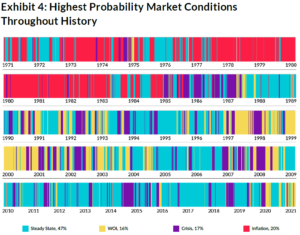
The legend at the bottom of the exhibit includes the percent of time the GMM found that market condition to have the highest probability over this 1971 – 2020 period. Steady State occurred most frequently since 1971, and each of the other three market conditions occurred in roughly 15-20% of the periods.
Starting from the top of the exhibit, Inflation was present exclusively in the 1970s and 1980s, as expected, since that period was characterized by relatively high inflation and interest rates. Over that first decade and a half, Inflation was fairly persistent (i.e., limited interruption from other market conditions), as it took quite a bit of time to get soaring prices for goods and services under control. We don’t see Inflation at any point in the last decade. Perhaps it will enter the picture in 2021 or 2022 if inflation does not prove transitory (more on that in the next section).
WOI occurred mostly during the tech bubble in the late 1990s and early 2000s. Markets were fragile for a while, as the bursting of the tech bubble occurred over multiple years. There were a handful of Crisis periods during this time as well, which correspond to days where the market had relatively large drawdowns, while the WOI periods were times where the market either temporarily reversed and/ or experienced large volatility. WOI was also the highest probability market condition in the immediate post-crisis performance reversals after the Global Financial Crisis (GFC) and COVID market crises, indicating that the market was recovering but still in a fragile state.
As expected, Crisis occurred during notable periods like the stock market crash in 1987, the GFC in 2008, and the COVID market crisis in 2020.
We find that Steady State dominated the last decade with a sprinkling of short-lived Crisis and WOI periods. This period coincided with the “decade of the central bank” where the Federal Reserve and its counterparts around the world exhibited major influence over the economy and markets. Over this time, Steady State was interrupted here and there by some Crisis flare ups (e.g., European Sovereign Debt Crisis in the early 2010s and the Taper Tantrum in mid- 2013), but the central banks would often step in to steady the markets through quantitative easing and rate cuts, rarely allowing WOI periods to form and returning markets to Steady State.9
To wrap-up and bring this back to regimes, we can certainly discern patterns of fairly persistent market conditions in Exhibit 4 (e.g., Inflation in the 1970s and 1980s, WOI in early 2000s, and Steady State in the recent decade). However, it was rare for one market condition to go for long periods without interruption from another. Transient themes can enter the picture on a short-term basis, and market conditions can change rather rapidly (think COVID market crisis in February and March 2020, followed by a sharp rebound). The GMM was reactive to those changes, resulting in abrupt market condition switches at times.
Where We Are Today
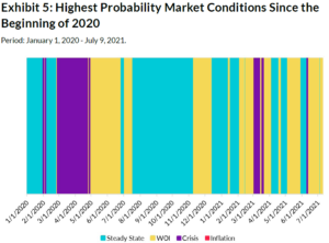
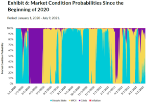
Now let’s use this model to understand market behavior over the past ~1.5 years. Exhibit 5 is an updated, “zoomedin” version of Exhibit 4, displaying the highest probability market condition in each period since the beginning of 2020. We provide additional detail on each market condition’s probability over the same period in Exhibit 6.
We find that Crisis was expectedly present in the COVID market crisis in February and March 2020, followed immediately by WOI. In the second half of 2020, Steady State was the predominant market condition. Then, in 2021, we observed a shift toward WOI, which as we mentioned earlier, might be a proxy for market fragility. Crisis entered the picture sporadically since then, most notably in early to mid-March 2021.
Finally, Inflation’s probability has been zero over this period (the maximum daily probability was only 0.01%), which is a particularly interesting result given the market’s fears of higher inflation and the high CPI prints in May and June 2021.
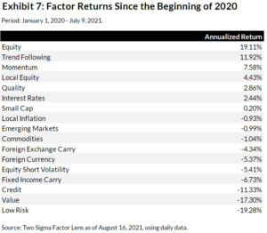
To explore this result further, in Exhibit 7 we display the factor returns since the beginning of 2020 and find that the factors that outperform the most in Inflation (Local Inflation and Foreign Currency) were negative.
We should also comment that the current period might be inflationary, but different from what we saw in the 1970s and 1980s (where Inflation showed up the most in our training period). Additionally, this model is not predictive, so we are not able to say whether Inflation will be increasingly important later in 2021 or the years ahead. However, stay tuned for future Street Views where we may provide updates on the model’s output.
Conclusion: Applying This Analysis to Investment Decisions
One way to approach modeling regimes is to determine them based on experience and knowledge of the markets. An alternative approach (and one that Two Sigma generally takes when solving problems) is more data-driven in nature. The unsupervised learning method presented in this Street View can add value by letting a large amount of historical data determine the regimes for you. The output of this model applied on the factors in the Two Sigma Factor Lens was four clusters, or market conditions. We then labeled those market conditions, based on the properties of each, as follows: Crisis, Steady State, Inflation, and Walking on Ice (WOI). We analyzed their behavior throughout history to identify regimes, or periods where market conditions showed some persistence.
We believe there are multiple use cases for allocators looking to apply this type of analysis. One use case is risk management. Allocators can enhance their scenario analysis by sampling from the distributions of these market conditions to stress test their portfolios.
Another use case is assistance with asset allocation decisions. Predicting market returns over long periods is difficult even under very stable market conditions. The evidence of rather quickly-changing market conditions presented in this Street View makes adherence to those long-term forecasts even more challenging. The implications for asset allocation might be that allocators should design portfolios that can withstand market condition volatility over the long-term, while potentially seeking opportunities for tactical shifts on shorter horizons.