Convolutional Neural Network Coupled with a Transfer-Learning Approach for Time-Series Flood Predictions


1
Institute for Rural Engineering, National Agriculture & Food Research Organization (NARO), 2-1-6 Kannondai, Tukuba City, Ibaraki 305-8609, Japan
2
ARK Information Systems, INC, 4-2 Gobancho, Chiyoda-ku, Tokyo 102-0076, Japan
*
Author to whom correspondence should be addressed.
Water 2020, 12(1), 96; https://doi.org/10.3390/w12010096
Submission received: 26 November 2019
/
Revised: 23 December 2019
/
Accepted: 23 December 2019
/
Published: 26 December 2019
(This article belongs to the Special Issue Machine Learning Applied to Hydraulic and Hydrological Modelling)
Abstract
:East Asian regions in the North Pacific have recently experienced severe riverine flood disasters. State-of-the-art neural networks are currently utilized as a quick-response flood model. Neural networks typically require ample time in the training process because of the use of numerous datasets. To reduce the computational costs, we introduced a transfer-learning approach to a neural-network-based flood model. For a concept of transfer leaning, once the model is pretrained in a source domain with large datasets, it can be reused in other target domains. After retraining parts of the model with the target domain datasets, the training time can be reduced due to reuse. A convolutional neural network (CNN) was employed because the CNN with transfer learning has numerous successful applications in two-dimensional image classification. However, our flood model predicts time-series variables (e.g., water level). The CNN with transfer learning requires a conversion tool from time-series datasets to image datasets in preprocessing. First, the CNN time-series classification was verified in the source domain with less than 10% errors for the variation in water level. Second, the CNN with transfer learning in the target domain efficiently reduced the training time by 1/5 of and a mean error difference by 15% of those obtained by the CNN without transfer learning, respectively. Our method can provide another novel flood model in addition to physical-based models.
1. Introduction
The East Asian regions along the North Pacific have recently experienced an increase in catastrophic flood disasters due to larger and stronger typhoons. To reduce and mitigate flood disasters, artificial neural network (ANN) models may be a beneficial tool for accurately and quickly forecasting riverine flood events in localized areas [1], in addition to conventional physical models [2]. In Japan, areas vulnerable to strong typhoons and heavy rainfall events have experienced severe riverine flood disasters in the last 3–4 years [3]. An overflow-risk warning system that is based on real-time observed data has been successfully working for most major rivers in Japan. However, a flood warning system that can forecast with a quick response has not been practically implemented in specific locations of rivers. If the specific time and location of inundation were forecasted by the flood warning system before the inundation occurred, most people may have been able to evacuate these locations in past flood disasters. Consequently, the number of victims may have been reduced. When a forecast flood warning system is developed for practical use, an ANN model with deep learning is a candidate due to the model’s features. The ANN model is a data-driven model that does not need physical-based parameter setups unlike physical models. For example, a rainfall-runoff model should be calibrated, using numerous parameters that are based on complex physical laws in a target watershed [4]. Like the rainfall-runoff model, the setup of a physical model requires heavy work. The ANN model can predict a near-future trend that is based only on the learning of past data. ANN prediction usually has a low computational cost, although the learning incurs high computational costs. The major beneficial uses of the ANN-based flood model are related to a quick response to symptoms of a near-future flood event and an easy run using only past data [5].
Numerous studies of ANN models have been performed for flood predictions [6]. ANN models that adopt a deep learning approach have been recently employed in practical flood predictions [7]. As another type of ANN model, the long, short-term memory (LSTM) architecture [8,9] was utilized for water-level predictions during flood events [10,11,12].
In most case studies, ANN models successfully predicted past flood events with numerous datasets. In general, ANN models require high computational costs in the training process due to large datasets. To reduce the high cost of computational runs, our study introduces a transfer-learning approach [13]. The premise of the approach is that a model pretrained by large datasets in a source domain can be reused in other target domains. After retraining the part of the pretrained model with the datasets of the target domains, the retrained model can provide reasonable outputs with a low computational cost.
Our focus on flood events is to predict time-series data, such as water levels. The LSTM architecture implemented in an ANN model is the best tool for the treatment of time-series data. LSTM coupled with transfer learning has been developed. Laptev et al. [14] reported that their multilayer LSTM with transfer learning reduced errors more than LSTM without transfer learning in the long-term trends in electric energy consumption in the U.S. However, LSTM generally has not been successful especially for short-time, rapidly changing, and non-periodical data, such as data on flood wave. This finding can be explained as follows: An unknown value at a subsequent time step is rarely predicted from the present value because numerous temporal trends may exist [15].
A convolutional neural network (CNN) architecture [16] is primarily employed for two-dimensional (2D)-spatial image classification. The implementation of CNN in an ANN model achieved satisfactory performances with transfer learning in a variety of image analysis fields [17,18]. The ImageNet created by VGG16 [19], which uses 150 million images, is often employed to perform image classification for a new image dataset. CNN with transfer learning is successful because a CNN gradually structures from low-level visual features on a previous layer to semantic features that are specific to a dataset on a deeper layer [20,21]. Therefore, we considered that a CNN with transfer learning is more reliable and practical than a LSTM with transfer learning.
A technical challenge is to perform a conversion from time-series data to image data in an ANN model. Several studies have reported how to map time-series trends in a 2D spatial image. For example, stock market predictions in near-future trend employed the image of 31 stocks × 100 time steps [22]. The precipitation predictions utilized an image of spatial information of climates in time series, such as air temperatures at eight locations × eight time steps with a ten-minute interval [23]. If we apply these conversion techniques, the CNN coupled with a transfer-learning approach can predict time-series data for flood events.
This paper proposes a new data-driven-based model for flood modeling. The model consists of a CNN incorporated with transfer learning to efficiently and quickly predict time-series water levels in flood events even in different domains after pretraining the CNN in a certain domain. First, we will show the verification of the CNN-based flood model in large datasets obtained in a certain watershed. Second, we will evaluate the performance of the CNN with a transfer-learning approach in a different watershed. Last, we will evaluate the prediction accuracy for the number of retrainings of the CNN with the transfer learning.
2. Materials and Methods
2.1. Study Site
We selected two watersheds that do not have flood control facilities such as large dams and ponds (Figure 1). The first watershed is a part of the Oyodo River watershed, which is located in Southwest Japan. The watershed has an area of 861 km2, a main river with a length of 52 km that flows to the Hiwatashi gauge station near Oyodo River Dam (31.7870° N, 131.2392° E) downstream, and an elevation that ranges from 118 to 1350 m. The area often experiences heavy rainfall events from the summer to early fall due to typhoons. This watershed is named “Domain A” in this study. Another watershed is the Abashiri River watershed toward the northeast of Hokkaido. The watershed has an area of 1380 km2, a main river with a length of 115 km that flows to the outlet in the North Pacific, and an elevation that ranges from 0 to 978 m. Heavy rainfall events have seldom occurred due to weak monsoon impacts and few occurrences of typhoon tracks and approaches. We refer to this watershed as “Domain B”.
2.2. Data Acquisition
The hourly datasets for rainfalls and water levels from 1992 to 2017 in Domain A and 2000 to 2019 in Domain B were obtained from the website of the hydrology and water-quality database [24], managed by the Ministry of Land, Infrastructure, Transport, and Tourism in Japan (MLIT Japan) and the meteorological database [25] that belongs to the Japan Meteorological Agency (JMA). The observed datasets in Domain A were obtained from five gauge stations for water level and 11 gauge stations for rainfall. Domain B had four water-level stations and nine rainfall stations. The downstream stations where the model predicts water levels were Hiwatashi for Domain A and Hongou for Domain B (Figure 1). We focused on the historical flood events at each domain. Each flood event has a 123-hour duration, including the time of the flood maximum peak, three days before the peak, and two days after the peak. One maximum peak during the duration of each flood event was identified when the water level exceeded a certain criterion of water levels—approximately 45% to 60% of the highest peak of the observed datasets among all flood events. The quantity of data for each flood event is 123. If multiple peaks exist locally in one flood event, note that only the highest peak is regarded as the maximum value of the event. The datasets in Domain A and Domain B are listed in Table 1 and Table 2, respectively. The geographical and observational characteristics of both domains are shown in Table 3.
2.3. ANN and CNN Features
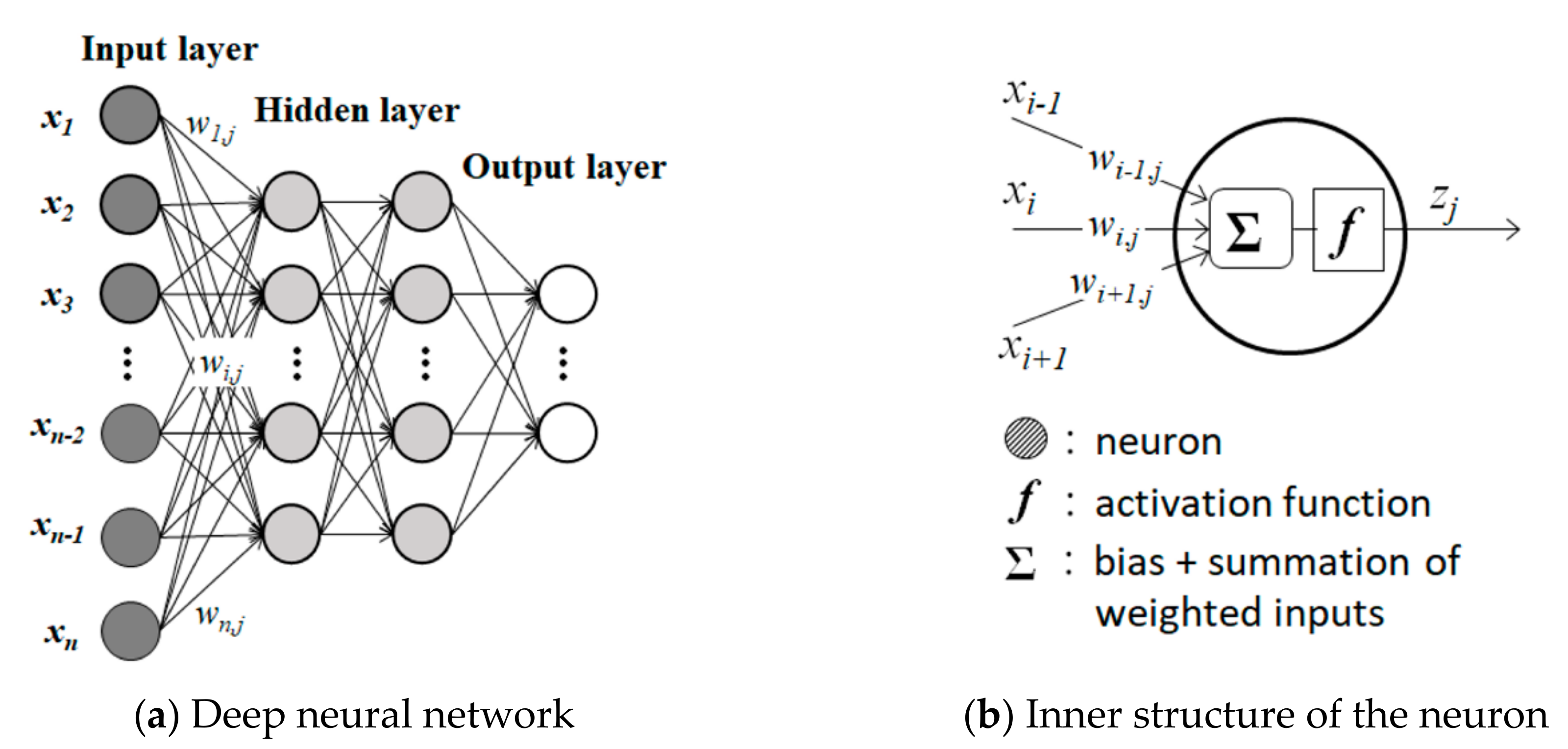
An ANN model usually consists of three layers—input layer, hidden layer, and output layer—and creates network with neurons. Note that the hidden layer often has multiple layers as a deep learning approach. Each neuron has an activation function that filters input values x with weighted coefficients w into an output value z. If a layer has n neurons, a certain neuron j in a subsequent layer receives n input values. These inputs weighted by coefficients are integrated and added by bias bj. The activation function f outputs zj from a neuron. These variables are defined in the following equations. The structure of the ANN model is shown in Figure 2.
A CNN is a type of ANN architecture with a deep-learning approach. We created a relatively simple algorithm of a CNN based on past studies [16,23]. The variables in Equations (1) and (2) are mapped to the 2D spatial image in the CNN, which consists of a convolution layer (convolution) and a max-pooling layer (pooling). We consider that the input variable x has L × L 2D source pixels, which is filtered with a H × H small window of convolution with a table of weighted values. The convolution takes the same size of values from the source image, and then multiplies the weighted values of the H × H window to the filtered values of source pixels. The filtering is repeated over the source image by shifting the window. Components of the input and filter are defined as xi,j (1 ≤ i ≤ L, 1 ≤ j ≤ L) and wk,l,n (0 ≤ k ≤ H − 1, 0≤ l ≤ H − 1, 1 ≤ n ≤ N), respectively. This process is shown in Figure 3. Note that a zero-padding technique was introduced to ensure that the size of input is equivalent to that of the output. The xi,j is multiplied by wk,l,n while separately shifting a grid at (i,j) on the filtering. This equation, including the convolution form and bias bn in the function, is expressed as follows:
We use a rectified linear unit (ReLU) as the activation function (f), which can select positive input values due to an improvement in the conversion of a matrix, as expressed in the following equation.
By filtering in the convolution, common features among images are extracted when the filter pattern is similar to a portion of each image.
The pooling does not have weighted coefficients and activation functions, is usually utilized to produce 2D data, and is defined in the following equation:
where Up,q is the square unit domain with the size R × R and (p,q) are the horizontal and vertical components. Up,q is moved on a 2D image with a non-overlap approach. As horizontal and vertical scales are shrunk 1/R times, the maximum value of xi,j,n in Up,q provides output with a data size of 1/R2 times of the input 2D data. The features extracted by the convolution can satisfy the consistency by means of the pooling even if the same features in reality are recognized as different features due to searching errors. Our CNN algorithm had two convolution layers and two pooling layers.
By performing these processes, smaller-size 2D image data are generated and then passed to a fully connected layer, which has the same function of Equations (1) and (2). These 2D image data are converted into numerous 1D digital datasets that involve information about classification of the original image. A softmax function is a normalized exponential function in Equation (7) that converts outputs to probability quantities in the output layer. It evaluates the binary classification.
However, our model prediction requires a specific magnitude of water level, instead of classification. Therefore, we introduced the sigmoid function into the softmax position to assign the magnitude from the normalized value (0 to 1) between the maximum value and the minimum value of the water levels.
2.4. Transfer Learning
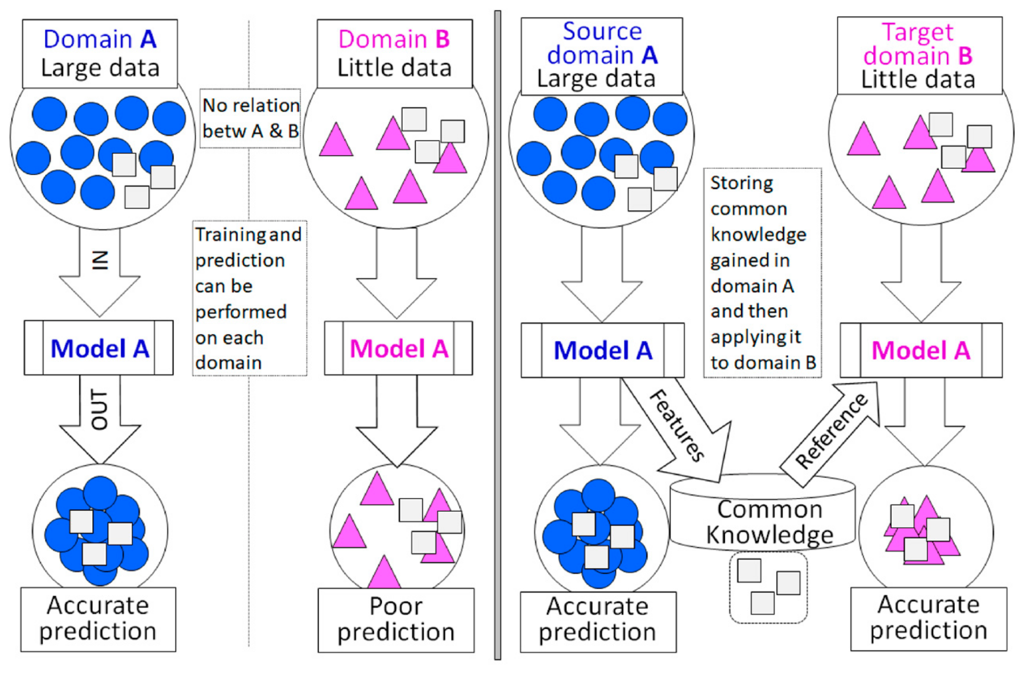
We assume that two domains exist separately. When a model is trained in a certain (source) domain with large datasets, it usually takes ample time to have an accurate prediction. If the model is applied to another (target) domain without any connection with the source domain, training it causes ample time. Transfer learning is one of the solution methods for improvement of the efficient prediction (e.g., reduction of run time) in the target domain [13]. The transfer learning can reuse common knowledge obtained from the source domain for the target domain. This overview sketch is shown in Figure 4. The CNN coupled with a transfer-learning approach (CNN transfer learning) is a recently successful method in image classification. As our model should perform time-series predictions, CNN transfer learning was utilized in this study by means of a conversion tool between time-series data and image data. First, the CNN was run in the source domain (Figure 5a). Second, parts of the hidden layers of the CNN were fixed and reused in the target domain. Last, “the fully connected layer 1” and “the fully connected layer 2” in the deep layers were retrained, using the datasets of the target domain (Figure 5b).
2.5. Data Conversion from Time-Series to Image
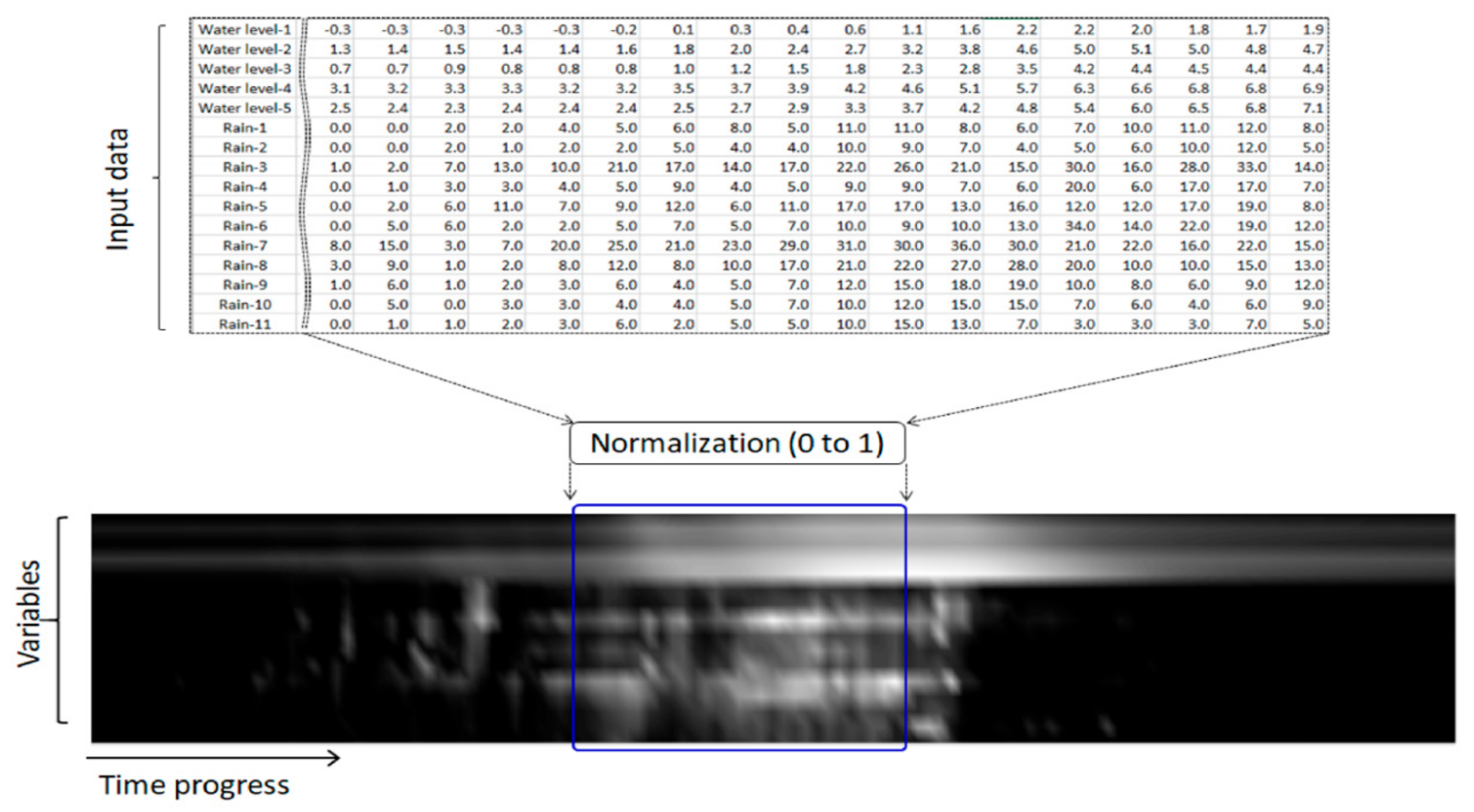
To perform time-series predictions with the CNN, a conversion method between time-series data and image data is necessary. As shown in Figure 6, our method was a simple way to arrange 16 variables (rainfall and water level) at all gauge stations from upstream to downstream on the vertical, and to arrange the temporal variation of each variable on the horizontal. The digital values were then converted to an image by using a black-and-white gradation that ranges from zero to one and is normalized by the maximum and minimum values of all observed datasets of water level and rainfall. The spacing between two values on the horizontal axis was one hour. The interval of the vertical axis was one for simplicity.
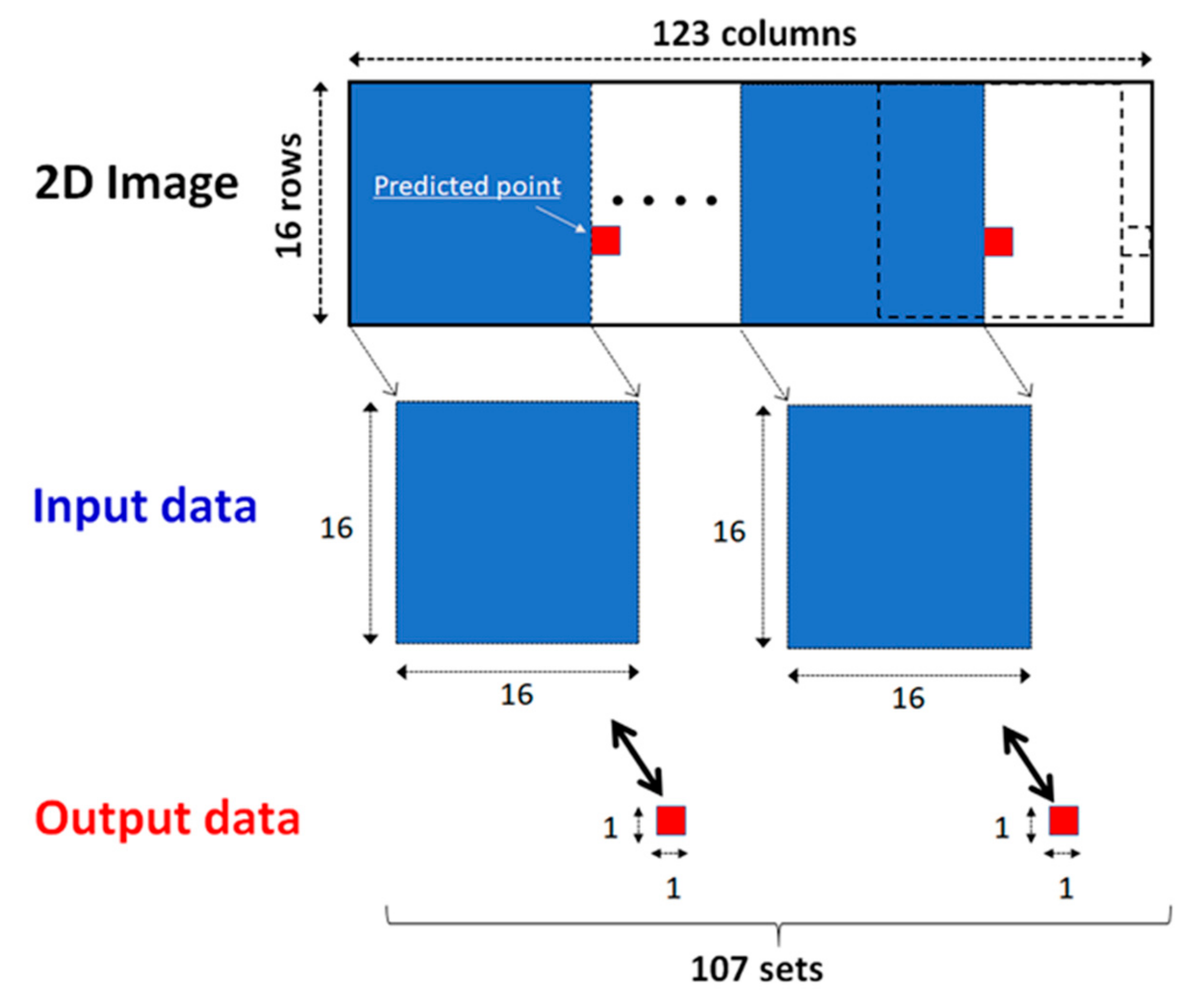
The image in the CNN has to correspond to a value of the water level in the time progress when train and prediction are conducted in the CNN. A 16 × 16 image was selected from the 2D image of a flood event due to the limited number of variables. A square image is used as input data. The information from the input data was associated with a 1 × 1 image (i.e., value) of the output data at the predicted point. We assumed that the flood-related information in a square image generates the value of the predicted point in the next time step (i.e., in an hour). Note that the predicted point indicates a location where water levels are predicted. This treatment was separately repeated in time progress as shifted from the head of the 2D image to the tail. Drawing information is shown in Figure 7. This data treatment was also employed when the LSTM predicts the value in advance using current and 15 past data values provided from 16 variables. The LSTM searches the relationship among plural line-based data; however, the CNN finds spatial patterns among 2D images.
The number of variables (i.e., four for water-level gauges and nine for rain gauges) in Domain B differs from that of Domain A. To make the image size of Domain B equivalent to that of Domain A, as shown in Figure 6, the image size has been expanded from 123 × 13 to 123 × 16, using the interpolation that maintains high-resolution images with the Lanczos algorithm [26].
2.6. Computational Setups in CNN and CNN Transfer Learning
Four cases were selected to evaluate the errors between predicted outputs and observed outputs in Domain A, using the CNN, and those in Domain B, using CNN transfer learning. These cases involved datasets that had the first-to third-position highest peaks in each domain (top three datasets) and two datasets with midlevel peaks, which were chosen among the other events in each domain. The four cases of the top three datasets and one midlevel-peak dataset were used as the datasets of the test process. Note that another midlevel-peak data set remains in the validation data set to evaluate at least one midlevel-peak dataset during the validation process. First, the CNN was trained with the training datasets, excluding the top three datasets and two moderate-peak datasets. Second, the trained CNN was checked to see whether a loss function shows overfitting, using validation datasets, including the top three datasets and the two datasets with moderate peaks as a representative of most datasets. This validation is usually performed to conduct a no-bias evaluation of a model. Last, a test was performed using one of the top three datasets or the moderate-peak dataset. In general, these procedures are usually utilized in machine learning [27,28]. In Domain A, we chose 38 events for training, four events for validation, and one event for testing (Table 4). Domain B had 12 events for training, four events for validation, and one event for testing (Table 5).
The programs for the flood models (CNN and CNN transfer learning) were created by Python (version 3.6.4) [29], incorporated with Keras libraries [30] on the Window-OS PC that has the Intel(R) Core(TM) i7-4770K CPU @ 3.50GHz. The setups of several parameters, such as batch size, epoch number, and activation functions, are shown in Table 6.
3. Results
We verified a typical classification by using the CNN as a preliminary examination, which is often used for image analyses based on “true or false” binary classification. The classification in this study was defined as upward or downward trends of water levels. The results showed a satisfactory accuracy rate of 88.8–93.5% for the cases from A1 to A4 (A1–A4) in the selected datasets of Domain A. However, the errors were caused by small up-and-down oscillations that primarily occurred during an early rising phase of a waveform. By this verification of the binary classification, our CNN can capture the upward and downward trends of flood waves. A detailed explanation is shown in Appendix A.
We also evaluated an effect of a pixel-size difference between an original image (123 × 13 pixels) and a resized image (123 × 16 pixels) in Domain B on CNN predictions of water levels. Predicted waveforms of the resized image in test datasets of the cases from B1 to B4 (B1–B4) were similar to those of the original image in another preliminary examination. However, the RMSEs obtained by the resized image are moderately reduced from those by the original image. Therefore, we assumed that the effect of the pixel-size difference could be limited to dramatically modify the CNN predictions of water levels. A detailed explanation is shown in Appendix B.
3.1. Verification of CNN Prediction With Source Datasets
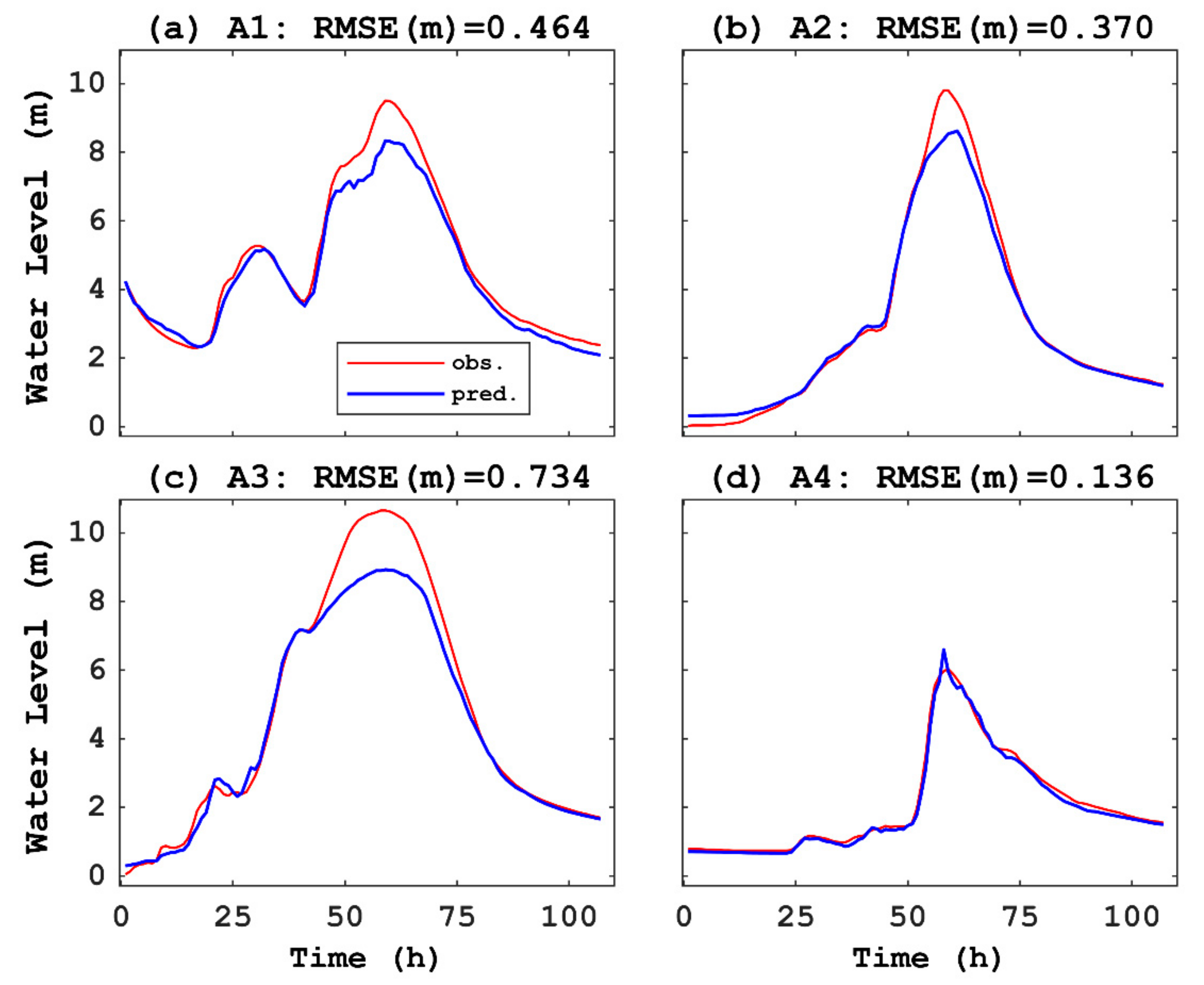
The CNN predicted the water levels of A1–A4 in Domain A after training the CNN among 38 flood events. To use the validation datasets for each case, including the top three datasets that have higher peaks of floods, the RMSEs ranged from 0.14 to 0.73 m, which corresponds to 2.6–6.9% of the variation between the minimum value and maximum value among the validation datasets. These errors can be acceptable because the top three datasets were excluded in the training process. In the test process for A1–A4, the CNN had an acceptable performance with a less than 10% relative error (Figure 8 and Table 7), although the higher peak of each A1–A3 prediction did not follow the observed peak. For example, the A3 prediction to capture the highest peak (3 September 2005) of flood wave shows that the RMSE was 0.73 and the relative error was 6.9%, although the peak height could not be captured by an approximately 20% difference (Figure 8c). For the dataset with the moderate peak of the flood wave (14 August 1999), the CNN in A4 predicted a considerably better shape of the water level, whose relative error was only 2.6% to the total variation in the water level during the 14 August 1999 event (Figure 8d). These results indicate that the moderate peak flood of A4 was typical for prepared datasets in the training process. Capturing a higher peak of each dataset of A1–A3 caused poor prediction due to exclusion of the A1–A3 datasets in the training process.
3.2. Verification of CNN Transfer Learning with Target Datasets in Domain B
After the verification of the CNN via the training, validation, and testing processes in Domain A, the transfer learning on the fully connected layers 1 and 2 was conducted in Domain B. The number of retrainings can be an important factor for improving the prediction of the CNN transfer learning. We evaluated how RMSEs are reduced based on the number of retrainings. Figure 9 shows the RMSEs for all cases (B1–B4), which are calculated by the observed and predicted water levels with respect to the number of retrainings. The number zero in the horizontal axis means that the CNN was employed without any retrainings in Domain B. As the number of trainings increased, the RMSEs for B1–B4 were reduced. The retraining converged approximately by approximately 20 times.
Figure 10 shows the comparison between the predicted water level and the observed water level in a time series during flood events in the test datasets of B1–B4 after the 20-time retrainings. These wave shapes tend to rise earlier than the observed wave that actually increased before the peaks. The predicted wave curves had small oscillations or non-smoothness.
In addition, the RMSEs of B1–B4 in the test datasets indicates 0.06–0.15 m, which corresponds to a variation from 3.3% to 4.3% between the minimum value and maximum value of the water level of each dataset (Table 8). The RMSEs are approximately equivalent to or reduced by at most 20% from those (0.06–0.20 m) of the CNN prediction with 100 trainings in Domain B, without transfer learning and with resized 123 × 16 pixels (Table 8). The retraining time of the CNN transfer learning was considerably shorter due to retraining the part of the CNN structure compared with the computational cost of the CNN without transfer learning. During the check process of the validation datasets after the 20-time retrainings, the RMSEs of B1–B4 ranged from 0.10 to 0.12 m, which corresponds to reasonable values from 2.6 to 3.2% for the variation between the minimum value and maximum value of the water level for each dataset.
4. Discussion
The time-series water-level predictions of A1–A4 using the CNN in Domain A showed acceptable agreement with the observed data, although the higher peaks of each of A1–A3 were poorly captured. Comparisons with other neural networks, such as the fully connected deep neural network (FCDNN) [7] and recurrent neural network (RNN) [31] indicated that our CNN prediction was poorer than the performance of these models. For example, Hitokoto and Sakuraba [7] reported that their FCDNN provided better predictions of water levels for the top-four largest flood events from 1990 to 2014 in the same watershed. The RMSE in an hour prediction of water level was 0.12 m, which is approximately 1/3 of the mean RMSE of our CNN prediction, due to the use of two different verification methods. The RMSEs of the FCDNN were calculated by the leave-one-out cross-validation method [32], in which three of the top four largest flood events were included as training datasets for each prediction. Our CNN excluded the top three datasets in the training process. Therefore, the accuracy of the CNN may not be worse than that of the FCDNN.
In addition to the flood prediction, the time-series predictions in other fields have been performed utilizing the CNN. Temporal predictions of the precipitation occurrence, as performed by the CNN, showed that the accuracy exceeded 90% in the first lead time based on the quadrant classification, which is based on the combination of yes and no occurrences in prediction and observation [23]. Another example of stock market prediction by the CNN that reported 50% accuracy was achieved in the upward or downward trend of 31 stocks [22]. Although the backgrounds and computational setups of these studies completely differ from those of our study, the preliminary numerical examination of the CNN predictions based on binary classification (i.e., upward or downward value of water level) achieved approximately 90% accuracy. Therefore, our temporal prediction by the CNN can produce high accuracy.
Our method uses the CNN coupled with a transfer-learning approach in time-series predictions. It may be original based on the literature review for machine-learning-based flood models in the latest two decades [33]. The results of the CNN transfer learning after 20-time retrainings show that the RMSEs were less than 5% of each variation in water level in the test dataset in Domain B. These errors are slightly reduced from those of the CNN in Domain A. However, some specific differences exist between the predicted water levels and the observed water levels in Domain B, which were not observed in the CNN predictions in Domain A. For example, the predicted flood peaks were slightly underestimated by only 5%–10% of the variation of observed water levels in B1–B3 (Figure 10). The slight underestimation of wave peaks in B1–B3 may be caused by the genetic tendency of the CNN trained in Domain A. This finding may be attributed to the notion that the CNN was substantially fitted to the flood waveforms that have steeper slopes of peaks.
Quantitative improvement in the CNN transfer learning appeared in the reduction of computational costs. The CNN transfer learning’s RMSEs are slightly reduced from those of the CNN without transfer learning (i.e., a single use of CNN) in Domain B (Table 8). The former had 20-time retrainings of “the fully connected layer 1” and “the fully connected layer 2” of the CNN, which means that the number of parameters of the training process was also reduced (Figure 5b). The latter required full training by 100 times (i.e., epochs = 100) through all layers of the CNN (Figure 5a). Based on our computer resources, the computational cost was reduced to approximately 18% compared with the CNN without transfer learning. Thus, the beneficial aspect from the results of the CNN transfer learning reveal that the computational costs were substantially more reduced than the CNN without transfer learning once the CNN is well verified in Domain A (source domain). The CNN has to first perform the pretraining. The CNN can be applied to other domains once the CNN is pretrained.
A few studies of time-series prediction have been performed by using the LSTM, with a transfer-learning approach. For example, Laptev et al. [14] successfully reduced the prediction errors in the target dataset of time-series electricity loads obtained from the US electric company, using transfer learning with multiple layers of the LSTM. For error evaluation, they reported that the symmetric mean absolute percentage error (SMAPE) in small-size datasets (till the maximum of 20% of the total datasets) in the target domain was improved by approximately 1/3 of the SMAPE for the total datasets. Their LSTM was likely to improve the accuracy even in small-size datasets with transfer learning. Although comparing our results is difficult due to different-types of datasets and different methods of error evaluation, the accuracy improvement in a target domain (Domain B) using transfer learning could be achieved with approximately 15% reduction in a mean error difference between the CNN with transfer learning and that without transfer learning in the first trial of our study. Note that the mean error difference is defined in the following equation:
where TL is with transfer learning, and NONTL is without transfer learning.
The CNN transfer learning in Domain B can be necessary to further reduce the RMSEs compared with those from a single use of the CNN without the transfer-learning approach. The RMSEs of CNN transfer learning can be smaller because the transfer-learning approach in this study was simple (i.e., retrainings only of the fully connected layers 1 and 2). In general, if some deeper layers close to the end of the CNN is retrained, the transfer learning can be more effective for improving predictions (e.g., Wang et al. [34]). For example, we may perfume the sensitivity tests of retraining the layers, such as the max-pooling 2 and the fully connected layers 1 and 2 (Figure 5a). Therefore, the next step of our study can perform the retrainings of additional layers in the CNN in Domain B.
5. Conclusions
We created a new model that consists of the CNN with a transfer-learning approach and a conversion tool between the image dataset and time-series dataset. The model can predict time-series floods in an hour in the target domain (Domain B) after pretraining the CNN with numerous datasets in the source domain (Domain A). As the first trial of a proposed method with this model, we note the following findings:
- CNN binary classification of upward/downward trends of water levels provided highly accurate predictions for a preliminary examination.
- CNN with time-series predictions in Domain A had less than 10% errors in the total variation of water levels in each test dataset.
- CNN with transfer learning in Domain B reduced the RMSEs as the number of retrainings was increased, and the RMSEs after 20-time retrainings were slightly reduced from those of the CNN without transfer learning in Domain B with a substantially reduced computational cost.
Due to the method of the beginning stage, our future works require some extensions of the CNN-based flood modeling with the transfer-learning approach as follows:
- Lead time in the prediction should be extended from an hour to three to six hours based on the time lags for the watersheds.
- The best retraining process in deep layers should be investigated.
Author Contributions
Several authors contributed to create this research article. Detailed contributions were as follows: conceptualization, N.K. and I.Y.; methodology, N.K. and D.B; software, D.B.; validation, N.K., K.S., and I.A.; formal analysis, N.K.; investigation, N.K.; resources, I.Y.; data curation, K.S.; writing—original draft preparation, N.K.; writing—review and editing, I.Y.; visualization, I.A.; supervision, I.Y.; funding acquisition, N.K. All authors have read and agreed to the published version of the manuscript.
Funding
This research received funding from the director discretionary supports in the NARO.
Acknowledgments
We greatly appreciate Yuya Kino (the ARK Information Systems, Japan) for his helpful advices on the model development.
Conflicts of Interest
The authors declare no conflicts of interest.
Appendix A
A typical binary classification of “true or false” in image analyses was conducted using the CNN in part of the datasets in Domain A. Upward and downward classification was setup to verify the CNN prediction in a simple examination with the softmax function (Figure 5a). The datasets that involve higher peaks over the risk level for flooding cautionary were employed based on A1–A4 (Table 4), because these wave shapes have relatively prominent peaks. As observed in the true lines of Figure A1, the upward (i.e., 1) trend or downward (i.e., zero) trend was defined when the water level at the next time-step increases and decreases from that in the present time. The accuracies for four cases are 88.8–93.5% (Table A1), although the predictions for some continuously flat and small oscillated parts in the observed water levels were inaccurate (Figure A1).
Figure A1.
Comparisons between actual values (true) and predictions (pred.) in four cases in upward or downward trend of water level versus time. Green curves indicate observed water levels. The cases in Domain A correspond to (a) the third highest flood event, (b) the second highest flood event, (c) the highest flood event, and (d) the moderate peak flood event.


Table A1.
CNN verification among cases in binary classification.
| Case | Accuracy Rate (%) |
|---|---|
| 1 | 92.5 |
| 2 | 93.5 |
| 3 | 88.8 |
| 4 | 93.5 |
Appendix B
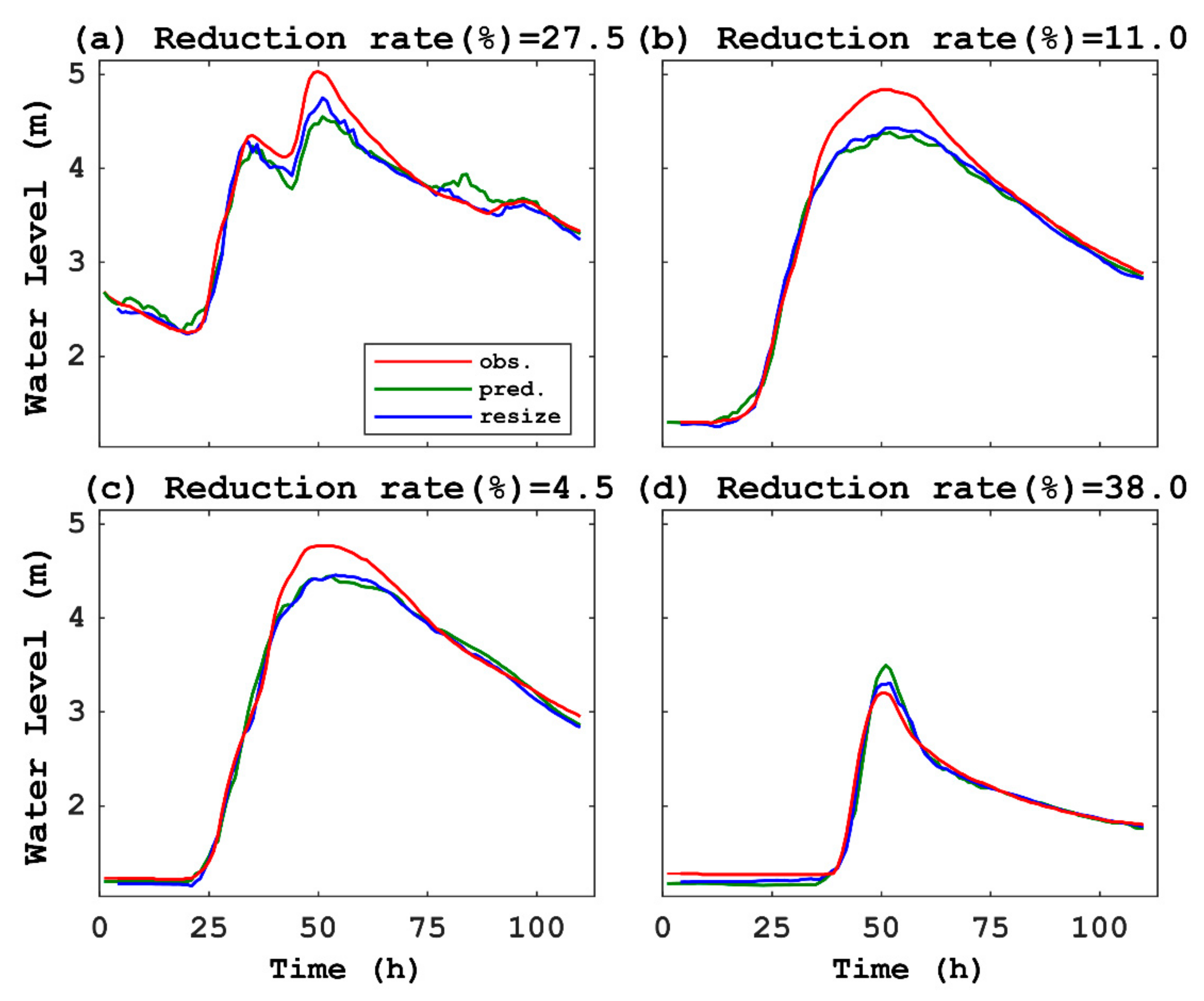
Resizing pixels in the 2D image of Domain B may affect image classification using CNN. We compared CNN predictions with an original image (123 × 13 pixels) and those with a resized image (123 × 16 pixels). Figure A2 shows water levels in four test datasets in comparison among observed data, prediction with the original image, and prediction with the resized image. The two waveforms by the CNN predictions are similar in each B1–B4. As shown in Table A2, the RMSEs between observed data and predictions in the testing of B1–B4 with the original image are from 0.19 to 0.22. In contrast, the RMSEs with the resized image are 0.06 to 0.20. The resized image caused the reduction of the RMSEs with the original image that ranges from 4.5% to 38%. This suggests that an extended image may provide better predictions on CNN time classifications possibly due to a gain of more information by larger-size pixels.
Figure A2.
Comparisons among observed data (obs.), prediction with original image (pred.), and prediction with resized image (resize) in four test datasets for water level (m) versus time (hour) in Domain B, using CNN without transfer learning: (a) highest flood event, (b) second highest flood event, (c) third highest flood event, and (d) moderate peak flood event.

Table A2.
Error evaluation of CNN between an original image and a resized image in Domain B.
| Case | RMSE (m) of CNN with an Original Image (123 × 13 Pixels): RMSEOrg | RMSE (m) of CNN with a Resized Image (123 × 16 pixels): RMSERes | Reduced Rate of RMSE (%) 1 |
|---|---|---|---|
| B1 | 0.198 | 0.144 | 27.5 |
| B2 | 0.224 | 0.200 | 11.0 |
| B3 | 0.163 | 0.155 | 4.5 |
| B4 | 0.104 | 0.064 | 38.0 |
1 Reduced rate was defined as (RMSEOrg − RMSERes)/RMSEOrg × 100.
References
- Nevo, S.; Anisimov, V.; Elidan, G.; El-Yaniv, R.; Giencke, P.; Gigi, Y.; Hassidim, A.; Moshe, Z.; Schlesinger, M.; Shalev, G.; et al. ML for Flood Forecasting at Scale. In Proceedings of the Thirty-Second Annual Conference on the Neural Information Processing Systems (NIPS), Montréal, QC, Canada, 3–8 December 2018; Available online: https://arxiv.org/pdf/1901.09583.pdf (accessed on 31 October 2019).
- Salas, F.R.; Somos-Valenzuela, M.A.; Dugger, A.; Maidment, D.R.; Gochis, D.J.; David, C.H.; Yu, W.; Ding, D.; Clark, E.P.; Noman, N. Towards real-time continental scale streamflow simulation in continuous and discrete space. J. Am. Water Resour. Assoc. JAWRA 2018, 54, 7–27. [Google Scholar] [CrossRef]
- Realestate Blog: The Worst Disasters Caused by Heavy Rain and Typhoons in Japan: 2011 to 2018. Available online: https://resources.realestate.co.jp/living/the-top-disasters-caused-by-heavy-rain-and-typhoons-in-japan-2011-to-2018/ (accessed on 31 October 2019).
- Tokar, A.S.; Markus, M. Precipitation-runoff modeling using artificial neural networks and conceptual moldes. J. Hydrol. Eng. 2000, 5, 156–161. [Google Scholar] [CrossRef]
- Akhtar, M.K.; Corzo, G.A.; van Andel, S.J.; Jonoski, A. River flow forecasting with artificial neural networks using satellite observed precipitation pre-processed with flow length and travel time information: Case study of the Ganges river basin. Hydrol. Earth Syst. Sci. 2009, 13, 1607–1618. [Google Scholar] [CrossRef] [Green Version]
- Maier, H.R.; Jain, A.; Dandy, G.C.; Sudheer, K.P. Methods used for the development of neural networks for the prediction of water resource variables in river systems: Current status and future directions. Environ. Model. Softw. 2010, 25, 891–909. [Google Scholar] [CrossRef]
- Hitokoto, M.; Sakuraba, M.; Sei, Y. Development of the real-time river stage prediction method using deep learning. J. Jpn. Soc. Civ. Eng. JSCE Ser. B1 Hydraul. Eng. 2016, 72, I_187–I_192. [Google Scholar] [CrossRef] [Green Version]
- Hochreiter, P.; Schmidhuber, J. Long short-term memory. Neural Comput. 1997, 9, 1735–1780. [Google Scholar] [CrossRef] [PubMed]
- Gers, F.A.; Schmidhuber, J.; Cummins, F. Learning to forget: Continual prediction with LSTM. In Proceedings of the 9th International Conference on Artificial Neural Networks (ICANN) 99, Edinburgh, UK, 7–10 September 1999; Volume 9, pp. 850–855. [Google Scholar] [CrossRef]
- Yamada, K.; Kobayashi, Y.; Nakatsugawa, M.; Kishigami, J. A case study of flood water level prediction in the Tokoro River in 2016 using recurrent neural networks. J. Jpn. Soc. Civ. Eng. JSCE Ser. B1 Hydraul. Engr. 2018, 74, I_1369–I_1374. (In Japanese) [Google Scholar] [CrossRef]
- Hu, C.; Wu, Q.; Li, H.; Jian, S.; Li, N.; Lou, Z. Deep learning with a long short-term memory networks approach for rainfall-runoff simulation. Water 2018, 10, 1543. [Google Scholar] [CrossRef] [Green Version]
- Le, X.; Ho, H.V.; Lee, G.; Jung, S. Application of long short-term memory (LSTM) neural network for flood forecasting. Water 2019, 11, 1387. [Google Scholar] [CrossRef] [Green Version]
- Pratt, L.Y. Discriminability-Based Transfer between Neural Networks. In Proceedings of the Conference of the Advances in NIPS 5, Denver, CO, USA, 30 November–3 December 1992; pp. 204–211. [Google Scholar]
- Laptev, N.; Yu, J.; Rajagopal, R. Reconstruction and regression loss for time-series transfer learning. In Proceedings of the Special Interest Group on Knowledge Discovery and Data Mining (SIGKDD) and the 4th Workshop on the Mining and LEarning from Time Series (MiLeTS), London, UK, 20 August 2018. [Google Scholar]
- Potikyan, N. Transfer Learning for Time Series Prediction. Available online: https://towardsdatascience.com/transfer-learning-for-time-series-prediction-4697f061f000 (accessed on 31 October 2019).
- LeCun, Y.; Bottou, L.; Bengio, Y.; Haffner, P. Gradient-based learning applied to document recognition. Proc. IEEE 1998, 86, 2278–2324. [Google Scholar] [CrossRef] [Green Version]
- Kensert, A.; Harrison, P.J.; Spjuth, O. Transfer learning with deep convolutional neural networks for classifying cellular morphological changes. SLAS Discov. 2019, 24, 466–475. [Google Scholar] [CrossRef] [PubMed] [Green Version]
- Kolar, Z.; Chen, H.; Luo, X. Transfer learning and deep convolutional neural networks for safety guardrail detection in 2D images. Autom. Constr. 2018, 89, 58–70. [Google Scholar] [CrossRef]
- Visual Geometry Group, Department of Engineering Science, University of Oxford. Available online: http://www.robots.ox.ac.uk/~vgg/research/very_deep/ (accessed on 31 October 2019).
- Nakayama, H. Image feature extraction and transfer learning using deep convolutional neural networks. Inst. Electron. Inf. Commun. Eng. IEICE Tech. Rep. 2015, 115, 55–59. Available online: https://www.ieice.org/ken/paper/20150717EbBB/eng/ (accessed on 31 October 2019).
- Zeiler, M.D.; Fergus, R. Visualizing and understanding convolutional networks. In Computer Vision—ECCV 2014; Fleet, D., Pajdla, T., Schiele, B., Tuytelaars, T., Eds.; Springer International Publishing: Cham, Switzerland, 2014; pp. 818–833. [Google Scholar]
- Miyazaki, K.; Matsuo, Y. Stock prediction analysis using deep learning technique. In Proceedings of the 31st Annual Conference of the Japanese Society for Artificial Intelligence, Nagoya, Japan, 23–26 May 2017. (In Japanese). [Google Scholar]
- Suzuki, T.; Kim, S.; Tachikawa, Y.; Ichikawa, Y.; Yorozu, K. Application of convolutional neural network to occurrence prediction of heavy rainfall. J. Jpn. Soc. Civ. Eng. JSCE Ser. B1 Hydraul. Engr. 2018, 74, I_295–I_300. (In Japanese) [Google Scholar] [CrossRef]
- Ministry of Land, Infrastructure, Transport, and Tourism in Japan (MLIT Japan). Hydrology and Water Quality Database. Available online: http://www1.river.go.jp/ (accessed on 31 October 2019).
- Japan Meteorological Agency (JMA). Past Meteorological Data. Available online: http://www.data.jma.go.jp/gmd/risk/obsdl/index.php (accessed on 31 October 2019).
- Lanczos, C. An iteration method for the solution of the eigenvalue problem of linear differential and integral operators. J. Res. National Bur. Stand. 1950, 45, 255–282. [Google Scholar] [CrossRef]
- James, G.; Witten, D.; Hastie, T.; Tibshirani, R. An Introduction to Statistical Learning: With Applications in R, 1st ed.; Springer: New York, NY, USA, 2013; p. 176. ISBN 978-1461471370. [Google Scholar]
- Brownlee, J. Blog: What Is the Difference between Test and Validation Datasets? Available online: https://machinelearningmastery.com/difference-test-validation-datasets/ (accessed on 31 October 2019).
- Python. Available online: http://www.python.org (accessed on 31 October 2019).
- Keras: The Python Deep Learning Library. Available online: https://keras.io/ (accessed on 31 October 2019).
- Rumelhart, D.E.; EHinton, G.E.; Williams, R.J. Learning representations by back-propagating errors. Nature 1986, 323, 533–536. [Google Scholar] [CrossRef]
- Lachenbruch, P.A.; Mickey, M.R. Estimation of error rates in discriminant analysis. Technometrics 1968, 10, 1–11. [Google Scholar] [CrossRef]
- Mosavi, A.; Ozturk, P.; Chau, K. Flood prediction using machine learning models: Literature review. Water 2018, 10, 1536. [Google Scholar] [CrossRef] [Green Version]
- Wang, S.H.; Xie, S.; Chen, X.; Guttery, D.S.; Tang, C.; Sun, J.; Zhang, Y. Alcoholism identification based on an AlexNet transfer learning model. Front. Psychiatry 2019, 10, 205. [Google Scholar] [CrossRef] [PubMed] [Green Version]
Figure 1.
Maps of field sites: Domain A is part of the Oyodo River watershed, and Domain B is the Abashiri River watershed.
Figure 1.
Maps of field sites: Domain A is part of the Oyodo River watershed, and Domain B is the Abashiri River watershed.

Figure 2.
Structures of artificial neural network (ANN) model that show (a) data flows in the ANN with deep learning (○ = neuron) and (b) the inner structure of a neuron of jth with i-1th, ith, and i+1th inputs with weighed coefficients.
Figure 2.
Structures of artificial neural network (ANN) model that show (a) data flows in the ANN with deep learning (○ = neuron) and (b) the inner structure of a neuron of jth with i-1th, ith, and i+1th inputs with weighed coefficients.

Figure 3.
Depiction of the convolution layer with a filter in convolutional neural network (CNN).

Figure 4.
Simple overviews that show the model predictions with transfer learning (right) or without (left) transfer learning in Domains A and Domain B. The transfer learning extracts the features as common knowledge from Domain A and then applies common knowledge to predict in model B.
Figure 4.
Simple overviews that show the model predictions with transfer learning (right) or without (left) transfer learning in Domains A and Domain B. The transfer learning extracts the features as common knowledge from Domain A and then applies common knowledge to predict in model B.

Figure 5.
Data flows in procedures (a) CNN and (b) CNN with transfer learning.

Figure 6.
Sample data conversion from time-series data to image data.

Figure 7.
Sketch that shows the creation of a dataset from a 2D image to one value at the predicted point.
Figure 7.
Sketch that shows the creation of a dataset from a 2D image to one value at the predicted point.

Figure 8.
Comparisons between observed data (obs.) and prediction (pred.) in four test datasets of water level (m) versus time (hour) in domain: (a) third highest flood event, (b) second highest flood event, (c) highest flood event, and (d) moderate peak flood event.
Figure 8.
Comparisons between observed data (obs.) and prediction (pred.) in four test datasets of water level (m) versus time (hour) in domain: (a) third highest flood event, (b) second highest flood event, (c) highest flood event, and (d) moderate peak flood event.

Figure 9.
Error evaluation of the number of retrainings using CNN transfer learning.

Figure 10.
Comparisons between observed data (obs.) and prediction (pred.) in four test datasets for water level (m) versus time (hour) in Domain B, using CNN transfer learning with 20-time retrainings: (a) highest flood event, (b) second highest flood event, (c) third highest flood event, and (d) moderate peak flood event.

Table 1.
Flood events in Domain A.
| Event Name | Start Time 1 | End Time 1 | Maximum Water Level (m) During Each Event 2,3 | Remarks |
|---|---|---|---|---|
| 8/5/1992 | 8/5/1992 21:00 | 8/10/1992 23:00 | 4.56 | |
| 7/29/1993 | 7/29/1993 20:00 | 8/3/1993 22:00 | 9.50 | 3rd position |
| 8/7/1993 | 8/7/1993 2:00 | 8/12/1993 4:00 | 8.04 | |
| 8/13/1993 | 8/31/1993 19:00 | 9/5/1993 21:00 | 6.99 | |
| 6/10/1994 | 6/10/1994 20:00 | 6/15/1994 22:00 | 4.80 | |
| 6/1/1995 | 6/1/1995 6:00 | 6/6/1995 8:00 | 4.66 | |
| 6/22/1995 | 6/22/1995 15:00 | 6/27/1995 17:00 | 6.90 | |
| 7/15/1996 | 7/15/1996 19:00 | 7/20/1996 21:00 | 6.84 | |
| 8/11/1996 | 8/11/1996 23:00 | 8/17/1996 1:00 | 5.18 | |
| 8/4/1997 | 8/4/1997 0:00 | 8/9/1997 2:00 | 5.05 | |
| 7/24/1999 | 7/24/1999 0:00 | 7/29/1999 2:00 | 6.72 | |
| 8/14/1999 | 8/14/1999 15:00 | 8/19/1999 17:00 | 6.03 | |
| 9/11/1999 | 9/11/1999 20:00 | 9/16/1999 22:00 | 8.26 | |
| 9/21/1999 | 9/21/1999 19:00 | 9/26/1999 21:00 | 5.42 | |
| 5/31/2000 | 5/31/2000 14:00 | 6/5/2000 16:00 | 6.47 | |
| 6/18/2001 | 6/18/2001 20:00 | 6/23/2001 22:00 | 5.30 | |
| 8/5/2003 | 8/5/2003 10:00 | 8/10/2003 12:00 | 6.79 | |
| 8/27/2004 | 8/27/2004 10:00 | 9/1/2004 12:00 | 9.80 | 2nd position |
| 10/17/2004 | 10/17/2004 9:00 | 10/22/2004 11:00 | 7.70 | |
| 9/3/2005 | 9/3/2005 8:00 | 9/8/2005 10:00 | 10.65 | highest peak |
| 6/21/2006 | 6/21/2006 23:00 | 6/27/2006 1:00 | 4.99 | |
| 7/19/2006 | 7/19/2006 11:00 | 7/24/2006 13:00 | 5.28 | |
| 8/15/2006 | 8/15/2006 18:00 | 8/20/2006 20:00 | 5.20 | |
| 7/8/2007 | 7/8/2007 21:00 | 7/13/2007 23:00 | 5.58 | |
| 7/11/2007 | 7/11/2007 15:00 | 7/16/2007 17:00 | 7.11 | |
| 9/28/2008 | 9/28/2008 16:00 | 10/3/2008 18:00 | 5.18 | |
| 6/17/2010 | 6/17/2010 18:00 | 6/22/2010 20:00 | 6.30 | |
| 6/30/2010 | 6/30/2010 7:00 | 7/5/2010 9:00 | 9.16 | |
| 6/13/2011 | 6/13/2011 23:00 | 6/19/2011 1:00 | 4.84 | |
| 6/18/2011 | 6/18/2011 0:00 | 6/23/2011 2:00 | 4.77 | |
| 6/19/2012 | 6/19/2012 7:00 | 6/24/2012 9:00 | 5.13 | |
| 6/25/2012 | 6/25/2012 7:00 | 6/30/2012 9:00 | 4.60 | |
| 7/10/2012 | 7/10/2012 18:00 | 7/15/2012 20:00 | 5.86 | |
| 6/25/2014 | 6/25/2014 10:00 | 6/30/2014 12:00 | 5.31 | |
| 7/28/2014 | 7/28/2014 17:00 | 8/2/2014 19:00 | 6.61 | |
| 8/6/2014 | 8/6/2014 8:00 | 8/11/2014 10:00 | 6.08 | |
| 7/19/2015 | 7/19/2015 18:00 | 7/24/2015 20;00 | 5.05 | |
| 8/22/2015 | 8/22/2015 18:00 | 8/27/2015 20:00 | 4.62 | |
| 6/25/2016 | 6/25/2016 19:00 | 6/30/2016 21:00 | 6.09 | |
| 7/6/2016 | 7/6/2016 3:00 | 7/11/2016 5:00 | 5.52 | |
| 7/11/2016 | 7/11/2016 11:00 | 7/16/2016 13:00 | 6.21 | |
| 9/17/2016 | 9/17/2016 5:00 | 9/22/2016 7:00 | 7.91 | |
| 8/4/2017 | 8/4/2017 5:00 | 8/9/2017 7:00 | 5.13 |
1 Date and time is denoted as month/day/year hour:minute; 2 Maximum value at each event was observed at Hiwatashi Station; 3 Risk levels for near flooding occurrence and flooding cautionary exceed 9.20 and 6.00 m, respectively.
Table 2.
Flood events in Domain B.
| Event Name | Start Time 1 | End Time 1 | Maximum Water Level (m) During Each Event 2,3 | Remarks |
|---|---|---|---|---|
| 4/9/2000 | 4/9/2000 8:00 | 4/14/2000 10:00 | 3.81 | |
| 9/9/2001 | 9/9/2001 18:00 | 9/14/2001 20:00 | 4.84 | 2nd position |
| 9/30/2002 | 9/30/2002 2:00 | 10/5/2002 4:00 | 3.38 | |
| 8/7/2003 | 8/7/2003 21:00 | 8/12/2003 23:00 | 4.28 | |
| 4/18/2006 | 4/18/2006 22:00 | 4/24/2006 0:00 | 3.30 | |
| 8/17/2006 | 8/17/2006 1:00 | 8/22/2006 3:00 | 4.04 | |
| 10/6/2006 | 10/6/2006 2:00 | 10/11/2006 4:00 | 4.77 | 3rd position |
| 10/7/2009 | 10/7/2009 5:00 | 10/12/2009 7:00 | 3.33 | |
| 9/20/2011 | 9/20/2011 0:00 | 9/25/2011 2:00 | 3.20 | |
| 4/5/2013 | 4/5/2013 7:00 | 4/10/2013 9:00 | 3.71 | |
| 9/14/2013 | 9/14/2013 13:00 | 9/19/2013 15:00 | 4.33 | |
| 10/6/2015 | 10/6/2015 9:00 | 10/11/2015 11:00 | 4.15 | |
| 8/15/2016 | 8/15/2016 16:00 | 8/20/2016 18:00 | 4.17 | |
| 8/19/2016 | 8/19/2016 4:00 | 8/24/2016 6:00 | 5.03 | highest peak |
| 8/28/2016 | 8/28/2016 21:00 | 9/2/2016 23:00 | 3.46 | |
| 9/7/2016 | 9/7/2016 12:00 | 9/12/2016 14:00 | 4.15 | |
| 8/7/2019 | 8/7/2019 0:00 | 8/12/2019 2:00 | 3.22 | provisional value |
1 Date and time is denoted as month/day/year hour:minute. 2 Maximum value at each event was observed at Hongou Station. 3 Risk levels for near flooding occurrence and flooding cautionary exceed 5.30 and 3.20 m, respectively.
Table 3.
Characteristics of the two domains.
| Domain A | Domain B | |
|---|---|---|
| Number of events | 43 | 17 |
| Maximum water level (at prediction location) | 10.65 m | 5.03 m |
| Number of water level stations | 5 | 4 |
| Number of rainfall stations | 11 | 9 |
| Watershed area | 861 km2 | 1319 km2 |
| Prediction location | Hiwatashi (31.8599° N, 131.1135° E) | Hongou (43.9096° N, 144.1385° E) |
| Main river name | Oyodo River | Abashiri River |
Table 4.
Source datasets for training, validation, and testing in Domain A.
| Source Case | Training Datasets | Validation Datasets | Test Dataset |
|---|---|---|---|
| A1 | 8/5/1992, 8/31/1993, 6/10/1994, 6/1/1995, 6/22/1995, 7/15/1996, 8/11/1996, 8/4/1997, 7/24/1999, 9/11/1999, 9/21/1999, 5/31/2000, 5/31/2000, 6/18/2001, 8/5/2003, 10/17/2004, 6/21/2006, 7/19/2006, 8/15/2006, 7/8/2007, 7/11/2007, 9/28/2008, 6/17/2010, 6/30/2010, 6/13/2011, 6/19/2012, 6/25/2012, 7/10/2012, 6/25/2014, 7/28/2014, 8/6/2014, 7/19/2015, 8/22/2015, 6/25/2016, 7/6/2016, 7/11/2016, 9/17/2016, 8/4/2017 | 8/7/1993, 8/14/1999, 8/27/2004, 9/3/2005 | 7/29/1993 |
| A2 | 7/29/1993, 8/7/1993, 8/14/1999, 9/3/2005 | 8/27/2004 | |
| A3 | 7/29/1993, 8/7/1993, 8/14/1999, 8/27/2004 | 9/3/2005 | |
| A4 | 7/29/1993, 8/7/1993, 8/27/2004, 9/3/2005 | 8/14/1999 |
Table 5.
Target datasets for training, validation, and testing in Domain B.
| Source Case | Training Datasets | Verification Datasets | Test Dataset |
|---|---|---|---|
| B1 | 9/30/2002, 8/7/2003, 4/18/2006, 8/17/2006, 10/7/2009, 4/5/2013, 9/14/2013, 10/6/2015, 8/15/2016, 8/28/2016, 9/7/2016, 8/7/2019 | 4/9/2000, 9/9/2001, 10/6/2006, 9/20/2011 | 8/19/2016 |
| B2 | 4/9/2000, 10/6/2006, 9/20/2011, 8/19/2016 | 9/9/2001 | |
| B3 | 4/9/2000, 9/9/2001, 9/20/2011, 8/19/2016 | 10/6/2006 | |
| B4 | 4/9/2000, 9/9/2001, 10/6/2006, 8/19/2016 | 9/20/2011 |
Table 6.
Setups of CNN parameters and functions.
| Parameters | Values/Function | Remarks | |
|---|---|---|---|
| Convolutional layer | Filter size | 3 × 3 | |
| Filter number | 5 | ||
| Pooling layer | Filter size | 2 × 2 | |
| Fully connected layer 1 | Neuron number | 16 | |
| Fully connected layer 2 | Neuron number | 1 | |
| Learning process | Batch size | 100 | |
| Epoch number | 100 | ||
| Learning rate | 0.001 | ||
| Optimizer | Adam | ||
| Activation function 1 to 3 | ReLU | See Figure 5a | |
| Activation function 4 | Sigmoid/softmax | See Figure 5a | |
| Loss function | Mean square error = | ci = model prediction, oi = observed data, N1 = the number of data | |
| Error evaluation | Root mean square error (RMSE) = | Same as above | |
Table 7.
Error evaluation of the CNN in Domain A.
| Case | RMSE (m) | Relative Error (%) 1 |
|---|---|---|
| A1 | 0.464 | 6.45 |
| A2 | 0.370 | 3.79 |
| A3 | 0.734 | 6.93 |
| A4 | 0.136 | 2.58 |
1 Relative error was the RMSE divided by the variation between minimum water level and maximum water level in each test dataset.
Table 8.
Error evaluation of the CNN transfer learning with 20-time retrainings in Domain B.
| Case | RMSE (m) | Relative Error (%) 1 | Reference: RMSE (m) of CNN Without Transfer Learning and With Resized Image |
|---|---|---|---|
| B1 | 0.118 | 4.24 | 0.144 |
| B2 | 0.153 | 4.30 | 0.200 |
| B3 | 0.125 | 3.52 | 0.155 |
| B4 | 0.064 | 3.34 | 0.064 |
1 Relative error was the same as that in Table 7.
© 2019 by the authors. Licensee MDPI, Basel, Switzerland. This article is an open access article distributed under the terms and conditions of the Creative Commons Attribution (CC BY) license (http://creativecommons.org/licenses/by/4.0/).
Share and Cite
MDPI and ACS Style
Kimura, N.; Yoshinaga, I.; Sekijima, K.; Azechi, I.; Baba, D. Convolutional Neural Network Coupled with a Transfer-Learning Approach for Time-Series Flood Predictions. Water 2020, 12, 96. https://doi.org/10.3390/w12010096
AMA Style
Kimura N, Yoshinaga I, Sekijima K, Azechi I, Baba D. Convolutional Neural Network Coupled with a Transfer-Learning Approach for Time-Series Flood Predictions. Water. 2020; 12(1):96. https://doi.org/10.3390/w12010096
Chicago/Turabian StyleKimura, Nobuaki, Ikuo Yoshinaga, Kenji Sekijima, Issaku Azechi, and Daichi Baba. 2020. "Convolutional Neural Network Coupled with a Transfer-Learning Approach for Time-Series Flood Predictions" Water 12, no. 1: 96. https://doi.org/10.3390/w12010096
Note that from the first issue of 2016, this journal uses article numbers instead of page numbers. See further details here.