Modeling the Ecological Response of a Temporarily Summer-Stratified Lake to Extreme Heatwaves

 ,
,  , and
, and
Abstract
:
1. Introduction
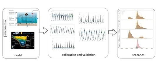
2. Methods
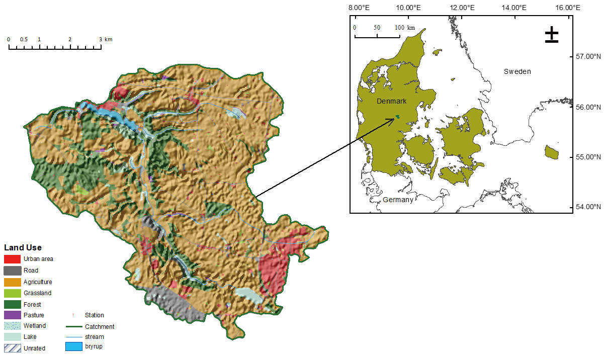
2.1. Study Site
2.2. Model Description
2.3. Model Input Data
2.4. Model Calibration and Validation
2.5. Base Scenario and Extreme Climate Scenarios
3. Results
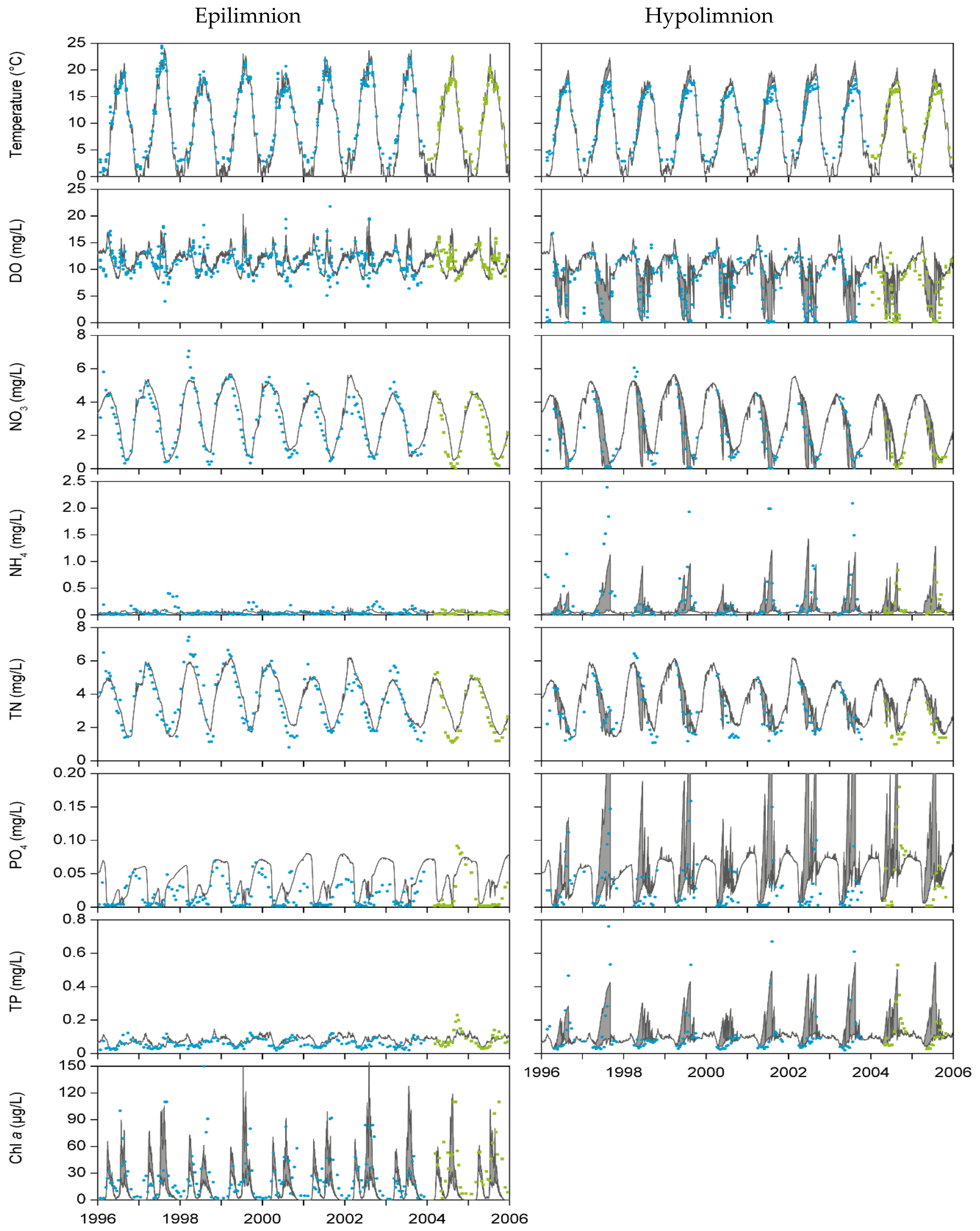
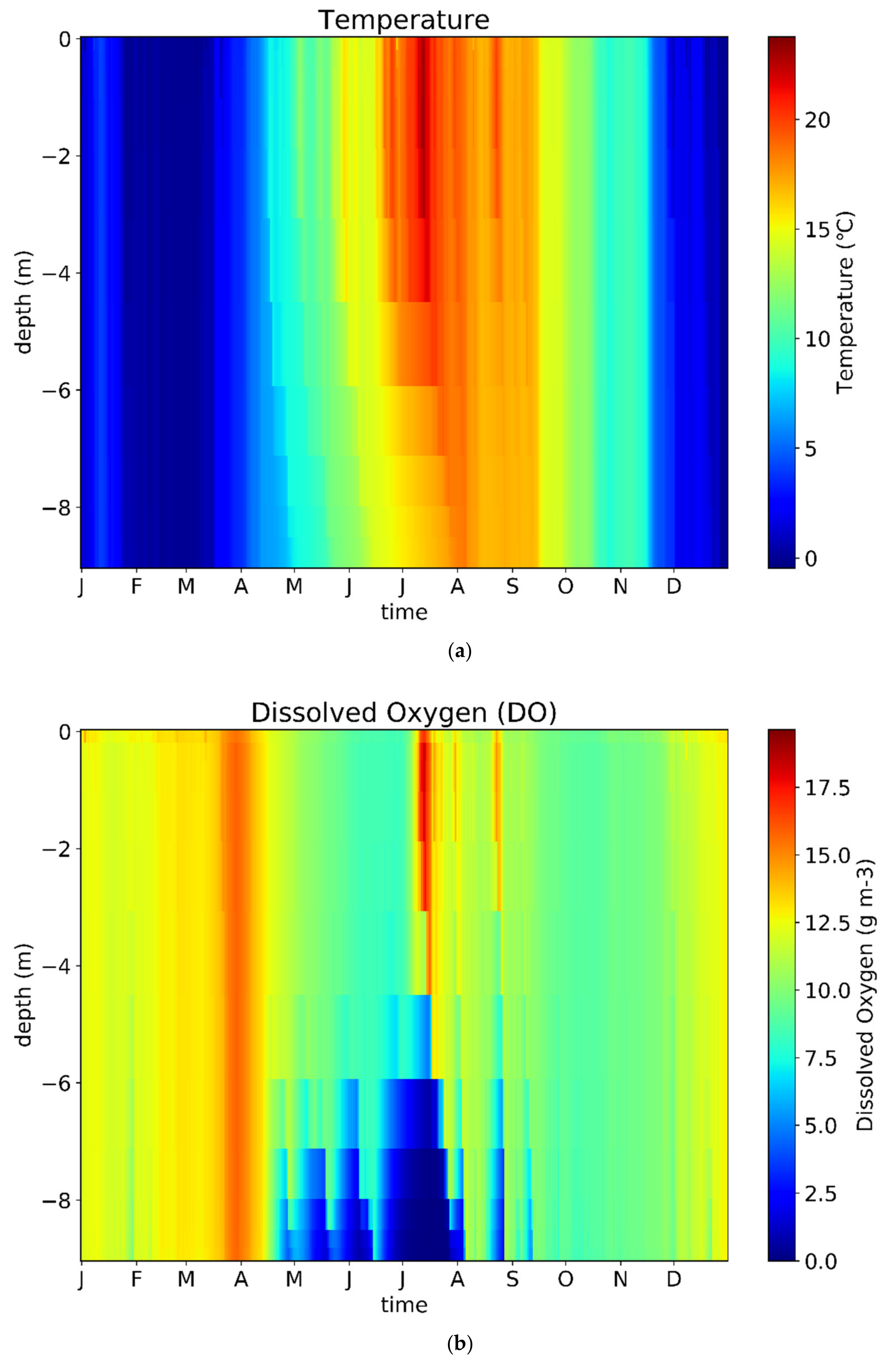
3.1. Model Calibration and Validation
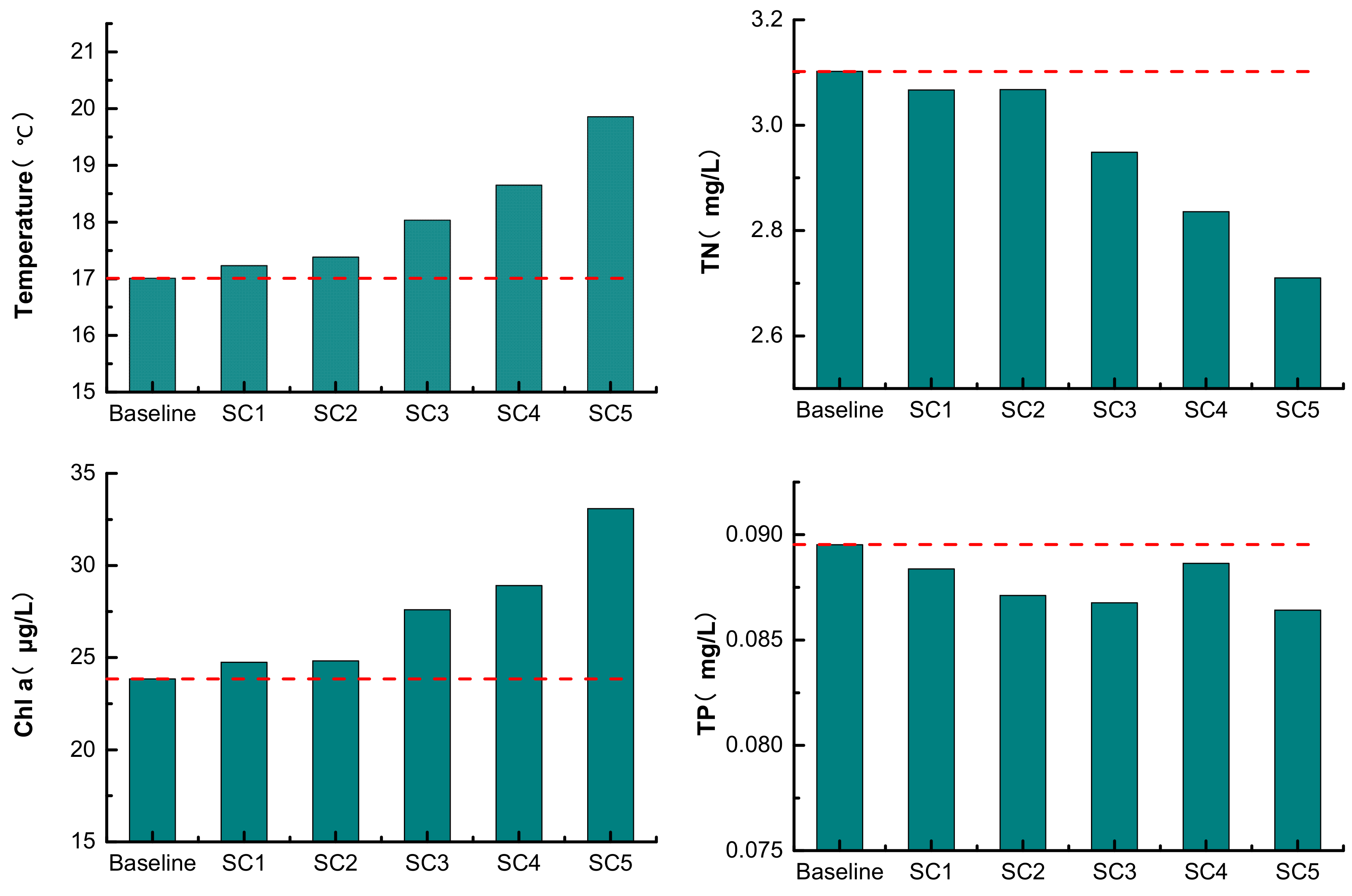
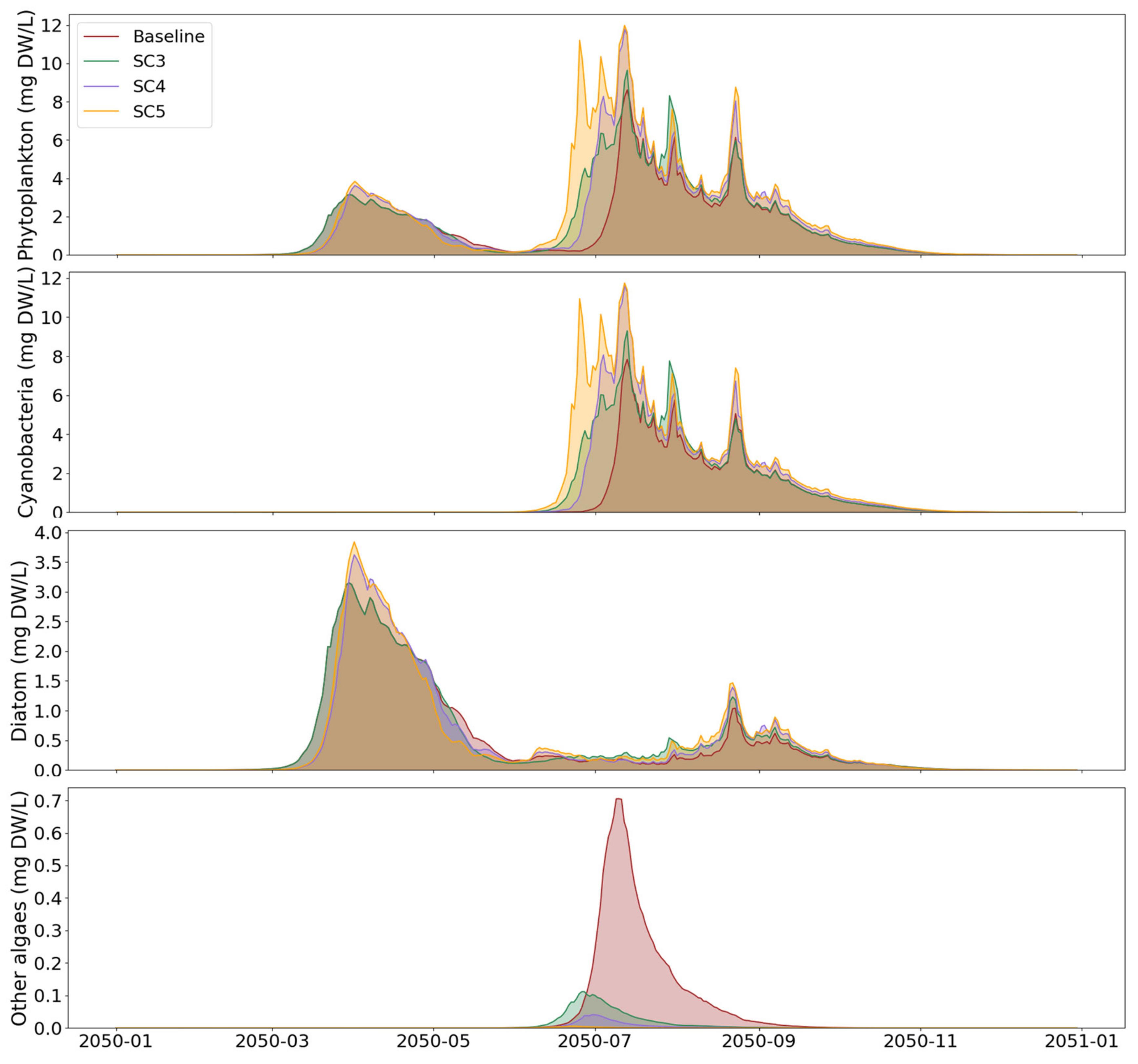
3.2. Extreme Climate Scenarios
4. Discussion
4.1. Model Performance
4.2. Effects of Extreme Temperatures
4.3. Study Constraints
4.4. Implications for Lake Management
Author Contributions
Funding
Acknowledgments
Conflicts of Interest
Appendix A
| Parameter | Description | Unit | Parameter Value | |
| Default | Adjusted | |||
| Abiotic_Water Module | ||||
| cThetaAer | temperature coefficient for reaeration | [−] | 1.024 | 1.005 |
| cThetaNitr | temperature coefficient for nitrification | [−] | 1.08 | 1.003 |
| cVSetPOM | maximum settling rate of POM | m·day−1 | −0.25 | −0.35 |
| cVSetIM | maximum settling rate of inorganic matter | m·day−1 | −1.0 | −0.95 |
| hNO3Denit | quadratic half saturation NO3 conc. for denitrification | mgN·L−1 | 2.0 | 0.3 |
| hO2BOD | half saturation oxygen conc. for BOD | mgO2·L−1 | 1.0 | 4.79 |
| hO2Nitr | half saturation oxygen conc. for nitrification | mgO2·L−1 | 2.0 | 3.57 |
| kNitrW | nitrification rate constant in water | day−1 | 0.1 | 0.39 |
| NO3PerC | denitrified NO3 per mol C mineralised | mol NO3 | 0.8 | 1.47 |
| O2PerNH4 | used O2 per mol NH4+ nitrified | mol O2 | 2.0 | 3.30 |
| cThetaMinPOMW | temperature coefficient for mineralization from POM to DOM | [−] | 1.07 | 1.01 |
| kDMinPOMW | decomposition constant for POM-DW to DOM-DW | day−1 | 0.01 | 0.0001 |
| kNMinPOMW | decomposition constant for POM-N to DOM-N | day−1 | 0.01 | 0.014 |
| kPMinPOMW | decomposition constant for POM-P to DOM-P | day−1 | 0.01 | 0.0003 |
| kSiMinPOMW | decomposition constant for POM-Si to DOM-Si | day−1 | 0.01 | 0.0097 |
| cThetaMinDOMW | temperature coefficient for DOM mineralization | [−] | 1.07 | 1.05 |
| kDMinDOMW | mineralization constant of dissolved organic DW | day−1 | 0.01 | 0.035 |
| kNMinDOMW | mineralization constant of dissolved organic N | day−1 | 0.01 | 0.016 |
| kPMinDOMW | mineralization constant of dissolved organic P | day−1 | 0.01 | 0.014 |
| kSiMinDOMW | mineralization constant of dissolved organic Si | day−1 | 0.01 | 0.0083 |
| Abiotic_Sediment Module | ||||
| fRefrPOMS | refractory fraction of sediment POM | [−] | 0.15 | 0.08 |
| O2PerNH4 | O2 used per mol NH4+ nitrified | mol | 2.0 | 1.71 |
| kNitrS | nitrification rate constant | day−1 | 1.0 | 0.34 |
| cThetaNitr | temperature coefficient for nitrification | [−] | 1.08 | 1.01 |
| NO3PerC | NO3 denitrified per mol C mineralised | [−] | 0.8 | 0.91 |
| hNO3Denit | quadratic half-sat. NO3 conc. for denitrification | mgN·L−1 | 2.0 | 0.25 |
| kPSorp | P sorption rate constant not too high -> model speed | day−1 | 0.05 | 0.089 |
| cRelPAdsD | max. P adsorption per g DW | gP·gD−1 | 3 × 10⁻⁵ | 4.76 × 10⁻⁵ |
| cRelPAdsFe | max. P adsorption per g Fe | gP·gFe−1 | 0.065 | 0.055 |
| fFeDIM | Fe content of inorganic. matter | gFe·Gd−1 | 0.01 | 0.026 |
| fRedMax | max. reduction factor of P adsorption affinity | [−] | 0.9 | 0.86 |
| cKPAdsOx | P adsorption affinity at oxidized conditions | m3·gP−1 | 0.6 | 1.6 |
| coPO4Max | max. SRP conc. in pore water | mgP·L−1 | 1.0 | 1.04 |
| cThetaDif | temperature coefficient for diffusion | [−] | 1.02 | 1.02 |
| kNDifNH4 | molecular NH4 diffusion constant | m2·day−1 | 0.000112 | 0.000112 |
| cTurbDifNut | bioturbation factor for diffusion | [−] | 5.0 | 14.76 |
| kO2Dif | molecular O2 diffusion constant | m2·day−1 | 2.6 × 10⁻⁵ | 0.00018 |
| cTurbDifO2 | bioturbation factor for diffusion | [−] | 5.0 | 1.93 |
| kDMinHum | maximum decomposition constant of humic material (1D−5) | day−1 | 1 × 10⁻⁵ | 0.00021 |
| cThetaMinPOMS | temperature coeff. for sediment mineralization of POM to DOM | [−] | 1.07 | 1.05 |
| kDMinPOMS | mineralization constant in sediment from POM-DW to DOM-DW | day−1 | 0.002 | 0.0027 |
| kNMinPOMS | mineralization constant in sediment from POM-N to DOM-N | day−1 | 0.002 | 0.0002 |
| kPMinPOMS | mineralization constant in sediment from POM-P to DOM-P | day−1 | 0.002 | 0.0001 |
| cThetaMinDOMS | exp. temperature constant of sediment mineralization | [−] | 1.07 | 1.02 |
| kDMinDOMS | mineralization constant for sediment dissolved organic matter | day−1 | 0.002 | 0.0027 |
| kNMinDOMS | mineralization constant for sediment dissolved organic N | day−1 | 0.002 | 0.0017 |
| kPMinDOMS | mineralization constant for sediment dissolved organic P | day−1 | 0.002 | 0.0022 |
| kSiMinDOMS | mineralization constant for sediment dissolved organic Si | day−1 | 0.002 | 0.0019 |
| kDDifDOM | molecular diffusion constant for dissolved organic matter | m2·day−1 | 0.000112 | 0.0029 |
| kNDifDOM | molecular diffusion constant for dissolved organic N | m2·day−1 | 0.000112 | 0.000118 |
| kPDifDOM | molecular diffusion constant for dissolved organic P | m2·day−1 | 0.000112 | 0.000118 |
| sPAIMS | sediment absorbed phosphate | g·m−2 | 2.0 | 0.5 |
| sDPOMS | sediment particulate organic DW | g·m−2 | 474 | 1104 |
| sNPOMS | sediment particulate organic N | g·m−2 | 6.0 | 15.13 |
| sPPOMS | sediment particulate organic | g·m−2 | 1.0 | 10 |
| sDHumS | sediment humus DW | g·m−2 | 3719 | 4488 |
| Phytoplankton_Water Module | ||||
| cSigTmDiat | temperature constant diatoms (sigma in Gaussian curve) | °C | 20.0 | 15.66 |
| cTmOptDiat | optimum temperature of diatoms | °C | 18.0 | 20.29 |
| cSigTmBlue | temperature constant blue-greens (sigma in Gaussian curve) | °C | 12.0 | 12.16 |
| cTmOptBlue | optimum temperature of blue-greens | °C | 25.0 | 28.11 |
| cSigTmGren | temperature constant greens (sigma in Gaussian curve) | °C | 15.0 | 12.12 |
| cTmOptGren | optimum temperature of greens | °C | 25.0 | 19.09 |
| cPDDiatMin | minimum P/DW ratio for diatoms | mg P·mg DW−1 | 0.0005 | 0.0024 |
| cNDDiatMin | minimum N/DW ratio for diatoms | mg N·mg DW−1 | 0.01 | 0.005 |
| cPDGrenMin | minimum P/DW ratio greens | mg P·mg DW−1 | 0.0015 | 0.0018 |
| cNDGrenMin | minimum N/DW ratio greens | mg N·mg DW−1 | 0.02 | 0.013 |
| cPDBlueMin | minimum P/DW ratio blue-greens | mg P·mg DW−1 | 0.0025 | 0.0012 |
| cNDBlueMin | minimum N/DW ratio blue-greens | mg N·mg DW−1 | 0.03 | 0.018 |
| cLOptRefDiat | optimum PAR for diatoms at 20 °C | W·m−2 | 54.0 | 23.32 |
| cLOptRefGren | optimum PAR for greens at 20 °C | W·m−2 | 30.0 | 35.82 |
| cLOptRefBlue | optimum PAR for blue-greens at 20 °C | W·m−2 | 13.6 | 13 |
| cMuMaxBlue | maximum growth rate blue-greens | day−1 | 0.6 | 1.38 |
| cMuMaxGren | maximum growth rate greens | day−1 | 1.5 | 1.13 |
| cMuMaxDiat | maximum growth rate diatoms | day−1 | 2.0 | 3 |
| kMortBlueW | mortality constant of blue-greens in water | day−1 | 0.01 | 0.15 |
| cVNUptMaxDiat | maximum N uptake capacity of diatoms | mg N·mg DW−1·day−1 | 0.07 | 0.067 |
| cVNUptMaxBlue | maximum N uptake capacity of blue-greens | mg N·mg DW−1·day−1 | 0.07 | 0.079 |
| cAffNUptDiat | initial N uptake affinity diatoms | mg DW−1·day−1 | 0.2 | 0.19 |
| cAffNUptBlue | initial N uptake affinity bluegreens | mg DW−1·day−1 | 0.2 | 0.15 |
| fDissMortPhyt | soluble nutrient fraction of died algae | [−] | 0.2 | 0.41 |
| cVSetDiat | settling rate of diatoms | m day−1 | −0.5 | −0.1 |
| cVSetGren | settling rate of greens | m day−1 | −0.2 | −0.42 |
| cVSetBlue | settling rate of blue-greens | m·day−1 | 0.06 | 0.03 |
| cChDBlueMax | maximum chlorophyll/C ratio for blue-greens | mg Chl a·mg DW−1 | 0.015 | 0.0031 |
| cChDBlueMin | minimum chlorophyll/C ratio for blue-greens | mg Chl a·mg DW−1 | 0.005 | 0.014 |
| cChDDiatMax | maximum chlorophyll/C ratio for diatoms | mg Chl a·mg DW−1 | 0.012 | 0.021 |
| cChDDiatMin | minimum chlorophyll/C ratio for diatoms | mg Chl a·mg DW−1 | 0.004 | 0.010 |
| cChDGrenMax | maximum chlorophyll/C ratio for greens | mg Chl a·mg DW−1 | 0.02 | 0.020 |
| cChDGrenMin | minimum chlorophyll/C ratio for greens | mg Chl a·mg DW−1 | 0.01 | 0.0075 |
| fPrimDOMW | fraction of dissolved organic matter from water column phytoplankton | [−] | 0.5 | 0.02 |
| kDRespBlue | maintenance respiration constant blue-greens | day−1 | 0.03 | 0.047 |
| Phytoplankton_Sediment Module | ||||
| fDissMortPhyt | soluble nutrient fraction of died algae | [−] | 0.2 | 0.01 |
| Macrophytes Module | ||||
| cDVegIn | external macrophytes density | g D·m2 | 1.0 | 0.46 |
| kMigrVeg | macrophyte migration rate | day−1 | 0.001 | 0.0016 |
| cMuMaxVeg | maximum growth rate of macrophytes at 20 degrees | day−1 | 0.2 | 0.031 |
| cDCarrVeg | maximum macrophytes standing crop | g DW·m−2 | 400.0 | 207.78 |
| cDayWinVeg | day of the year for the end of growing season | day of the year | 259.0 | 218.90 |
| cTmInitVeg | temperature for onset of initial growth | °C | 9.0 | 10.08 |
| cCovSpVeg | specific cover | Gdw−1·m−2 | 0.5 | 0.27 |
| hLRefVeg | half-saturation for influence of light on macrophytes | W·m−2 PAR | 17.0 | 18.05 |
| fWinVeg | fraction surviving in winter ([−]), default = 0.3 | [−] | 0.3 | 0.31 |
| fSedUptVegMax | maximum sediment fraction of nutrient uptake | [−] | 0.998 | 0.64 |
| cHeightVeg | macrophytes height | m | 1.0 | 0.95 |
| cExtSpVeg | specific extinction of macrophytes | m2·g DW | 0.01 | 0.0043 |
| cDVegMin | minimum dry weight of macrophytes in system | g DW·m−2 | 1 × 10⁻⁵ | 5.2 × 10⁻⁵ |
| cQ10ProdVeg | temperature quotient of production | [−] | 1.2 | 1.18 |
| cQ10RespVeg | temperature quotient of respiration | [−] | 2.0 | 1.98 |
| Zooplankton Module | ||||
| cTmOptZoo | optimum temperature for zooplankton | °C | 25.0 | 17.91 |
| kDRespZoo | maintenance respiration constant for zooplankton | day−1 | 0.15 | 0.02 |
| cPrefDiat | selection factor for diatoms | [−] | 0.75 | 0.90 |
| cPrefBlue | selection factor for blue-greens | [−] | 0.125 | 0.25 |
| cPrefPOM | selection factor for particulate organic matter | [−] | 0.25 | 0.16 |
| hFilt | half-saturation constant for food conc. on zooplankton | g DW·m−3 | 1.0 | 1.19 |
| fDAssZoo | dry weight assimilation efficiency of zooplankton | [−] | 0.35 | 0.33 |
| cFiltMax | maximum filtering rate | ltr·mg DW−1·day−1 | 4.5 | 1.11 |
| fZooDOMW | dissolved organic fraction from zooplankton | [−] | 0.5 | 0.36 |
| Fish Module | ||||
| kDAssFiJv | maximum assimilation rate of zooplanktivorous fish | day−1 | 0.12 | 0.121 |
| cDCarrPiscMax | maximum carrying capacity of piscivorous fish | g DW·m−2 | 1.2 | 2.74 |
| cCovVegMin | minimum submerged macrophytes coverage for piscivorous fish | % | 40.0 | 25.67 |
| hDVegPisc | half-saturation constant for macrophytes on piscivorous fish | g·m−2 | 5.0 | 2.08 |
| Zoobenthos Module | ||||
| fBenDOMS | dissolved organic fraction from zoobenthos | [−] | 0.5 | 0.52 |
| Auxiliary Module | ||||
| kVegResus | relative resuspension reduction per gram macrophytes | m2·g DW−1 | 0.01 | 0.05 |
| kTurbFish | relative resuspension by adult fish browsing | g·gfish−1·day−1 | 1.0 | 2.15 |
| cVSedPOM | maximum sedimentation velocity of POM | m·day−1 | 0.25 | 0.5 |
| cVSedDiat | sedimentation velocity of diatoms | m·day−1 | 0.5 | 0.68 |
| cVSedGren | sedimentation velocity of greens | m·day−1 | 0.2 | 0.54 |
| cVSedBlue | sedimentation velocity of blue-greens | m·day−1 | 0.06 | 0.01 |
| crt_shear | critical shear stress | N·m−2 | 0.005 | 0.014 |
References
- Griggs, D.J.; Noguer, M. Climate change 2001: The scientific basis. Contribution of Working Group I to the Third Assessment Report of the Intergovernmental Panel on Climate Change. Westher 2002, 57, 267–269. [Google Scholar] [CrossRef]
- Cappelen, J.; Wang, P.G.; Scharling, M.; Rubæk, F.; Vilivc, K. DMI Rapport 19-01 Danmarks Klima 2018—With English Summary; Danish Meteorological Institute: Copenhagen, Denmark, 2019; pp. 1–95. [Google Scholar]
- Jeppesen, E.; Meerhoff, M.; Davidson, T.A.; Trolle, D.; Søndergaard, M.; Lauridsen, T.L.; Beklioǧlu, M.; Brucet, S.; Volta, P.; González-Bergonzoni, I.; et al. Climate change impacts on lakes: An integrated ecological perspective based on a multi-faceted approach, with special focus on shallow lakes. Aquat. Ecol. Ser. 2014, 73, 84–107. [Google Scholar] [CrossRef] [Green Version]
- Jeppesen, E.; Kronvang, B.; Søndergaard, M.; Hansen, K.M.; Andersen, H.E.; Lauridsen, T.L.; Liboriussen, L. Climate Change Eff ects on Runoff, Catchment Phosphorus Loading and Lake Ecological. J. Environ. Qual. 2009, 38, 1930–1941. [Google Scholar] [CrossRef] [PubMed]
- Pachauri, R.K.; Meyer, L. The Core Writing Team. Climate Change 2014: Synthesis Report; Intergovernmental Panel on Climate Change: Geneva, Switzerland, 2014; Volume 541, ISBN 9789291691432. [Google Scholar]
- Schär, C.; Vidale, P.L.; Lüthi, D.; Frei, C.; Häberli, C.; Liniger, M.A.; Appenzeller, C. The role of increasing temperature variability in European summer heatwaves. Nature 2004, 427, 332–336. [Google Scholar] [CrossRef] [PubMed]
- Viergutz, C.; Kathol, M.; Norf, H.; Arndt, H.; Weitere, M. Control of microbial communities by the macrofauna: A sensitive interaction in the context of extreme summer temperatures? Oecologia 2007, 151, 115–124. [Google Scholar] [CrossRef]
- Wilhelm, S.; Adrian, R. Impact of summer warming on the thermal characteristics of a polymictic lake and consequences for oxygen, nutrients and phytoplankton. Freshw. Biol. 2008, 53, 226–237. [Google Scholar] [CrossRef]
- Haghighi, A.T.; Kløve, B. A sensitivity analysis of lake water level response to changes in climate and river regimes. Limnologica 2015, 51, 118–130. [Google Scholar] [CrossRef]
- Trolle, D.; Nielsen, A.; Rolighed, J.; Thodsen, H.; Andersen, H.E.; Karlsson, I.B.; Refsgaard, J.C.; Olesen, J.E.; Bolding, K.; Kronvang, B.; et al. Projecting the future ecological state of lakes in Denmark in a 6 degree warming scenario. Clim. Res. 2015, 64, 55–72. [Google Scholar] [CrossRef] [Green Version]
- Mooij, W.M.; Janse, J.H.; Domis, L.D.S.; Hülsmann, S.; Ibelings, B.W. Predicting the effect of climate change on temperate shallow lakes with the ecosystem model PCLake. Hydrobiologia 2007, 584, 443–454. [Google Scholar] [CrossRef] [Green Version]
- Trolle, D.; Hamilton, D.P.; Pilditch, C.A.; Duggan, I.C.; Jeppesen, E. Predicting the effects of climate change on trophic status of three morphologically varying lakes: Implications for lake restoration and management. Environ. Model. Softw. 2011, 26, 354–370. [Google Scholar] [CrossRef]
- Moghimi, S.; Thomson, J.; Özkan-Haller, T.; Umlauf, L.; Zippel, S. On the modeling of wave-enhanced turbulence nearshore. Ocean Model. 2016, 103, 118–132. [Google Scholar] [CrossRef] [Green Version]
- Burchard, H.; Bolding, K. Comparative Analysis of Four Second-Moment Turbulence Closure Models for the Oceanic Mixed Layer. J. Phys. Oceanogr. 2001, 31, 1943–1968. [Google Scholar] [CrossRef]
- Janse, J.H. Model Studies on the Eutrophication of Shallow Lakes and Ditches; Wageningen Universiteit: Wageningen, The Netherlands, 2005; ISBN 9085042143. [Google Scholar]
- Nielsen, A.; Bolding, K.; Trolle, D. A GIS-based framework for quantifying potential shadow casts on lakes applied to a Danish lake experimental facility. Int. J. Appl. Earth Obs. Geoinf. 2018, 73, 746–751. [Google Scholar] [CrossRef]
- Hu, F.; Bolding, K.; Bruggeman, J.; Jeppesen, E.; Flindt, M.R.; Van Gerven, L.; Janse, J.H.; Janssen, A.B.G.; Kuiper, J.J.; Mooij, W.M.; et al. FABM-PCLake—Linking aquatic ecology with hydrodynamics. Geosci. Model. Dev. 2016, 9, 2271–2278. [Google Scholar] [CrossRef] [Green Version]
- Windolf, J.; Thodsen, H.; Troldborg, L.; Larsen, S.E.; Bøgestrand, J.; Ovesen, N.B.; Kronvang, B. A distributed modelling system for simulation of monthly runoff and nitrogen sources, loads and sinks for ungauged catchments in Denmark. J. Environ. Monit. 2011, 13, 2645–2658. [Google Scholar] [CrossRef] [PubMed]
- Dee, D.P.; Uppala, S.M.; Simmons, A.J.; Berrisford, P.; Poli, P.; Kobayashi, S.; Andrae, U.; Balmaseda, M.A.; Balsamo, G.; Bauer, P.; et al. The ERA-Interim reanalysis: Configuration and performance of the data assimilation system. Q. J. R. Meteorol. Soc. 2011, 137, 553–597. [Google Scholar] [CrossRef]
- Janse, J.H.; Scheffer, M.; Lijklema, L.; Van Liere, L.; Sloot, J.S.; Mooij, W.M. Estimating the critical phosphorus loading of shallow lakes with the ecosystem model PCLake: Sensitivity, calibration and uncertainty. Ecol. Model. 2010, 221, 654–665. [Google Scholar] [CrossRef]
- Bennett, N.D.; Croke, B.F.W.; Guariso, G.; Guillaume, J.H.A.; Hamilton, S.H.; Jakeman, A.J.; Marsili-Libelli, S.; Newham, L.T.H.; Norton, J.P.; Perrin, C.; et al. Characterising performance of environmental models. Environ. Model. Softw. 2013, 40, 1–20. [Google Scholar] [CrossRef]
- Dokulil, M.; Chen, W.; Cai, Q. Anthropogenic impacts to large lakes in China: the Tai Hu example. Aquat. Ecosyst. Heal. Manag. 2000, 3, 81–94. [Google Scholar] [CrossRef]
- Phillips, G.; Pietiläinen, O.P.; Carvalho, L.; Solimini, A.; Lyche Solheim, A.; Cardoso, A.C. Chlorophyll-nutrient relationships of different lake types using a large European dataset. Aquat. Ecol. 2008, 42, 213–226. [Google Scholar] [CrossRef] [Green Version]
- Elliott, J.A. Is the future blue-green? A review of the current model predictions of how climate change could affect pelagic freshwater cyanobacteria. Water Res. 2012, 46, 1364–1371. [Google Scholar] [CrossRef] [PubMed] [Green Version]
- Trolle, D.; Skovgaard, H.; Jeppesen, E. The Water Framework Directive: Setting the phosphorus loading target for a deep lake in Denmark using the 1D lake ecosystem model DYRESM-CAEDYM. Ecol. Model. 2008, 219, 138–152. [Google Scholar] [CrossRef]
- Cui, Y.; Zhu, G.; Li, H.; Luo, L.; Cheng, X.; Jin, Y.; Trolle, D. Modeling the response of phytoplankton to reduced external nutrient load in a subtropical Chinese reservoir using DYRESM-CAEDYM. Lake Reserv. Manag. 2016, 32, 146–157. [Google Scholar] [CrossRef] [Green Version]
- Jensen, J.P.; Jeppesen, E.; Kristensen, P.; Bondo, P.; Sondergaard, M. Nitrogen Loss and Denitrification as Studied in Relation to Reductions in Nitrogen Loading in a Shallow Hypertrophic Lake (Lake SObygArd, Denmark). Hydrobiologia 1992, 77, 29–42. [Google Scholar] [CrossRef]
- Andersen, F.Ø.; Skovgaard Jensen, H. Regeneration of inorganic phosphorus and nitrogen from decomposition of seston in a freshwater sediment. Hydrobiologia 1992, 228, 71–81. [Google Scholar] [CrossRef]
- Petzoldt, T.; Uhlmann, D. Nitrogen emissions into freshwater ecosystems: Is there a need for nitrate elimination in all wastewater treatment plants? Acta Hydrochim. Hydrobiol. 2006, 34, 305–324. [Google Scholar] [CrossRef]
- Søndergaard, M.; Bjerring, R.; Jeppesen, E. Persistent internal phosphorus loading during summer in shallow eutrophic lakes. Hydrobiologia 2013, 710, 95–107. [Google Scholar] [CrossRef]
- Elliott, J.A.; Thackeray, S.J.; Huntingford, C.; Jones, R.G. Combining a regional climate model with a phytoplankton community model to predict future changes in phytoplankton in lakes. Freshw. Biol. 2005, 50, 1404–1411. [Google Scholar] [CrossRef]
- Jensen, H.S.; Andersen, F.O. Importance of temperature, nitrate, and pH for phosphate release from aerobic sediments of four shallow, eutrophic lakes. Limnol. Oceanogr. 1992, 37, 577–589. [Google Scholar] [CrossRef]
- Søndergaard, M.; Jensen, J.P.; Jeppesen, E. Role of sediment and internal loading of phosphorus in shallow lakes. Hydrobiologia 2003, 506, 135–145. [Google Scholar] [CrossRef]
- Nielsen, A.; Trolle, D.; Bjerring, R.; Søndergaard, M.; Olesen, J.E.; Janse, J.H.; Mooij, W.M.; Jeppesen, E. Effects of climate and nutrient load on the water quality of shallow lakes assessed through ensemble runs by PCLake. Ecol. Appl. 2014, 24, 1926–1944. [Google Scholar] [CrossRef] [PubMed] [Green Version]
- Janssen, A.B.G.; de Jager, V.C.L.; Janse, J.H.; Kong, X.; Liu, S.; Ye, Q.; Mooij, W.M. Spatial identification of critical nutrient loads of large shallow lakes: Implications for Lake Taihu (China). Water Res. 2017, 119, 276–287. [Google Scholar] [CrossRef] [PubMed]
- Fragoso, C.R.; Motta Marques, D.M.L.; Ferreira, T.F.; Janse, J.H.; Van Nes, E.H. Potential effects of climate change and eutrophication on a large subtropical shallow lake. Environ. Model. Softw. 2011, 26, 1337–1348. [Google Scholar] [CrossRef]
- MacLennan, M.M.; Arnott, S.E.; Strecker, A.L. Differential sensitivity of planktonic trophic levels to extreme summer temperatures in boreal lakes. Hydrobiologia 2012, 680, 11–23. [Google Scholar] [CrossRef]


| Input | Output | |
|---|---|---|
| Physical domain | Longitude, latitude, depth (m), and the corresponding horizontal area (m2) for a given water layer (hypsography) | Temperature, DO, NO3, NH4, TN, PO4, TP, Chl a |
| Flow discharge | Inflow discharge (m3·s−1), outflow discharge (m3·s−1) | |
| Inflow nutrient concentrations | NO3 (mg N·L−1), NH4 (mg N·L−1), dissolved organic nitrogen (mg N·L−1), particulate organic nitrogen (mg N·L−1), PO4 (mg P·L−1), dissolved organic phosphorus (mg P·L−1), particulate organic phosphorus (mg P·L−1) | |
| Meteorological forcing | Wind speed in both N–S and E–W directions (m·s−1), air pressure (hPa), air temperature (2 m height) (°C), dew-point temperature (°C), and cloud cover fraction (varying from 0–1). | |
| R2 | RMSE | |||
|---|---|---|---|---|
| Calib. | Valid. | Calib. | Valid. | |
| Temperature | 0.98 | 0.98 | 1.37 | 1.41 |
| DO | 0.45 | 0.38 | 3.09 | 3.15 |
| NO3 | 0.85 | 0.85 | 0.69 | 0.71 |
| NH4 | 0.45 | 0.51 | 0.32 | 0.15 |
| TN | 0.79 | 0.81 | 0.71 | 0.78 |
| PO4 | 0.30 | 0.19 | 0.03 | 0.04 |
| TP | 0.31 | 0.15 | 0.08 | 0.08 |
| Chl a | 0.29 | 0.28 | 23.65 | 35.91 |
© 2019 by the authors. Licensee MDPI, Basel, Switzerland. This article is an open access article distributed under the terms and conditions of the Creative Commons Attribution (CC BY) license (http://creativecommons.org/licenses/by/4.0/).
Share and Cite
Chen, W.; Nielsen, A.; Andersen, T.K.; Hu, F.; Chou, Q.; Søndergaard, M.; Jeppesen, E.; Trolle, D. Modeling the Ecological Response of a Temporarily Summer-Stratified Lake to Extreme Heatwaves. Water 2020, 12, 94. https://doi.org/10.3390/w12010094
Chen W, Nielsen A, Andersen TK, Hu F, Chou Q, Søndergaard M, Jeppesen E, Trolle D. Modeling the Ecological Response of a Temporarily Summer-Stratified Lake to Extreme Heatwaves. Water. 2020; 12(1):94. https://doi.org/10.3390/w12010094
Chicago/Turabian StyleChen, Weiyu, Anders Nielsen, Tobias Kuhlmann Andersen, Fenjuan Hu, Qingchuan Chou, Martin Søndergaard, Erik Jeppesen, and Dennis Trolle. 2020. "Modeling the Ecological Response of a Temporarily Summer-Stratified Lake to Extreme Heatwaves" Water 12, no. 1: 94. https://doi.org/10.3390/w12010094