Hydrodynamic Characterization of Mugla Karst Aquifer Using Correlation and Spectral Analyses on the Rainfall and Springs Water-Level Time Series


1
Geological Engineering Department, Mugla Sitki Kocman University, 48000 Mentese, Mugla, Turkey
2
Center for Environment and Water, King Fahd University of Petroleum and Minerals, Dhahran 31261, Saudi Arabia
3
Faculty of Science UMR CNRS 7285, University of Poitiers, 86022 Poitiers, France
*
Author to whom correspondence should be addressed.
Water 2020, 12(1), 85; https://doi.org/10.3390/w12010085
Submission received: 6 November 2019
/
Revised: 16 December 2019
/
Accepted: 20 December 2019
/
Published: 25 December 2019
(This article belongs to the Special Issue Groundwater Resilience to Climate Change and High Pressure)
Abstract
:Karst aquifers have been an important research topic for hydrologists for years. Due to their high storage capacity, karst aquifers are an important source of water for the environment. On the other hand, it is safety-critical because of its role in floods. Mugla Karst Aquifer (SW, Turkey) is the only major water-bearing formation in the close environs of Mugla city. Flooding in the wet season occurs every year in the recharge plains. The aquifer discharges by the seaside springs in the Akyaka district which is the main touristic point of interest in the area. Non-porous irregular internal structures make the karsts more difficult to study. Therefore, many different methodologies have been developed over the years. In this study, unit hydrograph analysis, correlation and spectral analyses were applied on the rainfall and spring water-level time series data. Although advanced karst formations can be seen on the surface like the sinkholes, it has been revealed that the interior structure is not highly karstified. 100–130 days of regulation time was found. This shows that the Mugla Karst has quite inertial behavior. Yet, the storage of the aquifer system is quite high, and the late infiltration effect caused by alluvium plains was detected. This characterization of the hydrodynamic properties of the Mugla karst system represents an important step to consider the rational exploitation of its water resources in the near future.
1. Introduction
There are numerous methods to study, define and classify the karst aquifers. Statistical approaches are often in use. Some of them are well established and have been applied by the hydrogeologists for years. Time series analyses for forecasting and control were proposed by Box and Jenkins [1]. These statistical approaches were imported to karst environment researches by Mangin [2,3]. Then, they got widespread applications all over the world [4,5,6,7,8,9,10,11,12,13].
In the time series approach, karst aquifer system has an input and an output that correspond to the precipitation and discharge, respectively. The internal structure of the karst system acts as a black-box model. The black box modifies the input signal and creates an output signal. In the karst environment, this modification is mainly caused by the inner karstification level of the aquifer and by initial conditions of water level in aquifer. A high level of karstification creates a signal with less modification. Thus, karst development can be evaluated by analyzing the statistical relation between the precipitation and the discharge. Correlation and spectral analyses have been used to investigate input-output signal modification [14,15,16,17,18,19,20,21,22]. With the help of these statistical analyses, karst aquifers can be classified relatively with the other studied karst aquifers in the literature.
One quarter of Turkey’s land is covered by the carbonate rocks [23]. Anatolia hosts broadly distributed karst structures. Besides carbonate rock karsts, gypsum karst can be founded in a limited part of Turkey. Ekmekci [24] stated two major karst types in Turkey: evolutionary karst, which is predominant in Turkey, stands for continuous karstification with different maturation levels and rejuvenated karst, which implies reactivating a formerly developed karst.
Turkey has a long coastline cover. For this reason, karstification near the coasts was immensely affected by sea-level changes. Springs as discharge points of coastal karst aquifers are often located by the sea or in the sea. Bayari et al. [25] discovered 150 submarine groundwater discharges at the western coast of Antalya, SW Turkey. This situation threatens freshwater resources with salinization. The awareness for the protection and the effective management of freshwater has great importance in a country such as Turkey, which has a potential water scarcity in the future [26].
In this paper, Mugla karst aquifer is investigated in terms of karstification development level. Karstification level of Mugla karst gives crucial information about the aquifer in the area since it is the only groundwater resource in the region. In this context, time series analyses were applied on the Mugla karst to evaluate the hydrodynamic properties of the karst systems. This assessment will give a perspective on the karstification development level and contribute to a better understanding of the Mugla karst system. In line with this purpose, Mugla precipitation and springs water-level time series were used. Most of the published works on this matter deal with precipitation and spring discharge data. However, in some works, water-level data were used instead of discharge rates, due to the lack of the latter data [27]. In this study, no continuous discharge rate data of the springs were available. Thus, water-level was used. The correlation and spectral analyses were thus performed on the precipitation and water-level time series. In addition to time series analyses, recession coefficients for unit hydrographs were calculated to define the state of internal parts of the karst; matrix, fractures and conduits.
2. Materials and Methods
2.1. Study Area
The region is located within the Gökova Graben structure. The Gökova Graben region has been studied extensively in terms of geological evolution [28,29,30,31]. During the Miocene (23 million to 5.3 million years ago), the Gökova Graben region began to form and has been active since then [28]. Most studies focus on tectonic and active tectonics, sea-level changes, coastal types and physical geography of the region. Kurt et al. [29] discovered the buried Datça Fault located at the south and its antithetic faults located at the north of the Gulf of Gökova and discussed the relation between the basement unit (Lycian Nappes) and the Late Miocene-Plio-Quaternary basin fill. Gürer and Yılmaz [30] studied the geology of the close environ of the study area by indicating the local geological evolution. They proposed four episodes for the geological development. First, east (E)-west (W)-trending basin formed during Oligocene. Second, north (N)-south (S)-trending basin formed during Early Miocene. Third, a group of basins formed along north-northwest (NNW)-south-southeast (SSE)-trending faults during Late Miocene. Fourth, Gökova graben developed along E-W-trending normal faults. Gürer et al. [31] concluded that there are three basins formed by N-S compressional system and there are five basins formed by N-S extensional systems. Uluğ et al. [32] discussed five deltaic sequences at the northeastern Golf of Gökova and a relatively younger active faulting called the Gökova Transfer Fault.
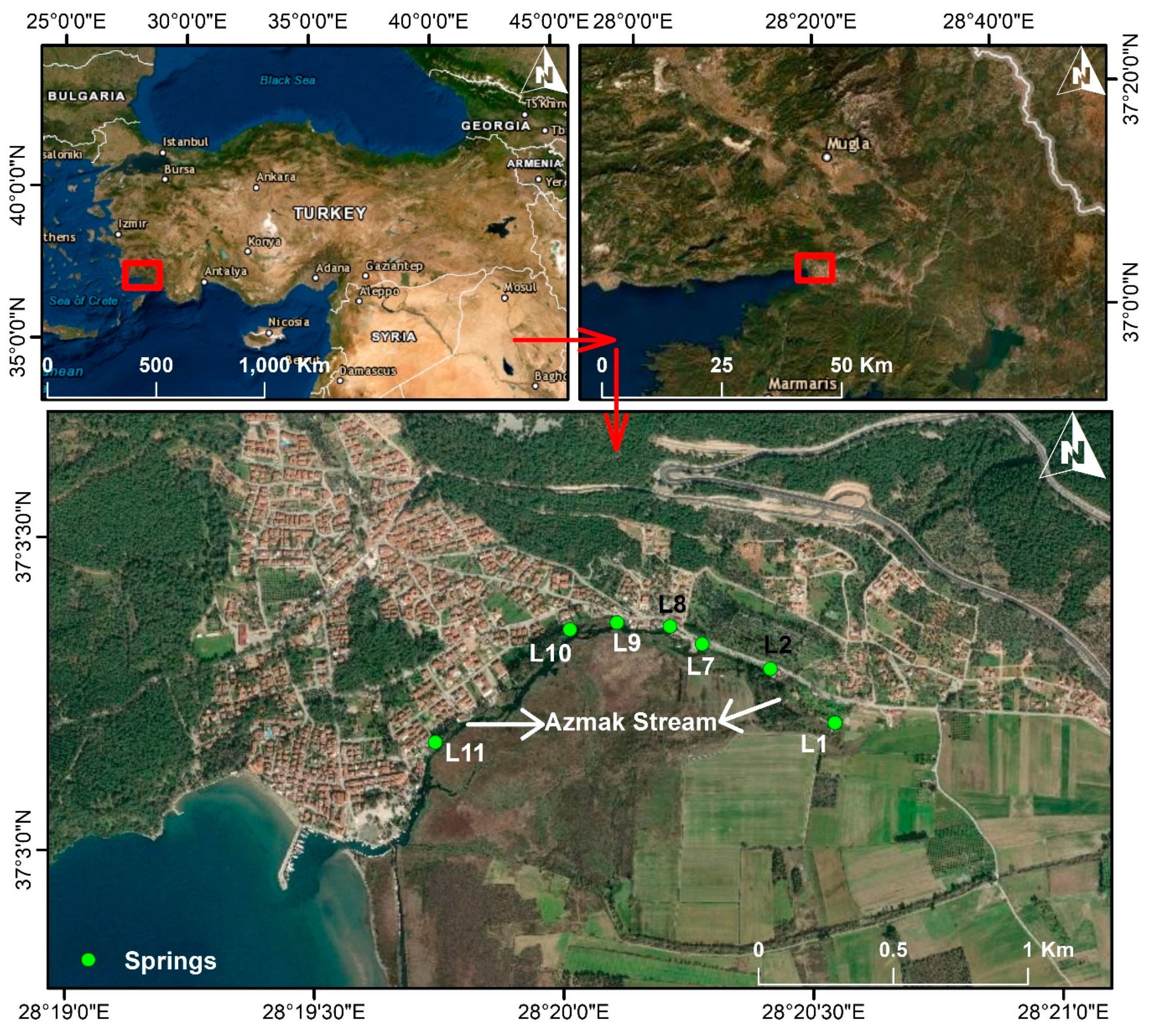
The name of the karst spring group in the Gökova Bay is the Azmak springs. Akyaka, the neighborhood where the Azmak springs are located, is a part of the Gökova Bay. The Azmak spring group also creates a stream called Azmak. The 2 km long Azmak Stream discharges to the Gökova Bay, Aegean Sea (Figure 1). The Gökova Bay is designated as a special environmental protection area by the Republic of Turkey Ministry of Environment and Forests in 1988.
Although the altitude is quite variable in the province of Mugla, the elevation of the plains in the study area is between 600–650 m above the sea level (ASL) and the peaks vary between 800–900 m ASL. The Azmak Stream and the springs have an elevation between 0 and 10 m ASL. According to Turkish State Meteorological Service, there is a Mediterranean climate in areas between 0 and 800 m of elevation ASL, and Mediterranean mountain climate at higher elevations. The average annual rainfall is slightly over 1100 mm. Most of the precipitation falls in winter-spring and drought occurs in summer.
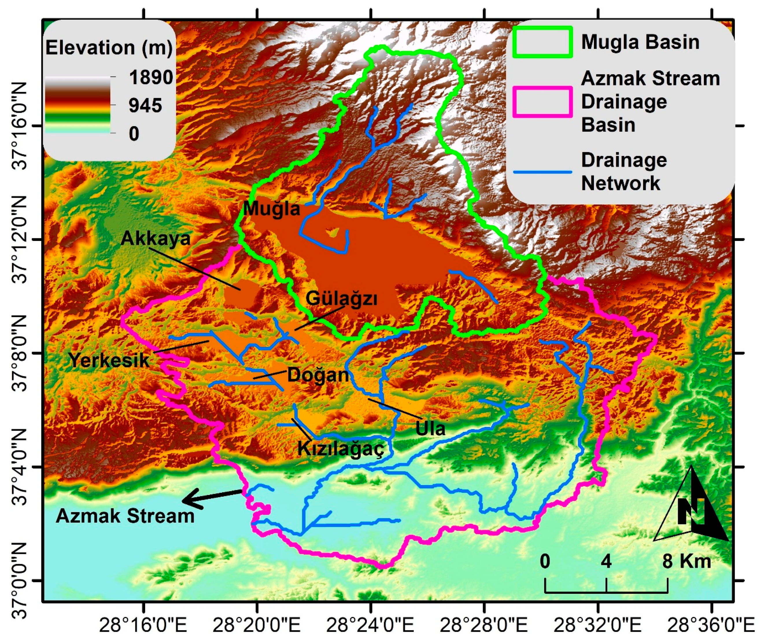
The Gulf of Gökova, where the Azmak Stream discharges, was formed as a result of a horst-graben system. The karst springs forming the Azmak Stream developed at the edge of the graben, the south of the horst. Akyaka, where the springs are in, is located on the hillside of a sharp elevation caused by the horst structure. The Azmak Stream is predominantly fed from karst aquifer, which has a 497 km2 surface drainage basin (Figure 2). The Mugla city center and Mugla Plain (also called Karabaglar Plateau) region are not in the surface drainage basin of Azmak Stream. Karabaglar Plateau is a closed basin (Figure 2). In the literature, several studies investigated the hydrogeology of the area and the Azmak springs. Kurttaş [33] calculated the hydrological budget, revealing that there is additional input from the neighboring basin from the north (Mugla city center and Mugla Plain). In other words, the Mugla basin is in karstic connection with the Azmak springs. Kurttaş et al. [34] and Bayarı and Kurttaş [35] determined the undersea discharge points of the karstic springs on the coast of Gökova by using satellite remote sensing techniques and hydrological budget. Bayarı et al. [36] studied the recovery of freshwater discharges and the detection of cold-water points along the Mediterranean coast including the Gulf of Gökova by different techniques. Ekmekçi et al. [37] worked on the determination of seawater mixture in Gökova karstic springs by hydrochemical and stable isotope methods. They proposed that syphon and venturi processes are effective for saltwater intrusion for the Azmak springs. Acikel et al. [38] and Açıkel [39] formed the conceptual model of Gökova karstic springs using hydrogeology, hydrochemical and environmental isotopes. Additionally, in this conceptual model, the Mugla basin was included in the drainage basin of the springs. Acikel and Ekmekci [40] used multivariate statistical methods to evaluate groundwater quality of Azmak Springs. They suggested that the springs waters are divided into 3–4 groups created by the seawater intrusion effect and freshwater contribution. Yıldıztekin and Tuna [41] investigated the irrigation water quality of the well waters in the Mugla Basin and they found that the groundwater pollution was not a serious issue in the area. Sağir and Kurtuluş [42] demonstrated the performance of empirical Bayesian kriging and geo-adaptive neuro-fuzzy inference system on the Mugla Basin alluvium by revealing the covered/alluvium filled dolines in the area. Kurtuluş et al. [43] also studied on the groundwater of the Mugla Basin alluvium to assess the metal(loid) contamination. Yet, there is not any study evaluating the development level of the karst system.
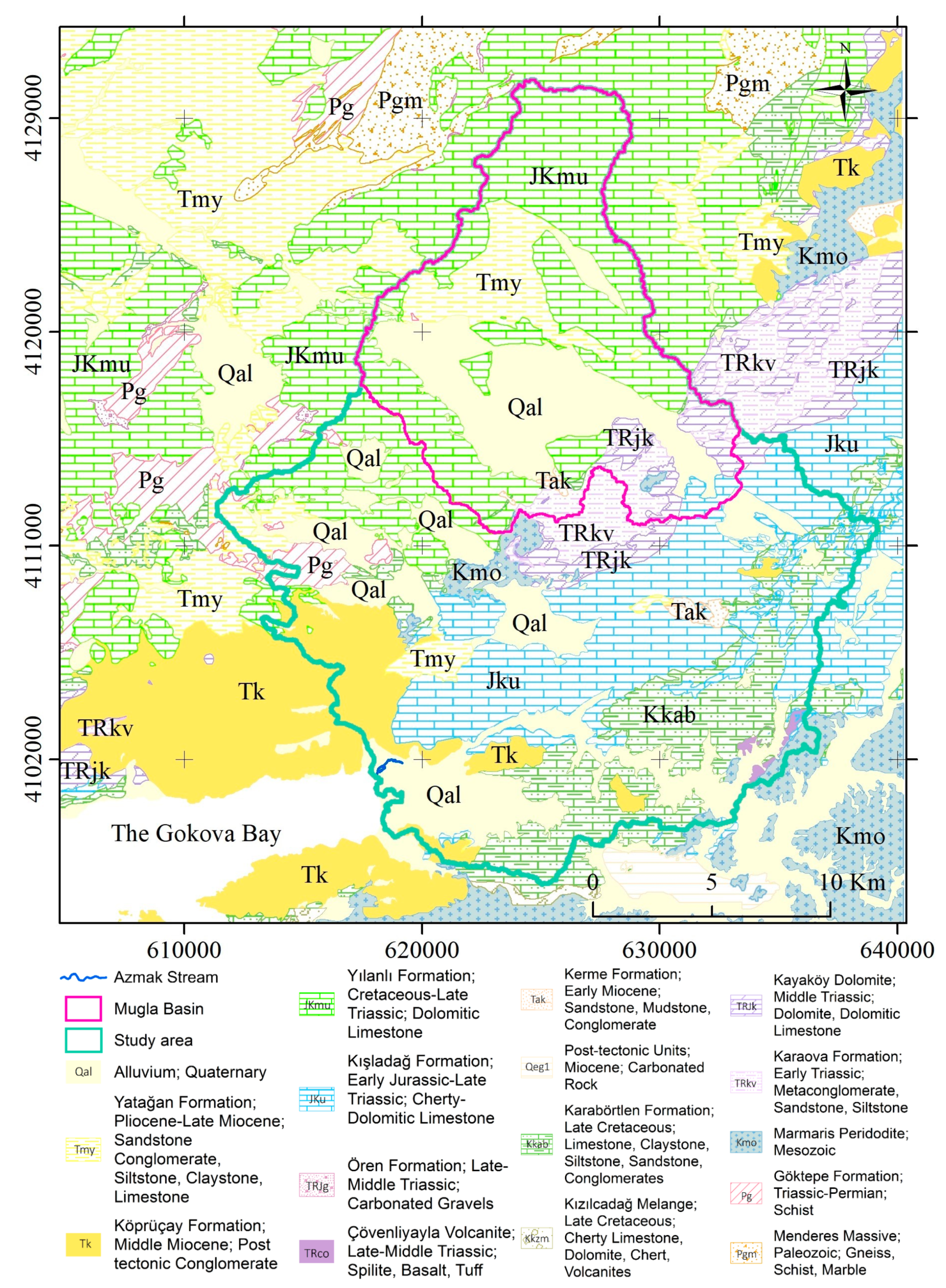
The geological map of the area was digitalized after the MTA (General Directorate of Mineral Research and Exploration) geological map of Turkey (Figure 3) [44]. The most important geological units in which the karstification has developed are the Cretaceous-Late Triassic dolomitic limestone (JKmu) and the Early Jurassic-Late Triassic cherty dolomitic limestone (JKu). The JKmu outcrops at north and northwest of the area around Mugla, Akkaya and Yerkesik-Dogan plains while the JKu outcrops at the center and the east around Ula and Kizilagac plains. In Akyaka, mostly colluvium is present, and its contact with Middle Miocene aged post-tectonic conglomerate (Tk) can be seen. Additionally, JKu outcrops just over the springs in some places. Triassic-Permian schist (Pg) and Mesozoic peridotite (Kmo) outcrop at the center which has hydrogeological importance. Kmo is a part of Lycian nappes thrust that underlies JKu and overlies JKmu. The thickness of the Quaternary alluvium (Qal) in the plains is up to 100 m.
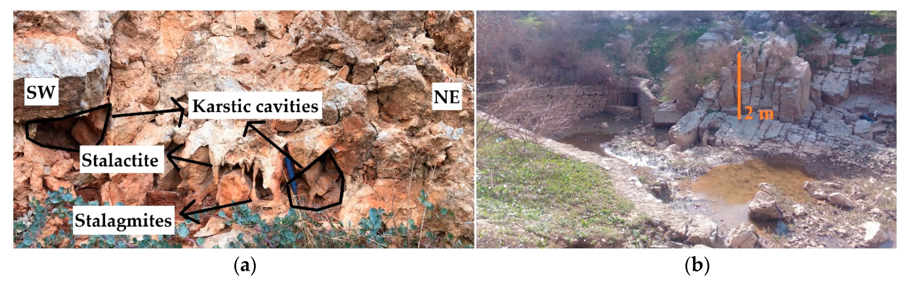
The most important factor of the region’s hydrogeology is the karstification of the carbonate rocks in the study area. The region shows most of the typical karst structures (Figure 4). Firstly, karst plains are important recharge areas in the region. The Mugla Plain is a closed basin, there is no stream coming out of the basin and all the water flows out of the basin as groundwater. Large and small karst structures are observed in all limestone-dolomite containing units in the region. The existence of sinkholes in all these plains is also known. The study region is quite active in tectonics, which creates faults, joints and fractures. These structural elements provided a favorable environment for karstification in the region where also rainfall is abundant. Since the horst-graben system in the region increases the hydraulic load difference between the recharge and discharge zones, it rules the groundwater flow and contributes to karstification. It can be suggested that the water drained in the Mugla Plain flows into the underground. Then, it is transferred through the southwest and Akkaya and Gulagzi Plains as groundwater flow. However, there is a low probability of groundwater flow from Mugla Plain to Ula Plain. The geological units can be cited as the reason for this. It is predicted that the Lycian Nappe thrust between the two plains prevents the groundwater flow. The Lycian Nappe unit, the Cretaceous peridotite and the serpentinized ophiolite are not suitable for groundwater flow. The Early Triassic metaconglomerate, sandstone, and siltstone unit (TRkv) in the same area is also impermeable. It is evaluated that the Lycian Nappe thrust continued towards the southwest of the region and was overlain by Middle Miocene post-tectonic conglomerate (Tk).
2.2. Data
Onset HOBO U20L-04 automatic data loggers were used for the water level measurements in the springs. This device can measure the water level between 0 and 4 m with ±0.4 cm accuracy and 0.14 cm resolution. The device can also measure the water temperature with an accuracy of ±0.44 °C and with a resolution of 0.1 °C. There are over 40 springs forming the Azmak Stream. However, the water level loggers were placed in L2 and L8 springs. L2 and L8 were chosen according to their temperature and electrical conductivity values measured over two years. These two springs showed different variations with time. Additionally, the rate of the discharges was enough during all the year when lots of the other springs dried out. The device placed at the L2 spring collected data between 02.09.2016–15.04.2018, and the device placed at the L8 spring collected data between 05.04.2017–05.02.2018. All the dates are given in dd.mm.yyyy format. All the measurements were done in 1-h intervals. The devices did not run out of battery during the measurement periods. However, since the memory of the devices got full after a certain number of measurements, the devices were removed from the springs and connected to the computer to transfer the data collected. Then, the loggers were placed back to the springs within no more than 20 min.
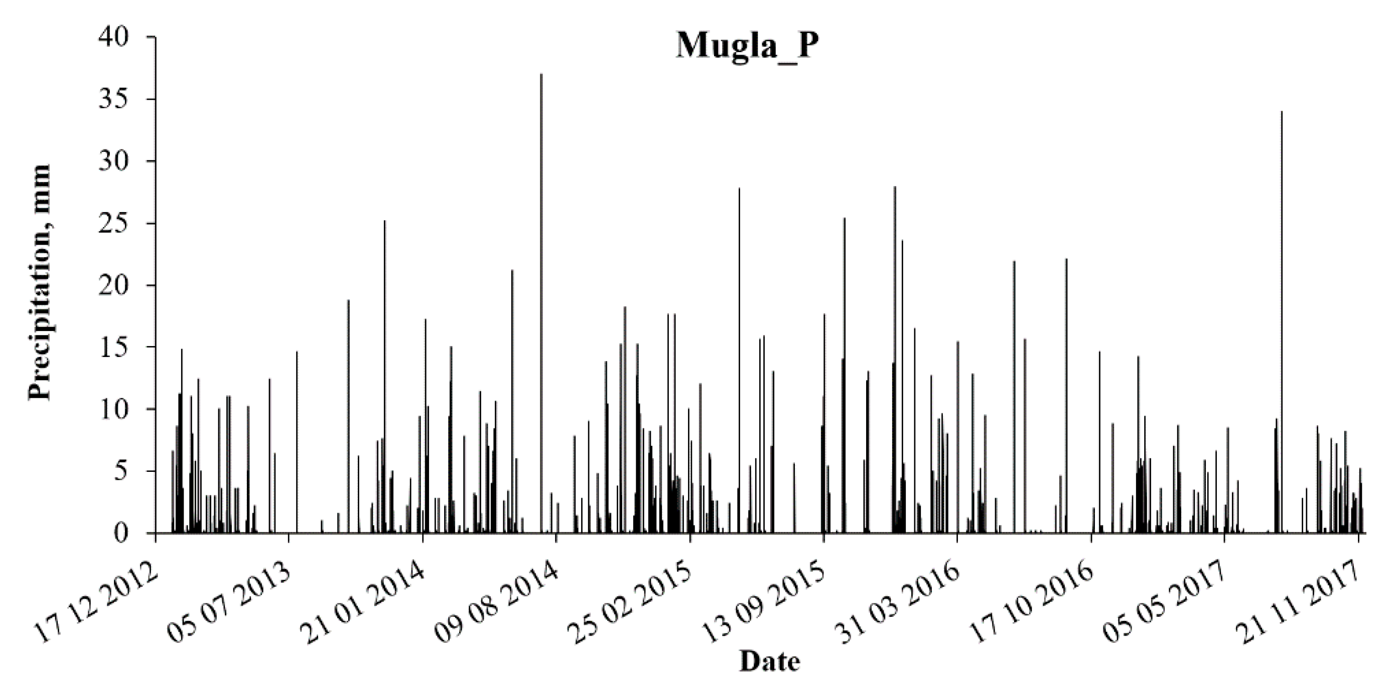
There are several weather stations near/in the study area. The rainfall data measured at the Mugla weather station represented the areal precipitation quite well. Açıkel [39] demonstrated that the regression is quite high (R2 = 0.99) between the data of the Mugla station and the stations nearby. The Mugla station rainfall data (P) is used in the study (Turkish State Meteorological Service). The hourly precipitation data is from 00:00 01.01.2013 to 22:00 06.12.2017 (Figure 5).
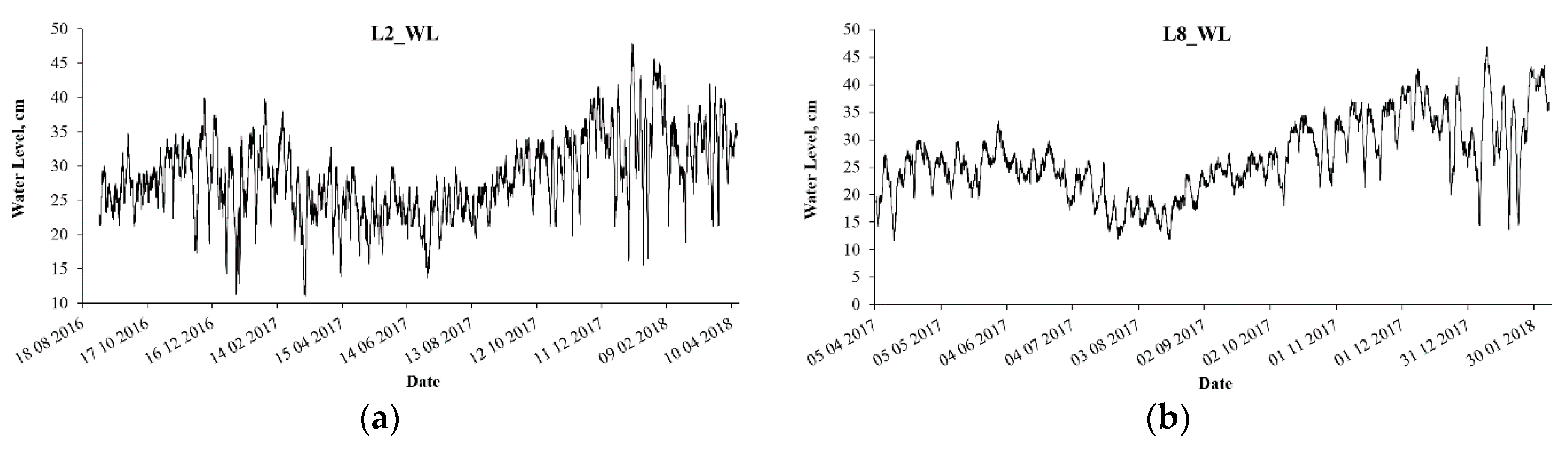
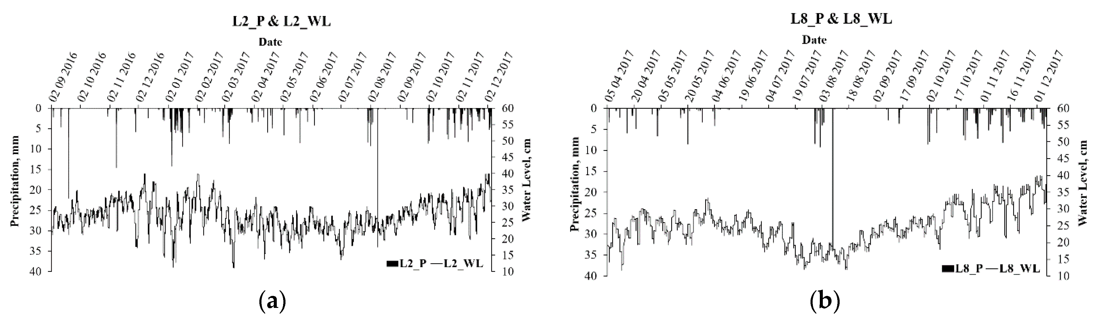
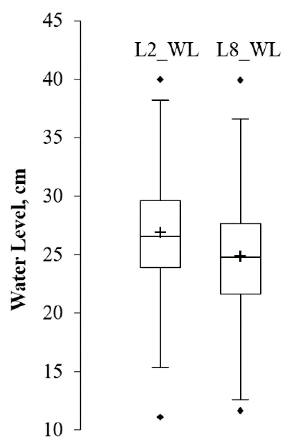
Hourly water level (from the water surface to the logger) data were measured at the springs. “0 level” corresponds to the altitude ASL of the spring location. The altitudes of the L2 and L8 are 12 and 9 m ASL, respectively. The L2 water level data is from 10:00 02.09.2016 to 07:00 15.04.2018 (Figure 6a). The L8 water level data is from 16:00 05.04.2017 to 18:00 05.02.2018 (Figure 6b). Intersections of the data were used since all data are not exactly overlapped. Statistical analyses between L2 precipitation (L2_P) and L2 water level (L2_WL) were performed for the data between 10:00 02.09.2016 and 00:00 06.12.2017 with the data length of 10110 (Figure 7a). Statistical analyses between L8 precipitation (L8_P) and L8 water level (L8_WL) were performed for the data between 16:00 05.04.2017 and 00:00 06.12.2017 with the data length of 5509 (Figure 7b). General descriptive statistics and the box plot for L2_WL and L8_WL data are given in Table 1 and Figure 8.
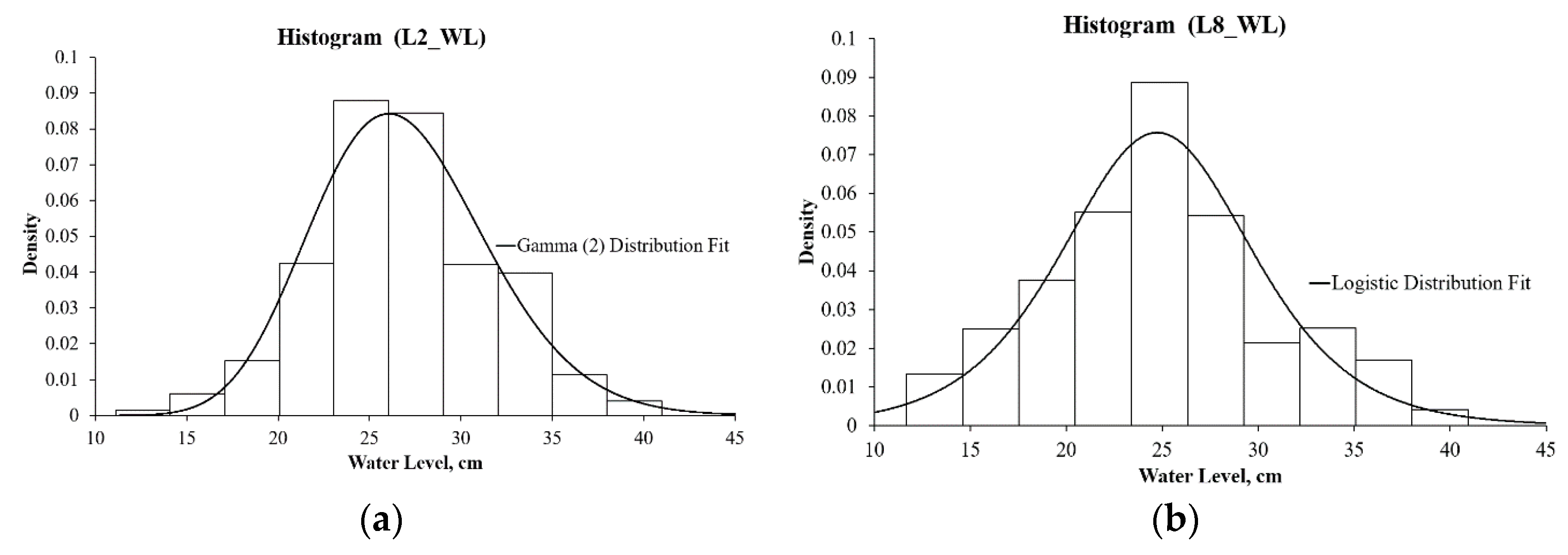
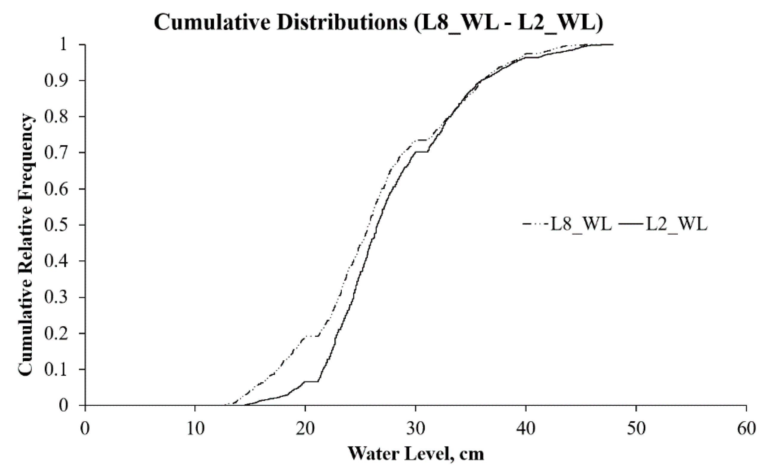
Distribution fitting and cumulative distribution fitting comparison for the L2_WL and L8_WL data were investigated in order to find out the statistical distribution characteristics and the similarities of the data. Distribution fittings were done by using maximum likelihood estimation with a 5% significance level. The L2_WL data were best fitted to Gamma-2 type distribution with the p-value of 3.08 × 10⁻¹⁴ (Figure 9a). The L8_WL data were best fitted to logistic type distribution with the p-value of 1.80 × 10⁻¹¹ (Figure 9b). The cumulative distributions of the L2_WL and the L8_WL data were compared by the two-sample Kolmogorov-Smirnov test with the significance level of 5% (Figure 10). The p-value was found lower than 0.0001, which indicates that the distributions of the data are not identical. Thus, using these two datasets to make different interpretations is significative.
2.3. Method
2.3.1. Recession Coefficient
All the calculations in this paper were carried out on Microsoft Excel with XLSTAT add-in.
Spring water level data were used for recession analyses to achieve a better understanding of the hydrodynamic properties of the karst aquifer. Since the data is hourly, monthly moving average values were used to demonstrate a clearer view of the data. Then, recession coefficient calculations performed using the Maillet [46] equation given in Equation (1):
- α: Recession coefficient (1/day, multiplied by 24 for the conversion from hour to day)
- Qt: Flow rate at the time t (Water-level in cm was used.)
- : The last flow rate before the recession (Water-level in cm was used.)
- t: Recession duration (hours)
2.3.2. Simple/Autocorrelation and Simple Spectral Density Function
The simple correlation function is calculated by the following formula (Equation (2)) after Box et al. [47]:
- rk: Autocorrelation function
- k: Time lag, from 0 to m which is the cutting point
- C: Correlogram
- n: Length of the time series
- i: Time
- x: Parameter, water level
- : Mean value of the time series
Spectral density function S(f) (Equation (3)), corresponds to the change from a time mode (time series space) to a frequency mode by applying the Fourier’s transformation on the variables [47]. The cut-off frequency is the time lag when the S(f) of water quantity data gets the values lower than 1 and gets negligible. This means that the input (precipitation) events before the calculated time lag are filtered.
- S(f): Spectral density function
- F: is equal to j/2m
- j: is from 1 to m
Dk is a window being used to get an unbiased estimation of S(f). Mangin [2,3] suggested Tukey’s window as the best performing (Equation (4)):
The determining of the lag k and the truncation m is crucial for the correlation and the spectral analyses according to Mangin [2,3], who also suggested that it is much better to set an m value not higher than n/3, while n is the length of the time series. The value form is never selected to be higher than n/3 throughout this study.
2.3.3. Cross-Correlation and Cross-Spectral Density Functions
The cross-correlation function is calculated by the following formula after Larocque et al. [6] (Equation (5)):
- rx,y(k): Cross-correlation function
- Cx,y(k): Cross-correlogram
- σx: Standard deviation of the x time series
- σy: Standard deviation of the y time series
- : Mean value of the x time series
- : Mean value of the y time series
The higher degree of symmetry for the cross-correlogram graph indicates that there is another parameter affecting the variables. If the input signal is highly changed in the system, the maximum rx,y(k) gets a lower value. In the karst environment, this means that the karst system is more complex and not highly developed. The lag to the maximum rx,y(k) is called the delay which describes the transfer speed of the input change.
The cross-spectral density function, Sx,y(f) (Equations (6)–(8)), is the Fourier’s transformation of the cross-correlation function [6]:
where:
The coherence function COx,y(f) indicates the linearity of the input-output system (Equation (9)). The system is linear when the COx,y(f) near or equal to 1. High linearity is a signal of that any change in input has an analogical effect on the output. High linearity for karst systems’ input-output means well-developed karstification. Non-linearity shows there are other factors might be considered [6].
If the gain function gx,y(f) is higher than 1, there is an amplification of the output signal (Equation (10)). If the gain function gx,y(f) gets a value lower than 1, there is an attenuation of the output signal [6]. The time lag for the amplification indicates the delay of the water release from the karst storage. While the discharge is being characterized by the precipitation, releasing the reservoir water beside the input related discharge creates an amplification after a certain delay (time lag of the gain function). The presence of amplification may also indicate the high storage capacity of the karst system.
2.3.4. Karst Aquifer System Classification
Mangin [2,3] made a classification of karst aquifer systems in relation to the results of correlation and spectral analyses. This classification consists of four karsts that have been studied in detail before. This classification is based on four parameters: memory effect, spectral range, regulation time and unit hydrograph pattern (Table 2).
The memory effect is the time lag for the correlogram reaches the value of 0.2. It points out the fall of the speed of the correlation. Rapid decrease exhibits the quasi-randomness of the response. The slow decrease means that the response is well structured. The slow decrease of the correlation implies a higher memory effect. The higher memory effect reveals that the karst’s idle nature. Idle karsts are often related to large storage. Hence, a correlogram decreasing slowly defines the poorly-karstified (poorly drained) system.
The regulation time corresponds to the duration of the input influence on the output. Regulation time is calculated by dividing the maximum spectral density value by 2, referring to the results of the spectral density function.
The spectral range corresponds to the frequency value when the spectral density is equal to zero. Broad spectral range points well-drained karst systems.
By using the mentioned approaches and methods above, a general view of the material, the method and expected results are given in Table 3.
3. Results
3.1. Recession Coefficients
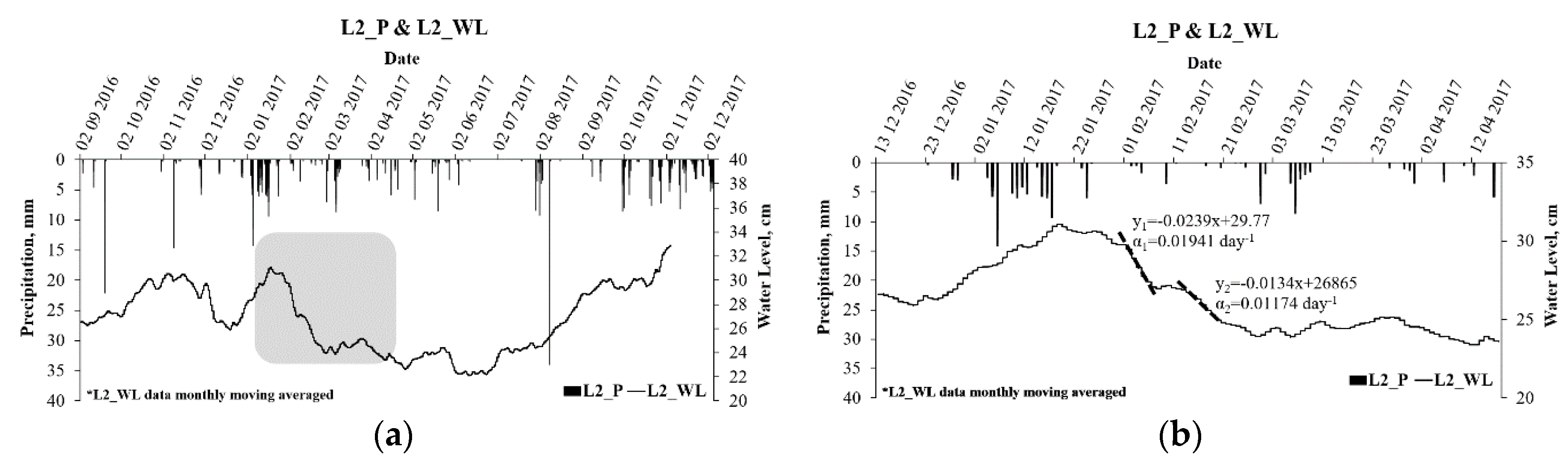
Two different recession coefficients for the L2_WL data were calculated in a selected period so that the water level is not disturbed by any rainfall (Figure 11a). The recession coefficients were calculated as 0.01941 day−1 and 0.01174 day−1 (Figure 11b). Two different coefficients indicate that the recession occurs in two phases. The first phase represents the respectively well-karstified zone (conduits/fractures) with higher transmissivity and hydraulic conductivity, and lower storage capacity. The second phase represents the respectively poorly karstified zone (matrix/fractures) with lower transmissivity and hydraulic conductivity, and higher storage capacity.
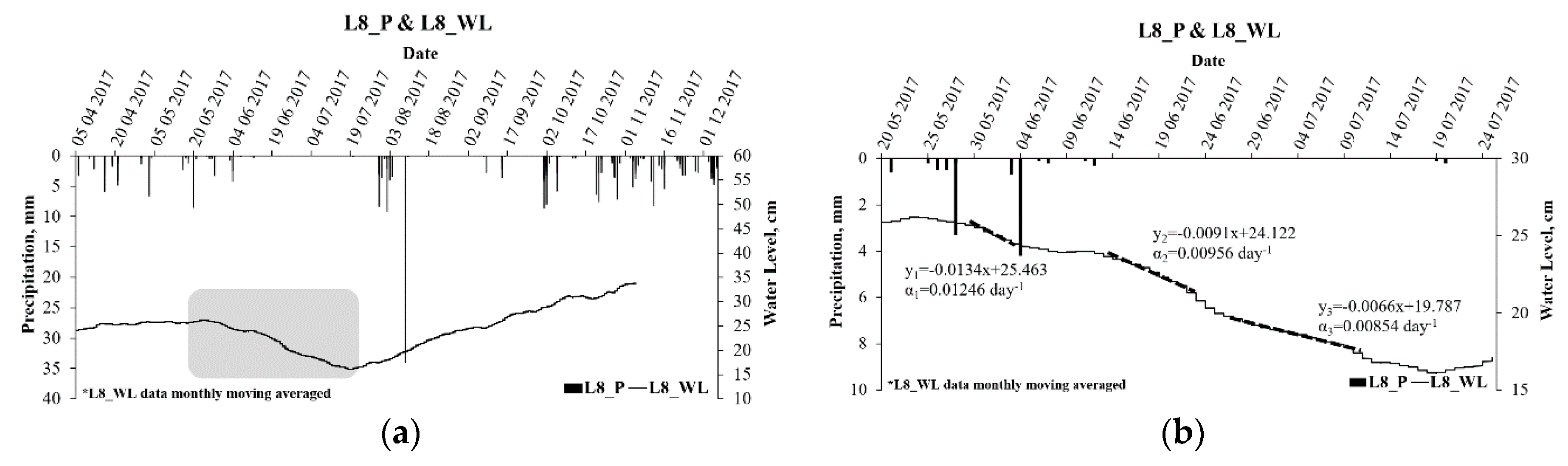
Three different recession coefficients for the L8_WL data were calculated in a selected period shown in Figure 12a. The recession coefficients were calculated as 0.01246 day−1, 0.00956 day−1 and 0.00854 day−1 (Figure 12b). Three different coefficients indicate that the recession occurs in three phases. The first phase represents the respectively well-karstified zone (conduits) with higher transmissivity and hydraulic conductivity and lower storage capacity. The second phase represents the medium karstified zone (fractures) with medium transmissivity, hydraulic conductivity and storage capacity. The third phase represents the porous medium (matrix) with lower transmissivity and hydraulic conductivity and higher storage capacity. For this spring, the presence of the third phase means that the epikarst and the alluvium plains have an important effect on the water level of the spring discharge.
3.2. Simple/Autocorrelation
L2_P and L8_P autocorrelogram are given in Figure 13a,b. Autocorrelation r(k) gets a value of 0.2 at the time lag of 3 h for the L2_P data. r(k) gets 0.2 at 2 h for the L8_P data. The time lag for r(k) gets 0.2 represents the memory effect of the data. Too fast memory effect is an indication that the data is an independent variable showing quasi-randomness.
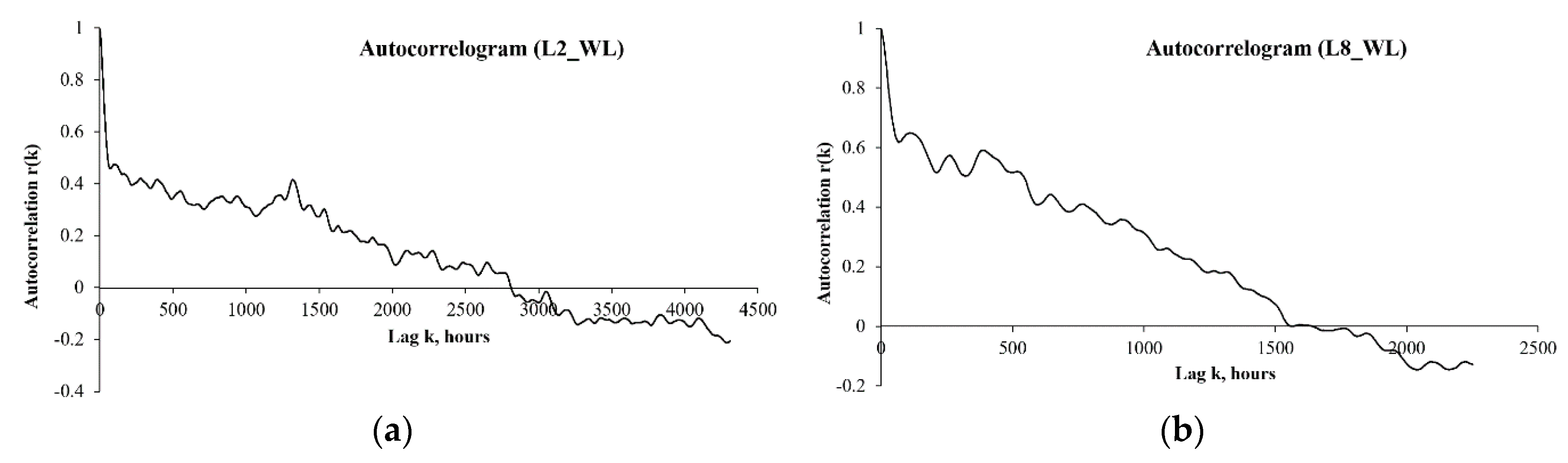
Autocorrelogram for the L2_WL and the L8_WL are given in Figure 14a,b. For the L2_WL, r(k) gets 0.2 at 1751 h, which makes 73 days as the memory effect. For the L8_WL, r(k) gets 0.2 at 1212 h which makes 51 days as the memory effect. Shorter the memory effect more developed the karstification. L2_WL memory effect is equal to 73 days, which is extensive and indicates poorly drained and karstified Torcal type karst aquifer (Table 2). The L8_WL memory effect of 51 days is large, which indicates better drained and karstified aquifer (Fontestorbes type) than the L2_WL. Moussu [48] listed the karst systems of Fontaine de Chartreux, Fontaine de Vaucluse and Durzon having the memory effects as 71, 75 and over 100 days, respectively. Lorette et al. [49] indicated 77 days of memory effect for Toulon spring.
3.3. Simple Spectral Density Function
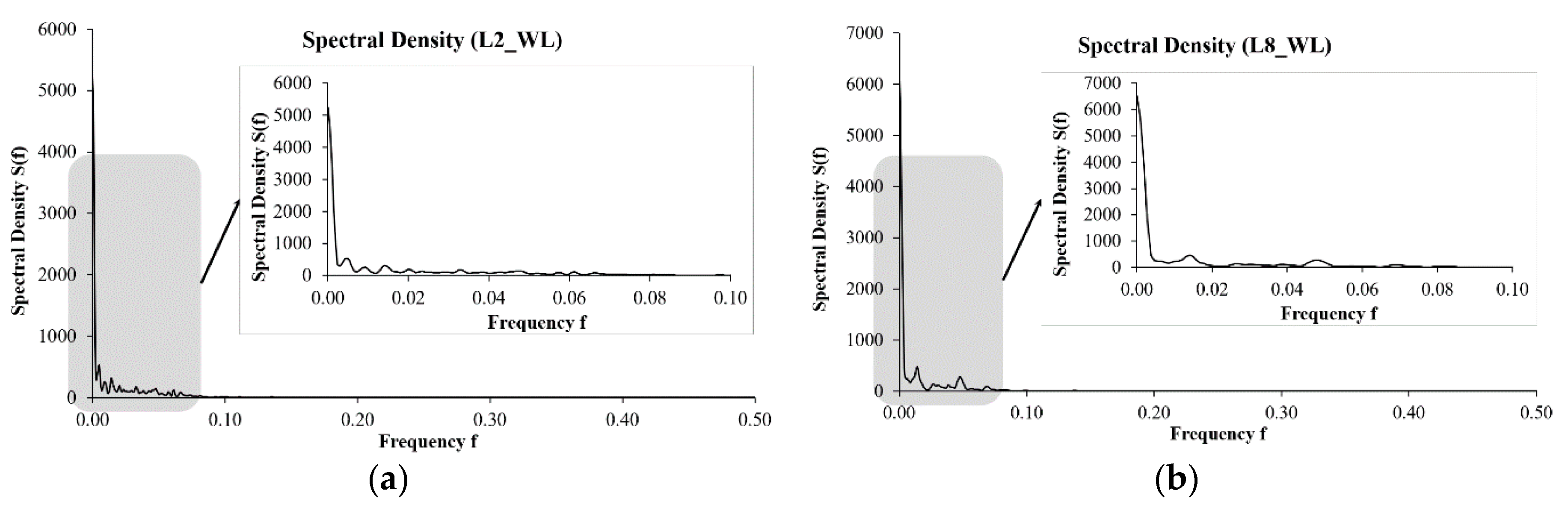
The simple spectral density function for the L2_WL and the L8_WL are given in Figure 15a,b. S(f0) values are 5233 and 6508 for the L2_WL and L8_WL respectively. For L2_WL data spectral range is lower than 0.1 and the regulation time is 109 days. For L8_WL data spectral range is again lower than 0.1 and the regulation time is 136 days. The cut-off frequencies are 3.1 and 3.5 days for the L2_WL and L8_WL respectively. This means that the rainfall takes place no longer than 3–3.5 days is being filtered by the karst aquifer system, and no effects of those rainfall events on the discharge can be detected. For both data, the spectral ranges are very narrow and the regulation times are too long, which are the indications of the Torcal type poorly drained and karstified aquifers. The classification points a much more poorly karstified aquifer than the Torcal since the parameters’ values are not very close to the Torcal type.
3.4. Cross-Correlation Function
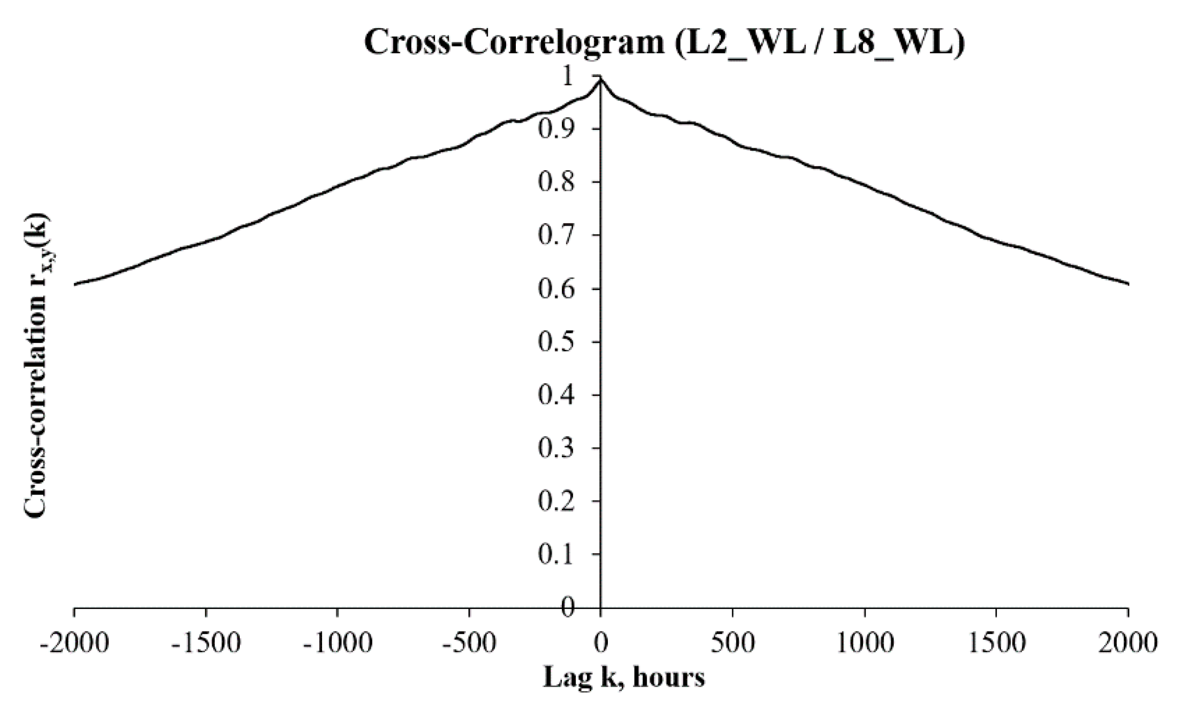
The cross-correlogram between L2 and L8 water level data is given in Figure 16. The highly symmetrical plot of the cross-correlation for the L2 vs. L8 water level data indicates that there is a common input and the reaction against that input of these two data is similar.
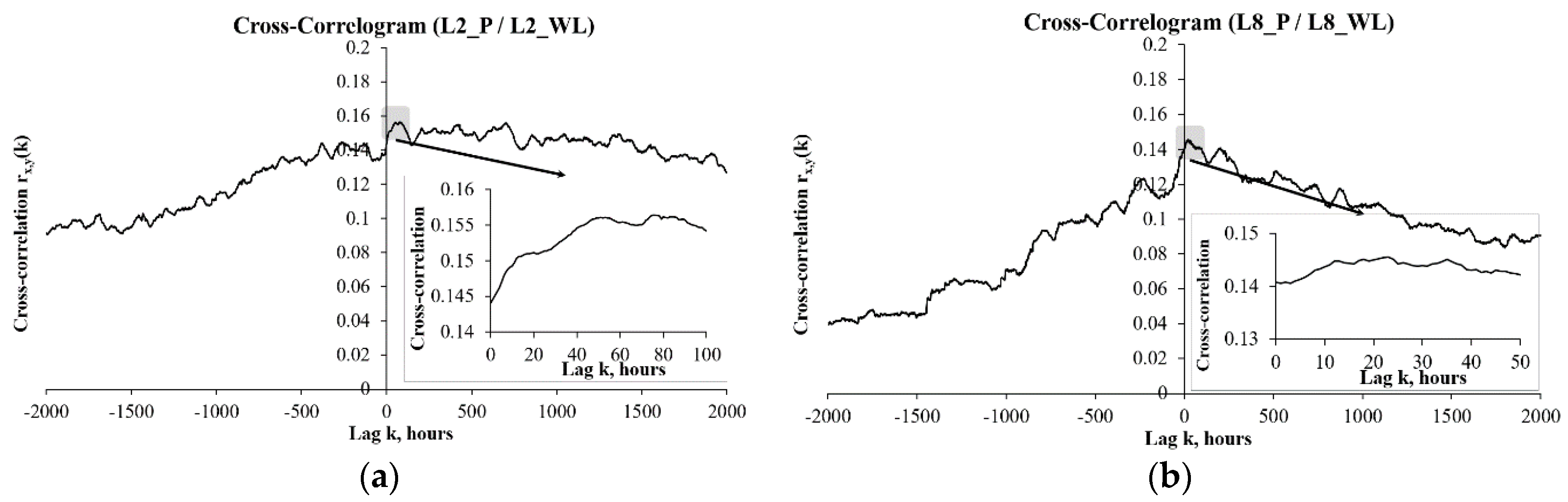
The cross-correlograms of precipitation versus L2 and L8 water level data are given in Figure 17a,b respectively. Cross-correlation function for precipitation versus L2 and L8 discharge demonstrated a dissymmetrical plot, which is the mark of influence of the input (precipitation) on the output (discharge). The maximum cross-correlation values for L2 and L8 were calculated as 0.1564 and 0.1455, respectively. The low degree of the maximum rx,y(k) values for the springs showed that the input was highly changed throughout the output. Slightly lower values for L8 might be the indication of a more complex recharge system.
“The delay” described as the transfer speed and corresponds to the time lag to the maximum rx,y(k). The shorter delay indicates the faster transfer of the input influence on the output. The delays were 24 and 76 h for L8 and L2 respectively. To compare, Larocque et al. [6] calculated 0.5–0.8 for maximum rx,y(k) values and 12–17 h of delay for a karst system, which had approximately 75 days of regulation time. Lo Russo et al. [50] calculated 1, 1, 1 and 38 days for different springs, which have 49, 57, 63 and 52 days of memory effect, respectively. Additionally, Fu et al. [51] calculated the 1-day delay for a discharge with a memory effect of 4 days. Thus, the signal transfer speed of the system is quite low which indicates a low degree of karstification.
3.5. Cross-Spectral Density Function
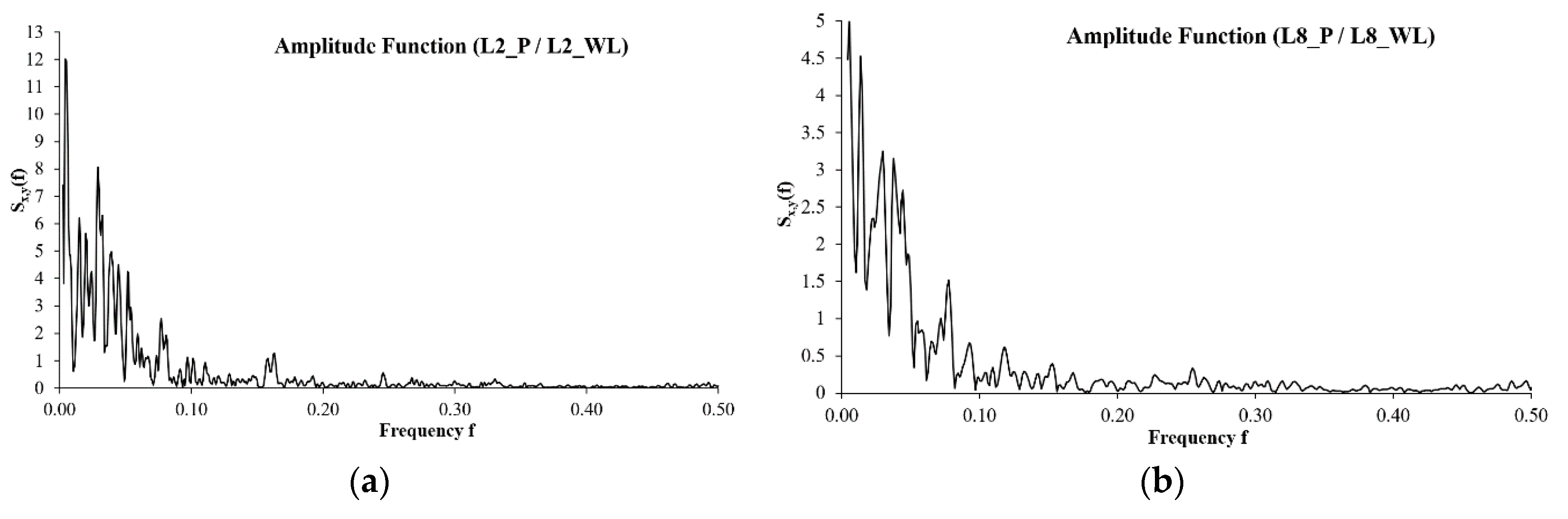
The amplitude functions (cross-spectral densities) for the L2_P-L2_WL and the L8_P-L8_WL are given in Figure 18a,b. Cut-off frequencies are 6.1 and 12.5 days for the L2_P-L2_WL and the L8_P-L8_WL. These values are quite high in comparison with Bange-L’Eau-Morte of 4.5 days [16] and Ain Zerga of 5 days [21]. This shows that the Mugla karst has quite inertial behavior.
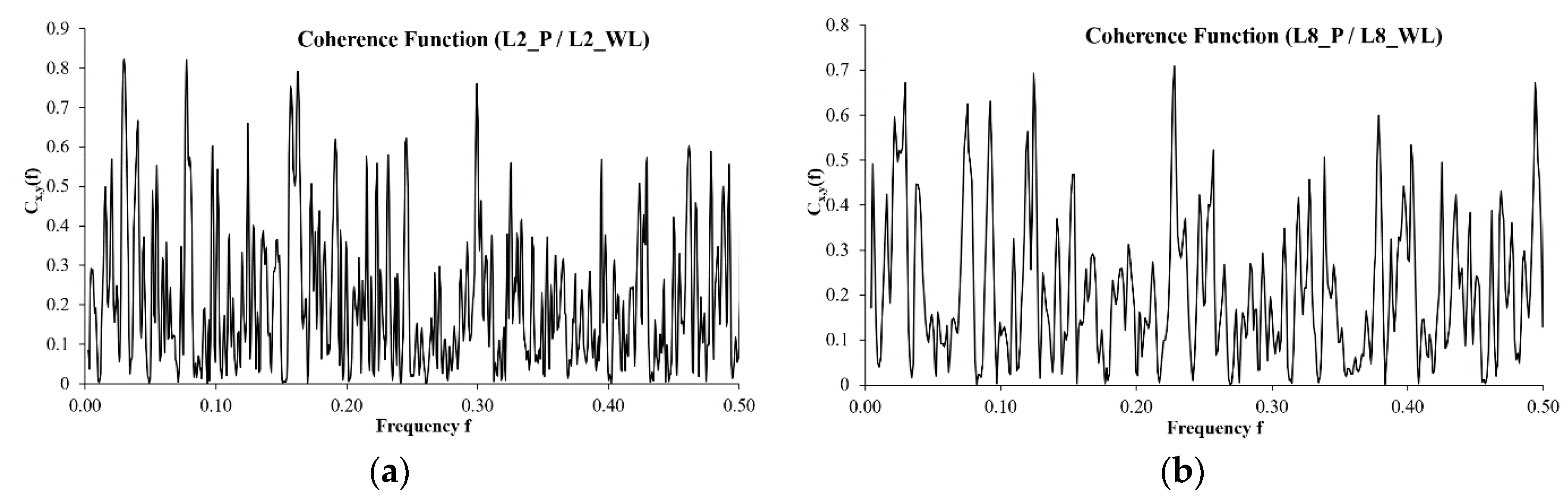
The coherence functions for the L2_P-L2_WL and the L8_P-L8_WL are given in Figure 19a,b. The average coherence values are 0.21 for both L2 and L8. Low coherence means the non-linearity for the input-output system, and non-linearity might be a sign of poor karstification.
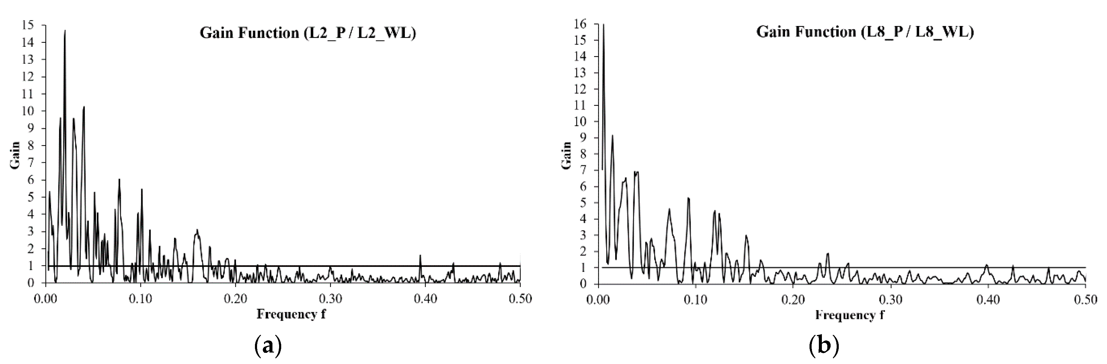
The gain functions for the L2_P-L2_WL and the L8_P-L8_WL are given in Figure 20a,b. For both data set, the gain functions are dominantly higher than 1 up to the 0.1 frequency. The amplifications occur almost at every frequency which shows that the karst system has high storage capacity because the system discharges the reserve water even at later frequencies. There are also the amplifications at mid frequencies indicating that there is very strong late infiltration.
4. Discussion and Conclusions
Correlation and spectral analyses were applied to the data of Mugla precipitation and the water level of two springs with the intent to achieve hydrodynamic properties of the karst aquifer. The karstification level/development of the karst and its internal parts were evaluated. The methods and the outputs are discussed as the same order as they were given in Table 3. All the expected outputs were achieved, even when the water level data were used instead of flow rate.
Hydrograph analysis were done using water level data of the two spring. The recession analysis in this paper was only used to discriminate the different number of phases for the springs if there are any. Since the used data are water levels of the springs, the calculated recession coefficients do not bear any physical sense compared to recession coefficients derived from flow rates analysis. The purpose was to show the different recession phases for the springs, which is important for understanding the system functioning. A complete recession analysis should split the flood flow and the base flow. However, in this paper, this is not the case, because there is no effective rain after the starting point of the recession. For that period, for L2, there are about five rain events with an average of 1–2 mm. For L8, it is more or less the same situation with a slightly higher amount of rain, of 2–3 mm. Taking into account the fact that the numerical values of the recession coefficients are not significant, the rainfall amount in the period of recession is already negligible to consider the infiltration effect. According to Mangin [52], the infiltration effect can be neglected under these kinds of conditions. In order to calculate the dynamic volume, storage and hydraulic conductivity through the recession curve, flow rate data are required. Thus, it was not possible to calculate these parameters using conventional methods with water level data. Horoi [27] also used the water level data instead of discharge rate data of the springs for the statistical analyses. Since most of the calculations are unitless, this may not cause any error. However, the relation between the water level and the flow rate is not proportional. This issue should be addressed by further investigations comparing these two kinds of data for the same discharge. Considering the recession analysis, karst internal parts were grouped as matrix (alluvium plains/dolines/poljes), fractures (poorly karstified zone) and conduits (well-karstified zone). For the L2 spring, only matrix and fracture parts of the karst were determined. For the L8 spring, all three main parts of the karst were detected. The calculated recession coefficients might indicate poorly developed conduit structure and a low degree of karstification.
The uncertainty caused by the use of the water level data instead of the flow rates is also valid for the correlation and the spectral analyses results. However, in these analyses, the calculations and their values bear physical sense. The calculated values are in accordance with those in the literature. Autocorrelation and simple spectral calculations using water level data provided memory effect, spectral range, regulation time and cut-off frequencies. Cross-correlation and cross-spectral calculations using the precipitation and the water level data provided delay, degree of correlation, linearity of the system, storage capacity and late infiltration effect. Water level data were used for all these calculations also. Yet, the results were consistent with each other and those in the literature and had hydrogeological meanings, which indicated a low degree of karstification for the studied karst system. According to the correlation and spectral analyses, the response (spring discharge) of the input (precipitation) is slow, non-linear and well modified, which are again the signs of poor karstification. Yet, the karst aquifer has high storage capacity and a strong late infiltration effect. The important late infiltration effect stands for the dominant role of the matrix zone.
In light of the findings on the Mugla karst system, it can be suggested that the karst development level of this system is low. It can be concluded that the epikarst and the alluvial plains are still the most important parts of this karst system. The Mugla karst system is a vital water resource for the region. It is therefore essential to pay more attention to these parts of the karst system while managing it in a sustainable way. Considering the revealed features of the karst system, it is not possible to create sudden floods in the discharge area, but attention should be paid to the flooding that may occur due to late drainage of water in the feeding area.
Author Contributions
Conceptualization, B.K. and M.R.; Methodology, Ç.S.; Software, Ç.S.; Validation, B.K. and M.R.; Formal analysis, Ç.S.; Investigation, Ç.S. and B.K.; Resources, B.K.; Data curation, Ç.S.; Writing—original draft preparation, Ç.S.; Writing—review and editing, B.K., M.R. and Ç.S.; Visualization, Ç.S.; Supervision, B.K. and M.R.; Project administration, B.K. and M.R.; Funding acquisition, B.K. and M.R. All authors have read and agreed to the published version of the manuscript.
Funding
This research was funded by the Scientific Research Project Office of Mugla Sitki Kocman University, grant number 16/029.
Acknowledgments
The authors are grateful to Günseli ERDEM and Ersin ATEŞ for their support on the field works. The authors thank the editor and the anonymous reviewers.
Conflicts of Interest
The authors declare no conflict of interest. The funder had no role in the design, execution, interpretation or writing of the study.
References
- Box, G.E.; Jenkins, G.M. Time Series Analysis: Forecasting and Control; Holden-Day Inc.: San Francisco, CA, USA, 1970; p. 553. [Google Scholar]
- Mangin, A. Pour une Meilleure Connaissance des Systèmes Hydrologiques à Partir des Analyses Corrélatoire et Spectrale. J. Hydrol. 1984, 67, 25–43. [Google Scholar] [CrossRef]
- Mangin, A. Karst Hydrogeology. In Groundwater Ecology; Gibert, J., Danielopol, D.L., Stanford, J.A., Eds.; Academic Press Limited: London, UK, 1994; pp. 43–67. [Google Scholar]
- Padilla, A.; Pulido-Bosch, A.; Mangin, A. Relative importance of Baseflow and Quickflow from Hydrographs of Karst Spring. Groundwater 1994, 32, 267–277. [Google Scholar] [CrossRef]
- Eisenlohr, L.; Király, L.; Bouzelboudjen, M.; Rossier, Y. Numerical simulation as a tool for checking the interpretation of karst spring hydrographs. J. Hydrol. 1997, 193, 306–315. [Google Scholar] [CrossRef] [Green Version]
- Larocque, M.; Mangin, A.; Razack, M.; Banton, O. Contribution of correlation and spectral analyses to the regional study of a large karst aquifer (Charente, France). J. Hydrol. 1998, 205, 217–231. [Google Scholar] [CrossRef]
- Bakalowicz, M. Karst groundwater: A challenge for new resources. Hydrogeol. J. 2005, 13, 148–160. [Google Scholar] [CrossRef]
- Panagopoulos, G.; Lambrakis, N. The contribution of time series analysis to the study of the hydrodynamic characteristics of the karst systems: Application on two typical karst aquifers of Greece (Trifilia, Almyros Crete). J. Hydrol. 2006, 329, 368–376. [Google Scholar] [CrossRef]
- Bakalowicz, M.; El Hakim, M.; El-Hajj, A. Karst groundwater resources in the countries of eastern Mediterranean: The example of Lebanon. Environ. Geol. 2008, 54, 597–604. [Google Scholar] [CrossRef]
- Moussu, F.; Oudin, L.; Plagnes, V.; Mangin, A.; Bendjoudi, H. A multi-objective calibration framework for rainfall–discharge models applied to karst systems. J. Hydrol. 2011, 400, 364–376. [Google Scholar] [CrossRef]
- Fiorillo, F.; Doglioni, A. The relation between karst spring discharge and rainfall by cross-correlation analysis (Campania, Southern Italy). Hydrogeol. J. 2010, 18, 1881–1895. [Google Scholar] [CrossRef]
- Hartmann, A.; Barberá, J.A.; Lange, J.; Andreo, B.; Weiler, M. Progress in the hydrologic simulation of time variant recharge areas of karst systems–Exemplified at a karst spring in Southern Spain. Adv. Water Resour. 2013, 54, 149–160. [Google Scholar] [CrossRef]
- Kovács, A.; Sauter, M. Modelling karst hydrodynamics. In Methods in Karst Hydrogeology; Goldscheider, N., Drew, D., Eds.; CRC Press: London, UK, 2014; pp. 215–236. [Google Scholar]
- Pulido-Bosch, A.; Padilla, A.; Dimitrov, D.; Machkova, M. The discharge variability of some karst springs in Bulgaria studied by time series analysis. Hydrol. Sci. J. 1995, 40, 517–532. [Google Scholar] [CrossRef]
- Jeannin, P.Y.; Sauter, M. Analysis of karst hydrodynamic behaviour using global approaches: A review. Bull. Hydrogéol 1998, 16, 31–48. [Google Scholar]
- Mathevet, T.; Lepiller, M.; Mangin, A. Application of time-series analyses to the hydrological functioning of an Alpine karstic system: The case of Bange-L’Eau-Morte. Hydrol. Earth Syst. Sci. Discuss. 2004, 8, 1051–1064. [Google Scholar] [CrossRef]
- El Hakim, M. Les Aquifères Karstiques de l’Anti-Liban et du nord de la Plaine de La Bekaa: Caractéristiques, Fonctionnement, Evolution et Modélisation, d’Après l’Exemple du Système Karstique Anjar-Chamsine (Liban). Ph.D. Thesis, University of Montpellier II, University of Saint Joseph, Montpellier, France, Beirut, Lebanon, 2005. [Google Scholar]
- Massei, N.; Dupont, J.P.; Mahler, B.J.; Laignel, B.; Fournier, M.; Valdes, D.; Ogier, S. Investigating transport properties and turbidity dynamics of a karst aquifer using correlation, spectral, and wavelet analyses. J. Hydrol. 2006, 329, 244–257. [Google Scholar] [CrossRef]
- Salerno, F.; Tartari, G. A coupled approach of surface hydrological modelling and Wavelet Analysis for understanding the baseflow components of river discharge in karst environments. J. Hydrol. 2009, 376, 295–306. [Google Scholar] [CrossRef]
- Bailly-Comte, V.; Martin, J.B.; Screaton, E.J. Time variant cross correlation to assess residence time of water and implication for hydraulics of a sink-rise karst system. Water Resour. Res. 2011, 47. [Google Scholar] [CrossRef] [Green Version]
- Hemila, M.L.; Guefaifia, O.; Gouaidia, L.; Djoulah, B. Characterizing Functioning of the Dyr Karst (Tebessa, Algeria) by Correlative and Spectral Analysis of Hydro-Pluviometric Chronicles. In Proceedings of the EuroKarst 2016, Neuchatel, Switzerland, 5–7 September 2017; pp. 193–202. [Google Scholar]
- Pavlić, K.; Parlov, J. Cross-Correlation and Cross-Spectral Analysis of the Hydrographs in the Northern Part of the Dinaric Karst of Croatia. Geosciences 2019, 9, 86. [Google Scholar] [CrossRef] [Green Version]
- Atalay, İ. Potential and problems of karstic fields. In Proceedings of the 15th Scientific and Technical General Assembly of Geomorphology of Turkey, Ankara, Turkey, 20–24 April 1998; pp. 3–4. [Google Scholar]
- Ekmekci, M. Review of Turkish karst with emphasis on tectonic and paleogeographic controls. Acta Carsol. 2003, 32, 205–218. [Google Scholar]
- Bayari, C.S.; Ozyurt, N.N.; Oztan, M.; Bastanlar, Y.; Varinlioglu, G.; Koyuncu, H.; Ulkenli, H.; Hamarat, S. Submarine and coastal karstic groundwater discharges along the southwestern Mediterranean coast of Turkey. Hydrogeol. J. 2011, 19, 399–414. [Google Scholar] [CrossRef] [Green Version]
- Dogdu, M.S.; Sagnak, C. Climate change, drought and over pumping impacts on groundwaters: Two examples from Turkey. In Proceedings of the Third International BALWOIS Conference on the Balkan Water Observation and Information System, Ohrid, North Macedoina, 27–31 May 2008. [Google Scholar]
- Horoi, V. L’influence de la Géologie sur la Karstification. Ph.D. Thesis, University of Toulouse III, Toulouse, France, 2001. [Google Scholar]
- Görür, N.; Sengör, A.M.C.; Sakinü, M.; Akkök, R.; Yiğitbaş, E.; Oktay, F.Y.; Barka, A.; Sarica, N.; Ecevitoğlu, B.; Demirbağ, E.; et al. Rift formation in the Gökova region, southwest Anatolia: Implications for the opening of the Aegean Sea. Geol. Mag. 1995, 132, 637–650. [Google Scholar] [CrossRef]
- Kurt, H.; Demirbağ, E.; Kuşçu, İ. Investigation of the submarine active tectonism in the Gulf of Gökova, southwest Anatolia–southeast Aegean Sea, by multi-channel seismic reflection data. Tectonophys 1999, 305, 477–496. [Google Scholar] [CrossRef]
- Gürer, Ö.F.; Yilmaz, Y. Geology of the Ören and surrounding areas, SW Anatolia. Turk. J. Earth Sci. 2002, 11, 1–13. [Google Scholar]
- Gürer, Ö.F.; Sanğu, E.; Özburan, M.; Gürbüz, A.; Sarica-Filoreau, N. Complex basin evolution in the Gökova Gulf region: Implications on the Late Cenozoic tectonics of southwest Turkey. Int. J. Earth Sci. 2013, 102, 2199–2221. [Google Scholar] [CrossRef]
- Uluğ, A.; Duman, M.; Ersoy, Ş.; Özel, E.; Avcı, M. Late Quaternary sea-level change, sedimentation and neotectonics of the Gulf of Gökova: Southeastern Aegean Sea. Mar. Geol. 2005, 221, 381–395. [Google Scholar] [CrossRef]
- Kurttaş, T. Environmental Isotope Analysis of Gökova (Muğla) Karst Springs. Ph.D. Thesis, Hacettepe University, Ankara, Turkey, 1997. [Google Scholar]
- Kurttaş, T.; Bayarı, C.S.; Tezcan, L. Discharge to Sea in Gökova Karstic Springs: Hydrological Budget, Remote Sensing and Mixing Cell Model. In Proceedings of the Congress of Earth Sciences and Mining 75th Anniversary of the Republic, Ankara, Turkey, 2–6 November 1998; Volume 2, pp. 531–556. [Google Scholar]
- Bayarı, S.; Kurttaş, T. Coastal and submarine karstic discharges in the Gokova Bay, SW Turkey. Q. J. Eng. Geol. Hydrogeol. 2002, 35, 381–390. [Google Scholar] [CrossRef]
- Bayarı, S.; Özyurt, N.; Hamarat, S.; Baştanlar, Y.; Varinlioğlu, G. The Recovery of Coastal Freshwater Discharges of Turkey: Patara-Tekirova Pilot Project; No. ÇAYDAG-103Y025; TUBITAK Project: Ankara, Turkey, 2006. [Google Scholar]
- Ekmekçi, M.; Tezcan, L.; Kurttaş, T.; Yüzereroğlu, S.; Açıkel, Ş. Investigation of seawater mixture from Gökova (Muğla) coastal karst springs by hydrochemical and stable environmental isotope methods. In Proceedings of the III. Isotope Techniques in Hydrology Symposium, İstanbul, Turkey, 13–17 October 2008; p. 295. [Google Scholar]
- Acikel, S.; Ekmekci, M.; Tezcan, L.; Kurttas, T.; Ozbek, D. Conceptualization of a Brackish Coastal Karst System: Implications for Resilience of a Groundwater Dependent Wetland. In Proceedings of the European Geosciences Union General Assembly, Vienna, Austria, 3–8 April 2011. [Google Scholar]
- Açıkel, S. Conceptual Modeling of Flow and Salt Water Mixture Dynamics in Karst Springs of Gökova-Azmak (Muğla). Ph.D. Thesis, Hacettepe University, Ankara, Turkey, 2012. [Google Scholar]
- Acikel, S.; Ekmekci, M. Assessment of groundwater quality using multivariate statistical techniques in the Azmak Spring Zone, Mugla, Turkey. Environ. Earth Sci. 2018, 77, 753. [Google Scholar] [CrossRef]
- Yıldıztekin, M.; Tuna, A.L. Investigation of irrigation water quality of Muğla Karabağlar region well water. Ege Üniv. Ziraat Fak. Derg. 2011, 48, 1–10. [Google Scholar]
- Sağir, Ç.; Kurtuluş, B. Hydraulic head and groundwater 111 Cd content interpolations using empirical Bayesian kriging (EBK) and geo-adaptive neuro-fuzzy inference system (geo-ANFIS). Water SA 2017, 43, 509–519. [Google Scholar] [CrossRef] [Green Version]
- Kurtuluş, B.; Sağır, Ç.; Avşar, Ö. Assessment of Groundwater Metal-Metalloid Content Using Geostatistical Methods in Karabağlar Polje (Muğla, Turkey). Bull. Min. Res. Explor. 2017, 154, 193–206. [Google Scholar] [CrossRef]
- GeoScience MapViewer and Drawing Editor. Available online: http://yerbilimleri.mta.gov.tr/ (accessed on 4 June 2019).
- Ulker, M.; Sevincer, B. Structural Characteristics and Geomorphic Processes Controlling the Hydrology at Akyaka Area (Muğla). Bachelor’s Thesis, Mugla Sitki Kocman University, Mugla, Turkey, 2018. [Google Scholar]
- Maillet, E. Essais d’Hydraulique Souterraine et Fluviale; Hermann: Paris, France, 1905; p. 218. [Google Scholar]
- Box, G.E.; Jenkins, G.M.; Reinsel, G.C.; Ljung, G.M. Time Series Analysis: Forecasting and Control; John Wiley & Sons: Hoboken, NJ, USA, 2015; p. 712. [Google Scholar]
- Moussu, F. Prise en Compte du Fonctionnement Hydrodynamique Dans la Modélisation Pluie-Débit des Systèmes Karstique. Ph.D. Thesis, Pierre and Marie Curie University, Paris, France, 2011. [Google Scholar]
- Lorette, G.; Lastennet, R.; Peyraube, N.; Denis, A. Groundwater-flow characterization in a multilayered karst aquifer on the edge of a sedimentary basin in western France. J. Hydrol. 2018, 566, 137–149. [Google Scholar] [CrossRef]
- Russo, S.L.; Amanzio, G.; Ghione, R.; De Maio, M. Recession hydrographs and time series analysis of springs monitoring data: Application on porous and shallow aquifers in mountain areas (Aosta Valley). Environ. Earth Sci. 2015, 73, 7415–7434. [Google Scholar] [CrossRef]
- Fu, T.; Chen, H.; Wang, K. Structure and water storage capacity of a small karst aquifer based on stream discharge in southwest China. J. Hydrol. 2016, 534, 50–62. [Google Scholar] [CrossRef]
- Mangin, A. Contribution à l’étude Hydrodynamique des Aquifères Karstiques. Ph.D. Thesis, University of Dijon, Dijon, France, 1975. [Google Scholar]
Figure 1.
Location map of the springs and the Azmak Stream.

Figure 2.
The drainage basin of the Azmak Stream including the Mugla basin.

Figure 3.
Geological map of the study area [44].
Figure 3.
Geological map of the study area [44].

Figure 4.
(a) Karstification in the cherty dolomitic limestone (JKu) [45]; (b) The sinkhole in the dolomitic limestone (JKmu) at the Karabaglar Plain in a drought period.
Figure 4.
(a) Karstification in the cherty dolomitic limestone (JKu) [45]; (b) The sinkhole in the dolomitic limestone (JKmu) at the Karabaglar Plain in a drought period.

Figure 5.
Mugla weather station precipitation data.

Figure 6.
(a) L2 spring water level data; (b) L8 spring water level data.

Figure 7.
(a) L2 spring water level and the precipitation data used for the analyses; (b) L8 spring water level and the precipitation data used for the analyses.
Figure 7.
(a) L2 spring water level and the precipitation data used for the analyses; (b) L8 spring water level and the precipitation data used for the analyses.

Figure 8.
Box plot for L2_WL and L8_WL data.

Figure 9.
(a) L2_WL data distribution fitting; (b) L8_WL data distribution fitting.

Figure 10.
Cumulative distributions for L2_WL and L8_WL data.

Figure 11.
(a) The period (grey area) where the recession coefficients for the L2_WL data were calculated in; (b) two different recession coefficients were calculated for L2_WL data.
Figure 11.
(a) The period (grey area) where the recession coefficients for the L2_WL data were calculated in; (b) two different recession coefficients were calculated for L2_WL data.

Figure 12.
(a) The period (grey area) where the recession coefficients for the L8_WL data were calculated in; (b) three different recession coefficients were calculated for L8_WL data.
Figure 12.
(a) The period (grey area) where the recession coefficients for the L8_WL data were calculated in; (b) three different recession coefficients were calculated for L8_WL data.

Figure 13.
(a) Autocorrelogram for L2_P data; (b) autocorrelogram for L8_P data.

Figure 14.
(a) Autocorrelogram for L2_WL data; (b) autocorrelogram for L8_WL data.

Figure 15.
(a) Spectral density versus frequency for water level data of L2; (b) spectral density versus frequency for water level data of L8.
Figure 15.
(a) Spectral density versus frequency for water level data of L2; (b) spectral density versus frequency for water level data of L8.

Figure 16.
Cross-correlogram between the L2_WL and L8_WL data.

Figure 17.
(a) Cross-correlogram between the L2_P and L2_WL data; (b) cross-correlogram between the L8_P and L8_WL data.
Figure 17.
(a) Cross-correlogram between the L2_P and L2_WL data; (b) cross-correlogram between the L8_P and L8_WL data.

Figure 18.
(a) Amplitude function between L2_P and L2_WL data; (b) amplitude function between L8_P and L8_WL data.
Figure 18.
(a) Amplitude function between L2_P and L2_WL data; (b) amplitude function between L8_P and L8_WL data.

Figure 19.
(a) Coherence function between the L2_P and L2_WL data; (b) coherence function between the L8_P and L8_WL data.
Figure 19.
(a) Coherence function between the L2_P and L2_WL data; (b) coherence function between the L8_P and L8_WL data.

Figure 20.
(a) The gain function between the L2_P and L2_WL data; (b) the gain function between the L8_P and L8_WL data.
Figure 20.
(a) The gain function between the L2_P and L2_WL data; (b) the gain function between the L8_P and L8_WL data.


Table 1.
Descriptive statistics for L2 and L8 water level data.
| (cm) | L2_WL | L8_WL | (cm) | L2_WL | L8_WL |
|---|---|---|---|---|---|
| Mean | 26.91 | 24.86 | Kurtosis | 0.13 | −0.26 |
| Standard Error | 0.05 | 0.08 | Skewness | 0.08 | 0.20 |
| Median | 26.55 | 24.76 | Range | 28.87 | 28.28 |
| Mode | 26.40 | 22.97 | Minimum | 11.11 | 11.67 |
| Standard Deviation | 4.71 | 5.81 | Maximum | 39.98 | 39.95 |
| Sample Variance | 22.18 | 33.75 | Count | 10110 | 5509 |
Table 2.
Karst aquifer classification proposed by Mangin [3].
Table 2.
Karst aquifer classification proposed by Mangin [3].
| Karst Types | Memory Effect (r = 0.1–0.2) | Spectral Range (Truncation Frequency) | Regulation Time | Shape of Unit Hydrograph |
|---|---|---|---|---|
| Aliou (Well Drained) | Poor (5 d) | Very Wide (0.30) | 10–15 d |  |
| Baget | Small (10–15 d) | Wide (0.20) | 20–30 d |  |
| Fontestorbes | Large (50–60 d) | Narrow (0.10) | 50 d |  |
| Torcal (Poorly Drained) | Extensive (70 d) | Very Narrow (0.05) | 70 d |  |
Table 3.
Approaches, data, methods and the expected outputs.
| Hydrograph Analysis | Autocorrelation | Cross-Correlation | Simple Spectral | Cross-Spectral | |||||||||
|---|---|---|---|---|---|---|---|---|---|---|---|---|---|
| WL 1 | P 2 | WL | WL-WL | P-WL | WL | P-WL | |||||||
| Method | Output | Method | Output | Method | Output | Method | Output | Method | Output | Method | Output | Method | Output |
| Recession Coeff. | Differentiate karst zones, KL 3 | Memory Effect | Dependence of data | Memory effect | KL | Symmetry check | Common input | Symmetry check | Detection of input-output relation | Spectral range | KL | Amplitude function, Cut-off frequency | KL |
| Degree of the correlation | KL | Regulation Time | KL | Coherence function | Linearity of the system, KL | ||||||||
| Delay | KL | Cut-off frequency | KL | Gain function | Storage capacity, Late infiltration | ||||||||
1 WL: Water level data. 2 P: Precipitation data. 3 KL: Karstification level.
© 2019 by the authors. Licensee MDPI, Basel, Switzerland. This article is an open access article distributed under the terms and conditions of the Creative Commons Attribution (CC BY) license (http://creativecommons.org/licenses/by/4.0/).
Share and Cite
MDPI and ACS Style
Sağır, Ç.; Kurtuluş, B.; Razack, M. Hydrodynamic Characterization of Mugla Karst Aquifer Using Correlation and Spectral Analyses on the Rainfall and Springs Water-Level Time Series. Water 2020, 12, 85. https://doi.org/10.3390/w12010085
AMA Style
Sağır Ç, Kurtuluş B, Razack M. Hydrodynamic Characterization of Mugla Karst Aquifer Using Correlation and Spectral Analyses on the Rainfall and Springs Water-Level Time Series. Water. 2020; 12(1):85. https://doi.org/10.3390/w12010085
Chicago/Turabian StyleSağır, Çağdaş, Bedri Kurtuluş, and Moumtaz Razack. 2020. "Hydrodynamic Characterization of Mugla Karst Aquifer Using Correlation and Spectral Analyses on the Rainfall and Springs Water-Level Time Series" Water 12, no. 1: 85. https://doi.org/10.3390/w12010085
Note that from the first issue of 2016, this journal uses article numbers instead of page numbers. See further details here.