Near-Wake Flow Structure of a Suspended Cylindrical Canopy Patch


1
Civil Engineering Department, Aydın Adnan Menderes University, Aydın Menderes Derslikleri, Efeler, 09010 Aydın, Turkey
2
Civil Engineering Department, Namık Kemal University, Çorlu Faculty of Engineering, Çorlu, 59869 Tekirdag, Turkey
*
Author to whom correspondence should be addressed.
Water 2020, 12(1), 84; https://doi.org/10.3390/w12010084
Submission received: 26 November 2019
/
Revised: 19 December 2019
/
Accepted: 21 December 2019
/
Published: 25 December 2019
(This article belongs to the Special Issue Environmental Hydraulics Research)
Abstract
:Urban stormwater is an important environmental problem, especially for metropolitans worldwide. The most important issue behind this problem is the need to find green infrastructure solutions, which provide water treatment and retention. Floating treatment wetlands, which are porous patches that continue down from the free-surface with a gap between the patch and bed, are innovative instruments for nutrient management in lakes, ponds, and slow-flowing waters. Suspended cylindrical vegetation patches in open channels affect the flow dramatically, which causes a deviation from the logarithmic law. This study considered the velocity measurements along the flow depth, at the axis of the patch, and at the near-wake region of the canopy, for different submerged ratios with different patch porosities. The results of this experimental study provide a comprehensive picture of the effects of different submergence ratios and different porosities on the flow field at the near-wake region of the suspended vegetation patch. The flow field was described with velocity and turbulence distributions along the axis of the patch, both upstream and downstream of the vegetation patch. Mainly, it was found that suspended porous canopy patches with a certain range of densities (SVF20 and SVF36 corresponded to a high density of patches in this study) have considerable impacts on the flow structure, and to a lesser extent, individual patch elements also have a crucial role.
1. Introduction
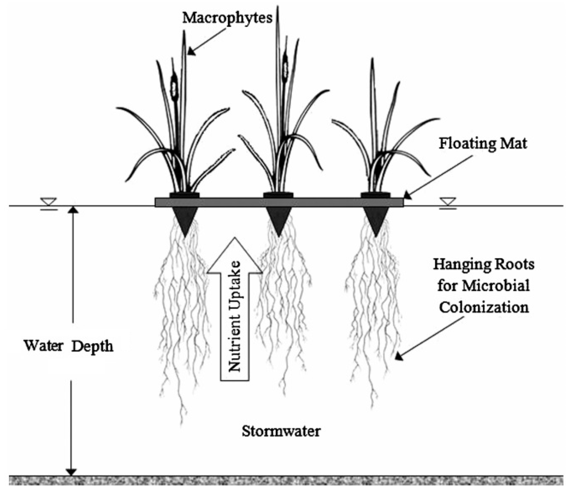
Increases in urban and agricultural development cause stormwater runoffs that contains nutrients that can have severe effects on aquatic ecosystems and human health [1]. The use of floating treatment wetlands (FTWs) is a new and innovative tool to remove nutrients in stormwater wet detention ponds [2]. FTWs represent a human-made ecosystem similar to natural wetlands [3]. A typical FTW is shown in Figure 1 [4].
Vegetation patches or layers are essential in aquatic environments in submerged, emergent, or suspended forms. Suspended canopies, which are the focus of this study, form on the water surface, with stems toward the bottom that do not touch the bottom, in contrast to submerged and emerged canopies that are attached to the bottom. Lemnaceae, Eich- hornia crassipes, Pistia stratiotes, Salvinia molesta, and Laminariales are typical examples of suspended canopies [5,6,7]. Lemnaceae are used extensively for the purpose of purifying wastewater and eutrophic water bodies [8]. Suspended canopies in flow have been investigated in terms of the ecological effects [9,10,11,12] and the mean velocity and turbulence structures of open-channel flows included in these types of canopies [6,7]. Fishing activities and marine navigation can be at risk because of these types of floating vegetation patches [8]. Bed friction has a substantial effect on the velocity and turbulence below and within floating vegetation patches [6,13], however, it has a small role on the flow structure inside submerged or emergent canopies [14,15,16,17,18,19,20,21]. Despite the increasing importance of suspended canopies, there is still a limited number of studies on them. Detailed flow structures in the wake regions of the suspended canopies should be examined to understand the transport of fluid and pollutants.
Liu et al. [22] studied longitudinal dispersion in flow along the floating vegetation patch. They also indicated that a large number of studies on the longitudinal dispersion in open-channel flows with submerged and emergent vegetation have been presented [16,23,24,25]. However, there is an insufficient number of studies on the effects of floating vegetation patches in the literature [22]. They proposed a four-zone model with which they defined the velocity profile and turbulent diffusion coefficient profile for the four zones in their study.
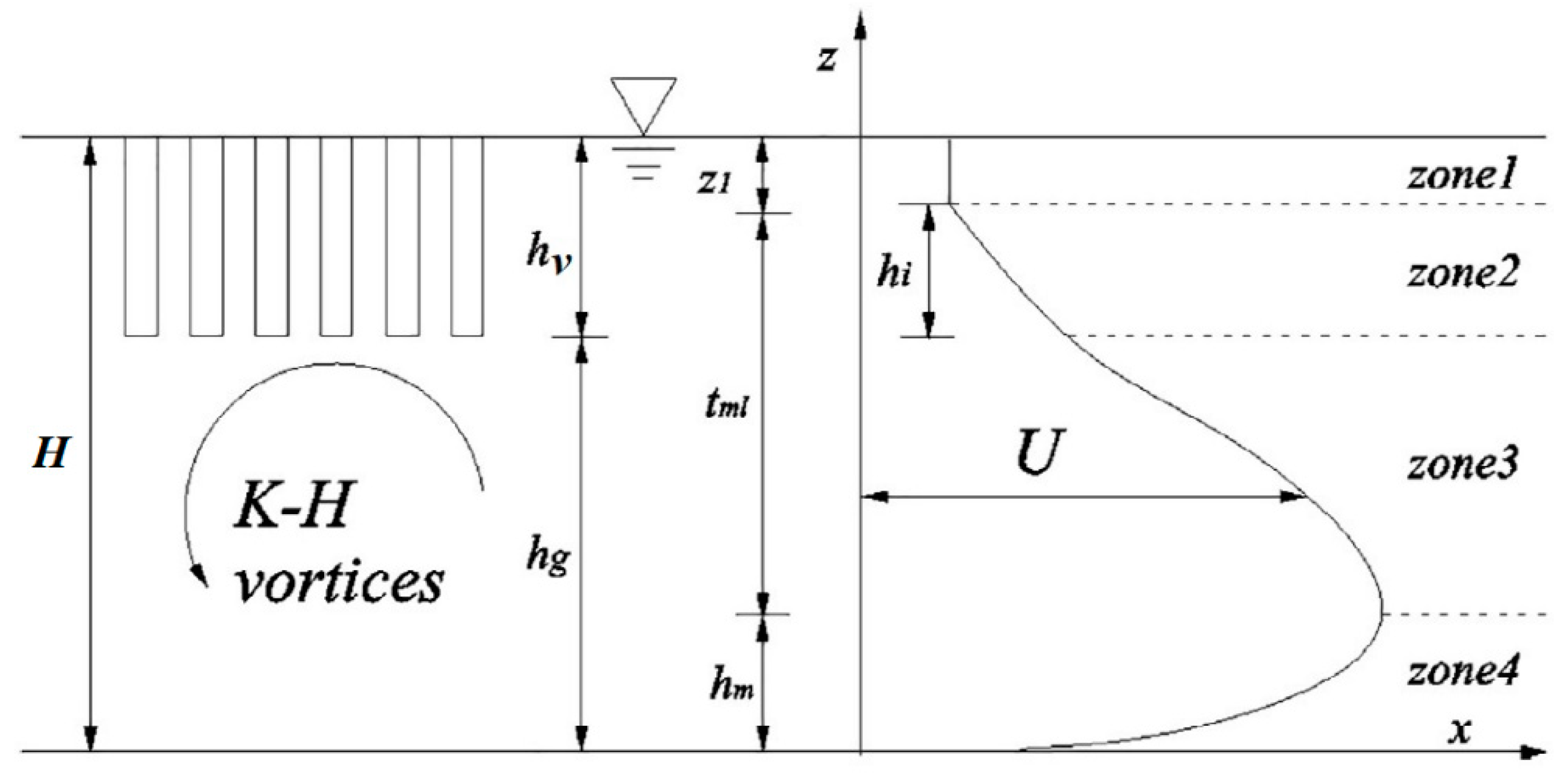
Huai et al. [7] studied the effect of suspended vegetation on velocity distribution at open-channel flows. They considered four different submergence ratios (hv/H = 0.125–0.5, where hv is submergence ratio of the suspended vegetation and H is the flow depth) with a constant density (defined as the canopy projected area per unit volume, a = 1.272 m−1) of the canopy in their experiments. They defined four parts along the flow depth with the suspended vegetation (Figure 2) and determined the velocity profile for every part with the solution of the momentum equation. They called Zone 1 and Zone 2 the outer and internal vegetation layers, respectively. They explained that the drag force of vegetation is dominant in Zone 1 where the velocity is slow and almost constant. The velocity in this zone corresponds to that of the wake region in the submerged vegetated flow [7]. They defined the non-vegetated layer with two zones: Zone 3 and Zone 4. Kelvin–Helmholtz (K–H) vortices characterize the middle mixing layer (tml), which is placed near the bottom of the suspended vegetation [22]. The K–H vortices control the vertical mass transport in the lower region of the suspended vegetation and in the upper part of the gap, which is the non-vegetated region of the flow [26,27]. Zone 2 corresponds to the penetration depth, hi, where the length of the K–H vortices penetrate the vegetation region [22]. The non-vegetated area in the mixing layer is defined as Zone 3, in which the thickness is tml−hi [22]. The resistance caused by suspended vegetation affects Zone 1, Zone 2, and Zone 3, while the friction resistance of the bed affects Zone 4, as it is located close to the bed [22]. The velocity has a maximum value at the junction of Zones 3 and 4. Liu et.al. [22] stated that because of the maximum velocity, the Reynolds shear stress has zero value at this point where the impacts of river bed and suspended vegetation are consistent.
The wake structure downstream of a circular suspended porous obstruction, which represents a model of a suspended vegetation patch, was investigated in this paper. The main question of this study is how the submergence ratio affects the structure of the wake and flow close to the bed, downstream of the suspended patch. For this purpose, the velocity measurements were performed along with the flow depth downstream of the canopy for different submergence ratios with different patch porosities.
2. Experimental Methods
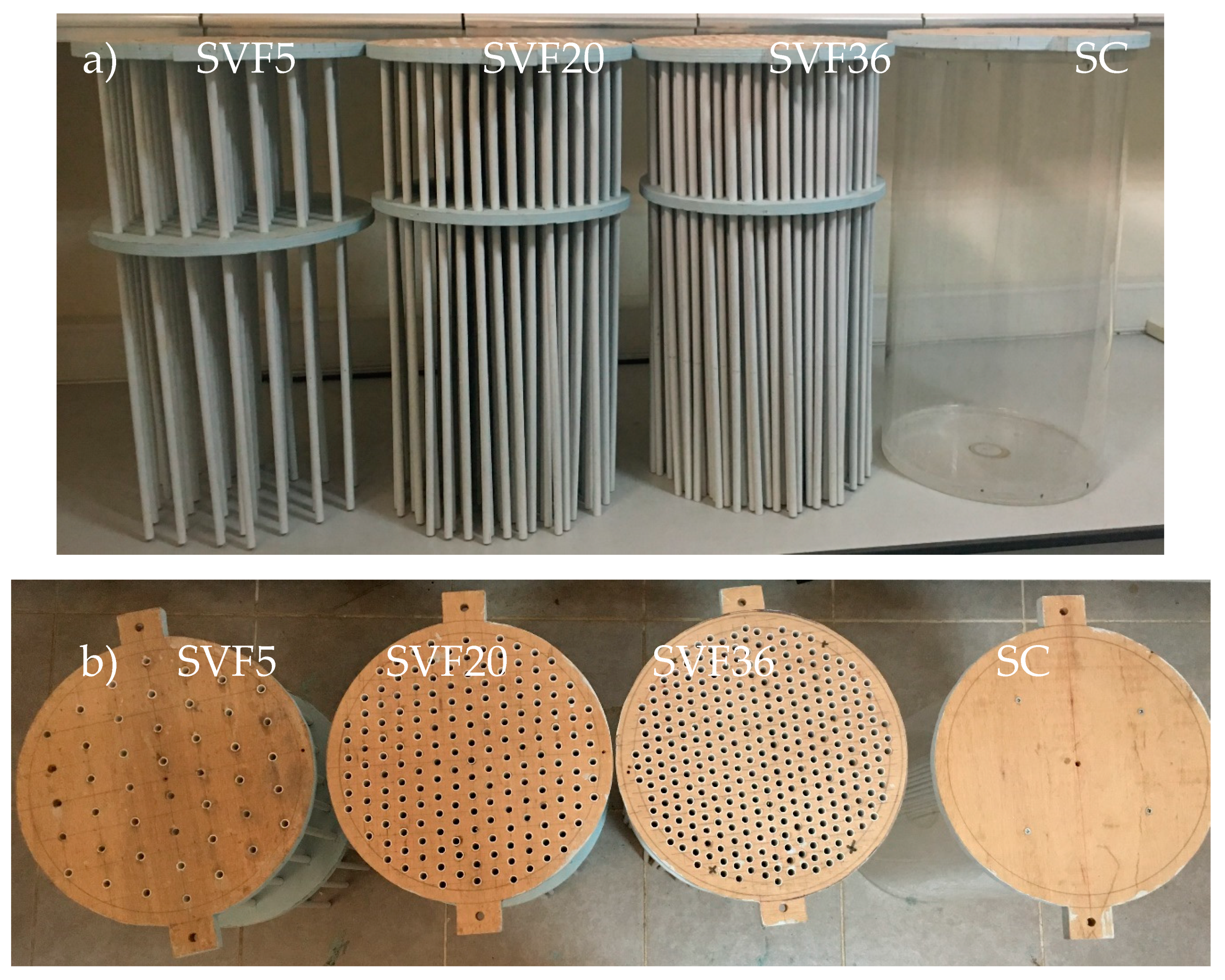
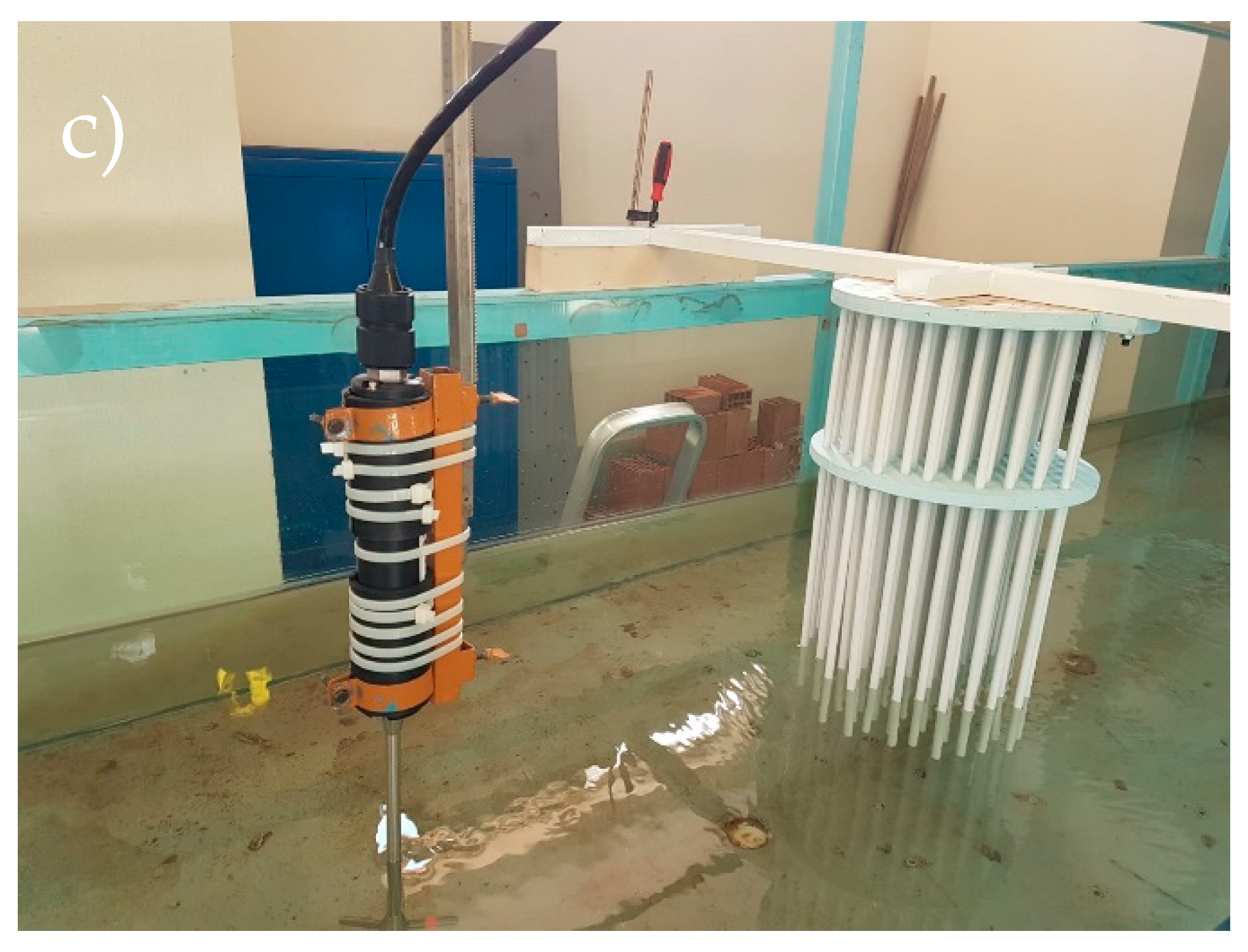
Experiments were performed in an 11 m long, 1.2 m wide, and 0.75 m deep re-circulating glass flume with a concrete horizontal bed at the Civil Engineering Laboratory of Aydın Adnan Menderes University (Figure 3). The suspended vegetation patch was of diameter D = 0.3 m and was formed by rigid plastic cylinders of diameter d = 0.01 m (Figure 4). The cylinders were arrayed in a staggered pattern (Figure 5). The suspended patch was placed at the center of the flume in the transverse direction. The number of cylinders per unit bed area, n (IP/cm2), defines the density of the patch. Here, IP means individual plant number per square centimeter and area is the A = πD2/4. Vegetation density is defined as the frontal area per unit volume, given with a = nd (cm−1), and characterizes the blockage caused by the vegetation layer [28]. The average solid volume fraction is defined with ϕ = nπd2/4 ≈ ad [29]. In the experiments, three different densities of the canopy patch and a solid cylinder were used to simulate the suspended vegetation (Table 1). The Plexiglas solid cylinder was composed as a closed cylinder with D = 30 cm to represent the suspended Solid Case (SC) in the flow area (Table 1). Additionally, a constant mean depth-averaged velocity (Udm = 0.116 m/s) and constant flow depth (H = 0.3 m) were considered in the experiments. Here, velocity values were integrated along the flow depth to calculate mean depth-averaged velocity (Udm). Mean depth-averaged velocity (Udm) was used to calculate Reynolds number and Froude Number for the non-vegetated case. Here, g is the gravitational acceleration, and ν is the kinematic viscosity. Patches were immersed in the flow at two different heights: hv1 = 0.1 m and hv2 = 0.2 m. The cases at the experiments are outlined in Table 1.
In this study, x, y, and z are the longitudinal, transverse, and vertical coordinates, respectively. The origin of the coordinate system is at the upstream edge of the suspended vegetation for the x–y plane and the flume bed for the z direction (Figure 6). A 3-D Acoustic Doppler Velocimeter (ADV) SonTek 10 MHz with a 3-D down-looking probe was used to measure three instantaneous components of velocity (u, v, w), corresponding to x, y, and z directions shown in Figure 6, respectively, during 120 s at 25 Hz. The velocity range was ±0.30 m/s, with a measured velocity accuracy of ±0.5%, and the sampling volume diameter was 6 mm established 0.05 m down from the probe in the experiments. The velocity measurements were conducted at 11 points in the x-direction and at eight different levels along the flow depth (Figure 6). Measurement points along the x-direction were chosen by moving at intervals of 15 or 30 cm upstream and downstream of the vegetation patch (Figure 6c). Alongside this, measurement points along the Z direction were placed at different intervals which correspond to Z1 = 0.5 cm, Z2 = 1.0 cm, Z3 = 1.5 cm, Z4 = 2.0 cm, Z5 = 3.0 cm, Z6 = 4.5 cm, Z7 = 6.0 cm, Z8 = 8.0 cm, Z9 = 11.0 cm, and Z 10 = 15.0 cm (Figure 6a,b). The ADV company suggests that a 15 db signal-to-noise ratio (SNR) and a correlation coefficient larger than 70% for high-resolution measurements [30]. For this reason, conditions where SNR <15 db and the correlation coefficient <70% are used to remove the low-quality samples in the measured data.
3. Results and Discussion
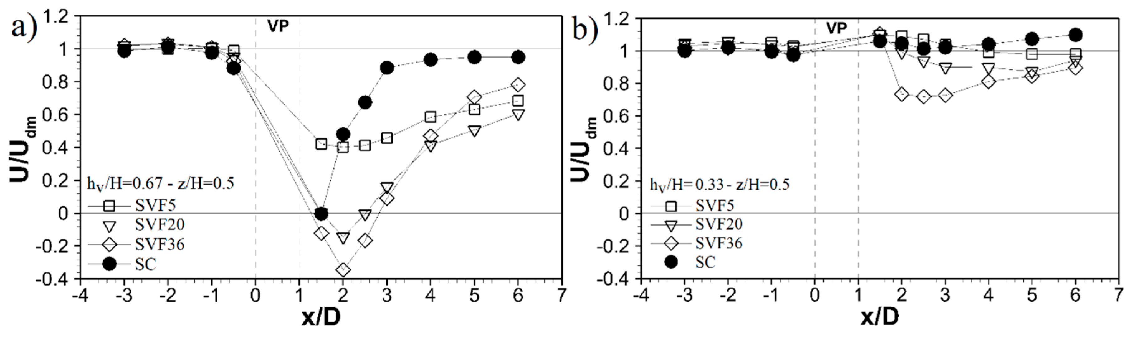
The longitudinal profiles of streamwise averaged velocity, U, for various different densities of patches at mid-depth (z/H = 0.5), for hv/H = 0.67, and hv/H = 0.33, are presented in Figure 7. Here, the vegetated part (VP) corresponds to the suspended vegetation canopy and the mid-depth corresponds to beneath the patch for hv/H = 0.33. The diversion of flow begins almost one diameter upstream of the patch, which is consistent with Rominger and Nepf’s [31] results (Figure 7a). There is a recirculation zone (U < 0) downstream of the flow, which extends to 1.5 D and 2 D distance from the edge of the patch for SVF20 and SVF36, respectively (Figure 7a). As the density increases, the recirculation zone moves downstream and the magnitude of negative streamwise velocity increases. Moreover, there is no recirculation zone for the lowest density (SVF5). Zong and Nepf [29] found that there is a recirculation region in the wakes behind denser patches (ϕ = 0.10), but absent in the wakes of sparser patches (ϕ = 0.03). This result is consistent with our results. A steady wake region was observed downstream of the patch, close to the patch for SVF5, which is not present at higher SVFs in this study. Here, steady wake corresponds to 2 D distance beyond the end of the patch, where U velocity is almost constant.
Zong and Nepf [29] mentioned that the wake can never perfectly recover since the drag-induced momentum deficit should be constant downstream of the obstruction. They further pointed out that the total length of the wake, L, is defined as the distance from the downstream end of the patch to a point where the velocity recovery rate is induced to . The total length of the wake (L) is almost 3 D at mid-depth for the solid body and for ReD = 3.5 × 10⁴ (Figure 7a). This value is consistent with Zong and Nepf’s [29] results, in which L = 3 D and L = 3.3 D for ReD = 2.2 × 10⁴ and ReD = 4.1 × 10⁴, respectively, in their study. Cantwell and Coles [32] also defined L = 2.5 D for a cylinder wake at ReD = 1.4 × 10⁵ in their study. The recovery region extends to 5 D beyond the end of the patch in our study. Another noteworthy situation is that U increases rapidly to Udm at the highest density (SVF36) compared to the lower densities (SVF5 and SVF20) (Figure 7a).
Considering the lower depth ratio (h/H = 0.33), there is almost no effect of the patch beneath the patch at mid-depth for the solid body and lowest SVF (Figure 7b). However, suspended vegetation still affects the flow beneath the patch for a higher density of patches (SVF20 and SVF36). The obstruction effect on the flow is higher at the highest patch density (SVF36).
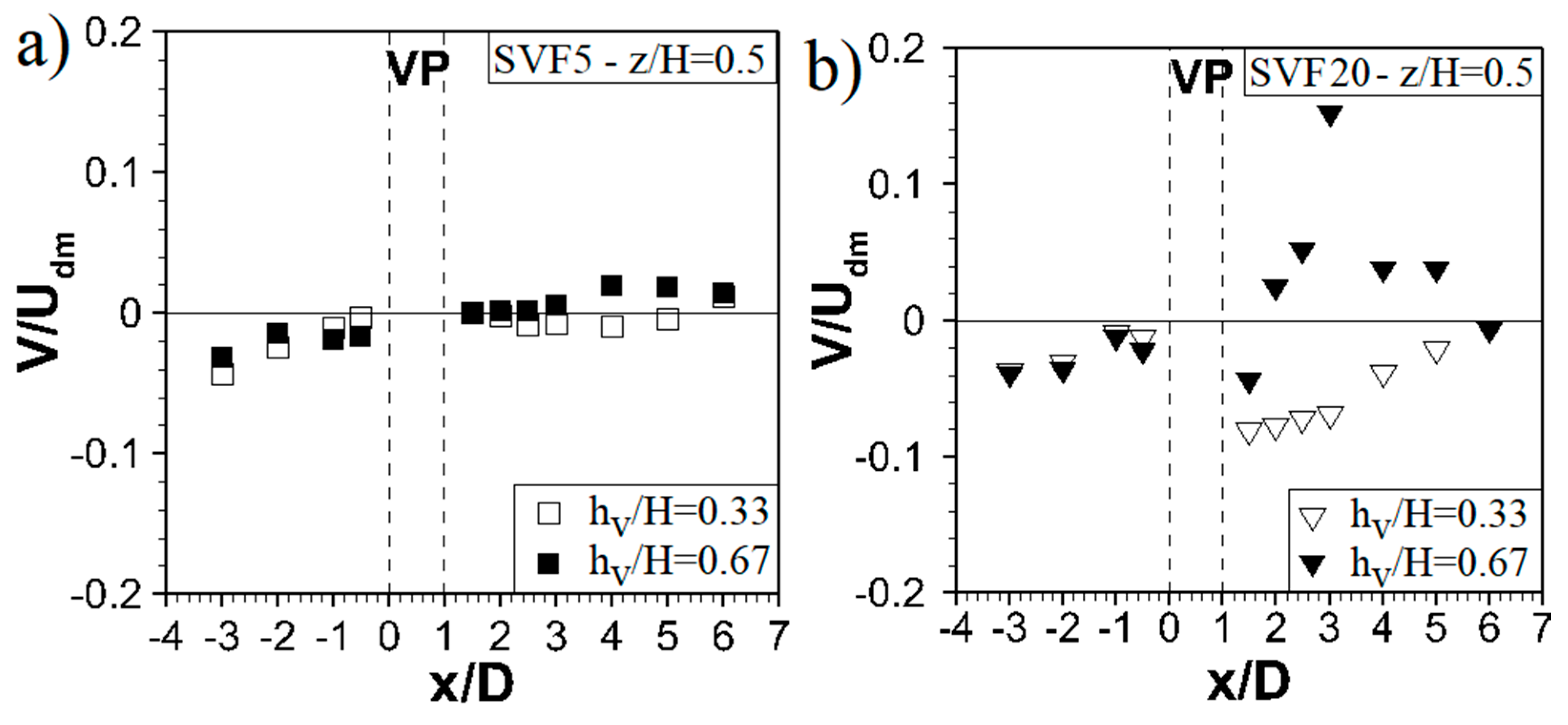
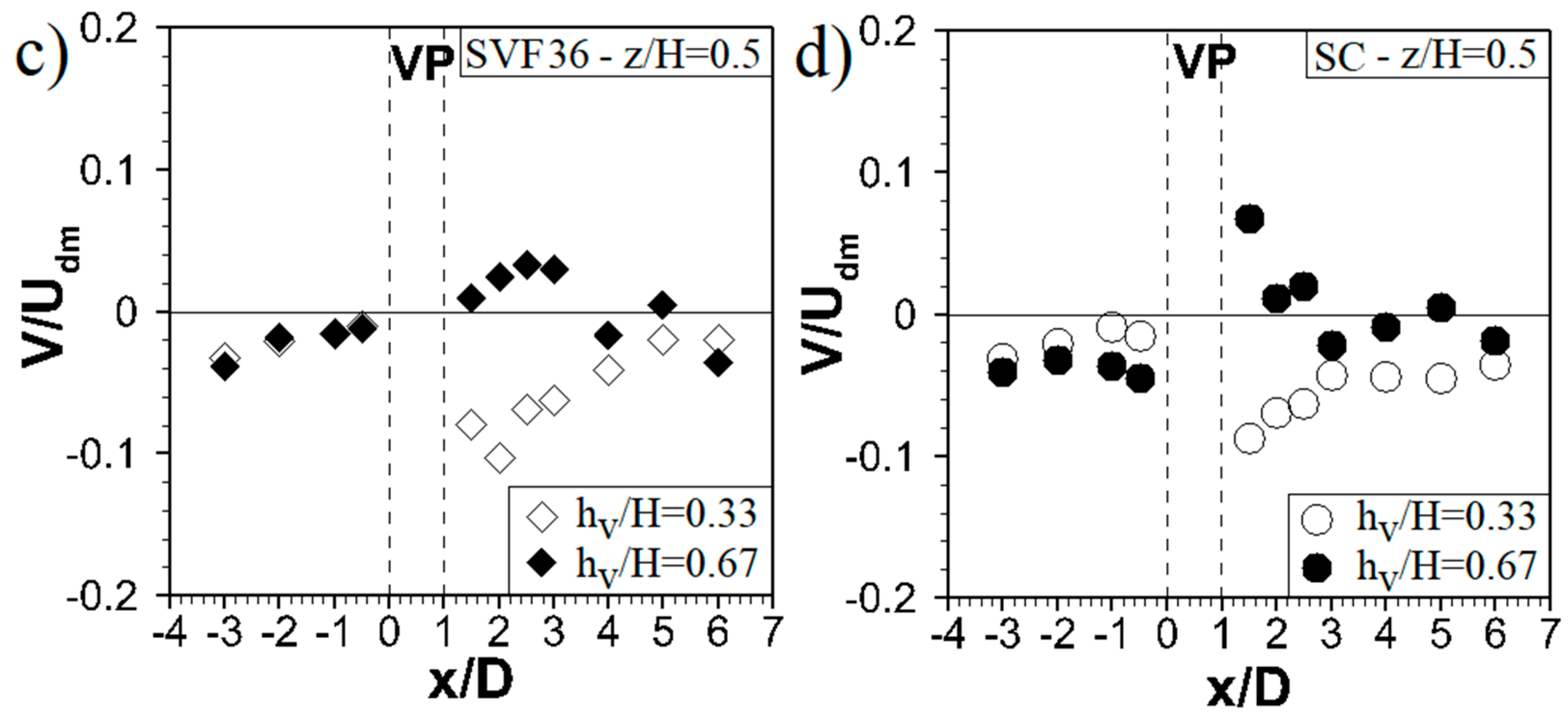
Longitudinal profiles of time-averaged transversal velocity, V, for different densities of patches and depth ratios at mid-depth were also examined (Figure 8). A suspended vegetation patch does not have a significant effect on transversal velocity beneath the patch for a low solid volume fraction (SVF5) at a lower depth ratio (hv/H = 0.33) (Figure 8a). As the suspended canopy become denser, the magnitude of the transversal velocity increases downstream until 2 D distance from the end of the patch for a lower depth ratio (hv/H = 0.33). Similar to a lower depth ratio, there is almost no effect on transversal velocity downstream of the patch for low solid volume fractions at higher depth ratios (hv/H = 0.67) (Figure 8a). There is diverging flow downstream of the patch which extends until 5 D distance for SVF20, 3 D distance for SVF36, and 1 D distance for the Solid Case. The position of diverging flow occurs closer to the patch with the increasing SVF. Transversal velocity varies around zero beyond the point where the diverging of the flow ends.
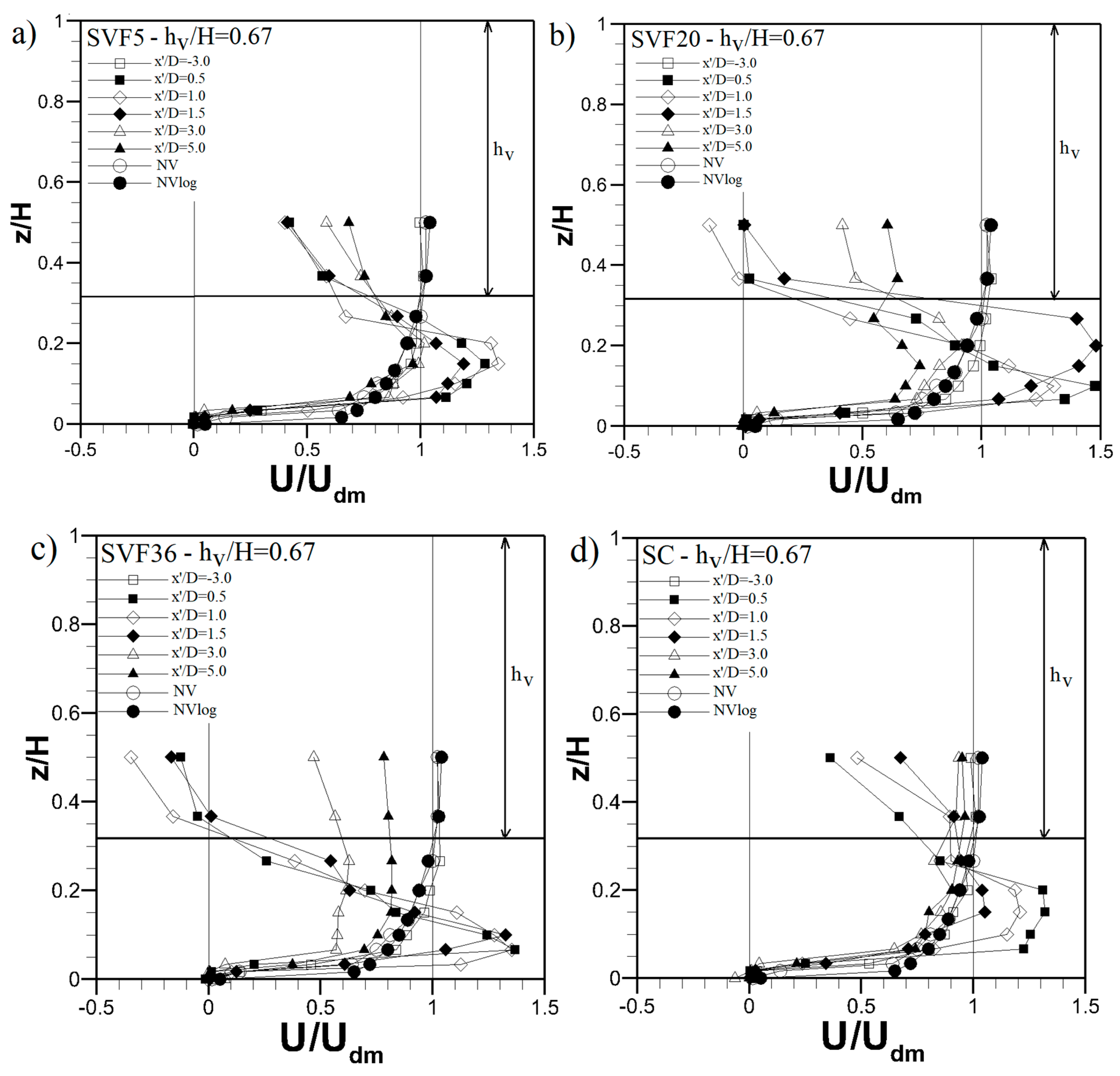
Figure 9 shows the vertical profiles of the normalized velocity U/Udm at different upstream and downstream positions (x’/D) for hv/H = 0.67. Here, x’ refers to the distance from the patch edge and NV and NVlog correspond to the normalized velocity (U/Udm) distribution and normalized logarithmic velocity (Ulog/Udm) distribution, respectively, at non-vegetated flow conditions. You can find detailed information about the calculation of Ulog from Yılmazer et al. [17]. A combination of a channel bed and suspended patch causes maximum velocity at the gap, with a flow similar to a wall jet beneath the vegetation patch. Here, the layer between the bed and the maximum velocity point is called the inner layer, where wall shear is effective; the area above the point of the maximum velocity is called the outer layer, where patch shear is effective. Flow has a maximum velocity of almost 1.45–1.5 Udm beneath the patch and downstream for higher densities of patches (SVF20 and SVF36). Comparatively, the maximum velocity for the lowest density of patches (SVF5) is around 1.3 Udm, which is similar to the Solid Case. It can be concluded that there is a suspended patch effect that increases the velocity beneath the suspended patch for a certain range of SVF, which corresponds to high densities of patches. Another important point is the placing of the maximum velocity, which is z/H ≅ 0.15 for SVF20 and SVF36, and z/H ≅ 0.3 for SVF5 and the Solid Case. Inner layer thickness decreases with the increasing SVFs. The placement and the magnitude of the maximum velocity at the gap region shows similar behavior at SVF5 and the Solid Cases, which is similar for higher densities (SVF20 and SVF36). It can be concluded that the individual patch elements have an important role for lower densities, which is SVF5 in this study. U velocity has negative values downstream of the patch for the densities SVF20 and SVF36, and its value increases with increasing patch density at the near-wake region (~x’/D ≤ 1.5 D). There is no reversed flow region for the lowest density patch (SVF5) and solid patch. Moreover, the flow behavior at the Solid Case is similar to the lower densities of the patch, e.g., SVF5. Maximum velocity value bigger than Udm is present along x’ < 3 D, downstream of the gap region, which also corresponds to the distance where flow behavior is similar to wall jet flow.
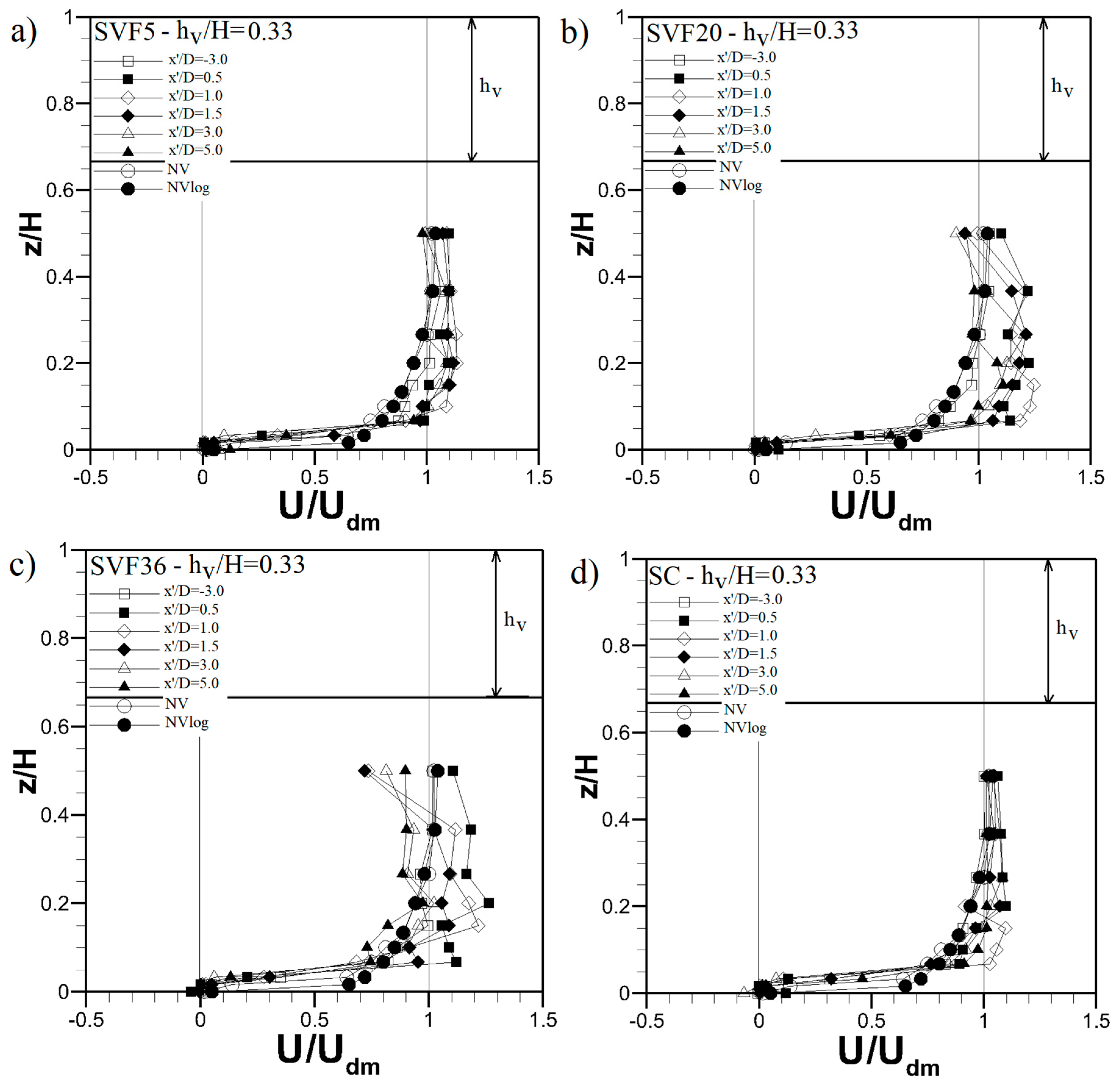
The vertical profiles of U velocity for different densities of patches are shown in Figure 10 for hv/H = 0.33. Velocity distribution and flow behavior deviate at x’ = 0.5 D distance downstream of the patch, and is totally different in the case of a higher submergence ratio. The patch does not have a big effect on the flow structure along with the entire flow depth for this submergence ratio. The behavior of the velocity distribution for SVF20 and SVF36 is similar, as is the case for SVF5 and the solid patch. Flow has a maximum velocity of almost ~1.25 Udm for higher densities (SVF20 and SVF36) and around ~1.1 Udm for the lowest density (SVF5) and Solid Case. This result shows us that it is still possible to see the effect of density for high densities (SVF20 and SVF36 in this study) downstream of the gap region for lower submergence ratios. Downstream of the gap region, a maximum velocity value bigger than Udm is present along x’ < 3 D for SVF36 and SC, and x’ < 5 D for SVF5 and SVF20. It can be concluded that a high density of the submerged vegetation patches still has an influence on the flow structure beneath the patch, even at low submergence ratios.
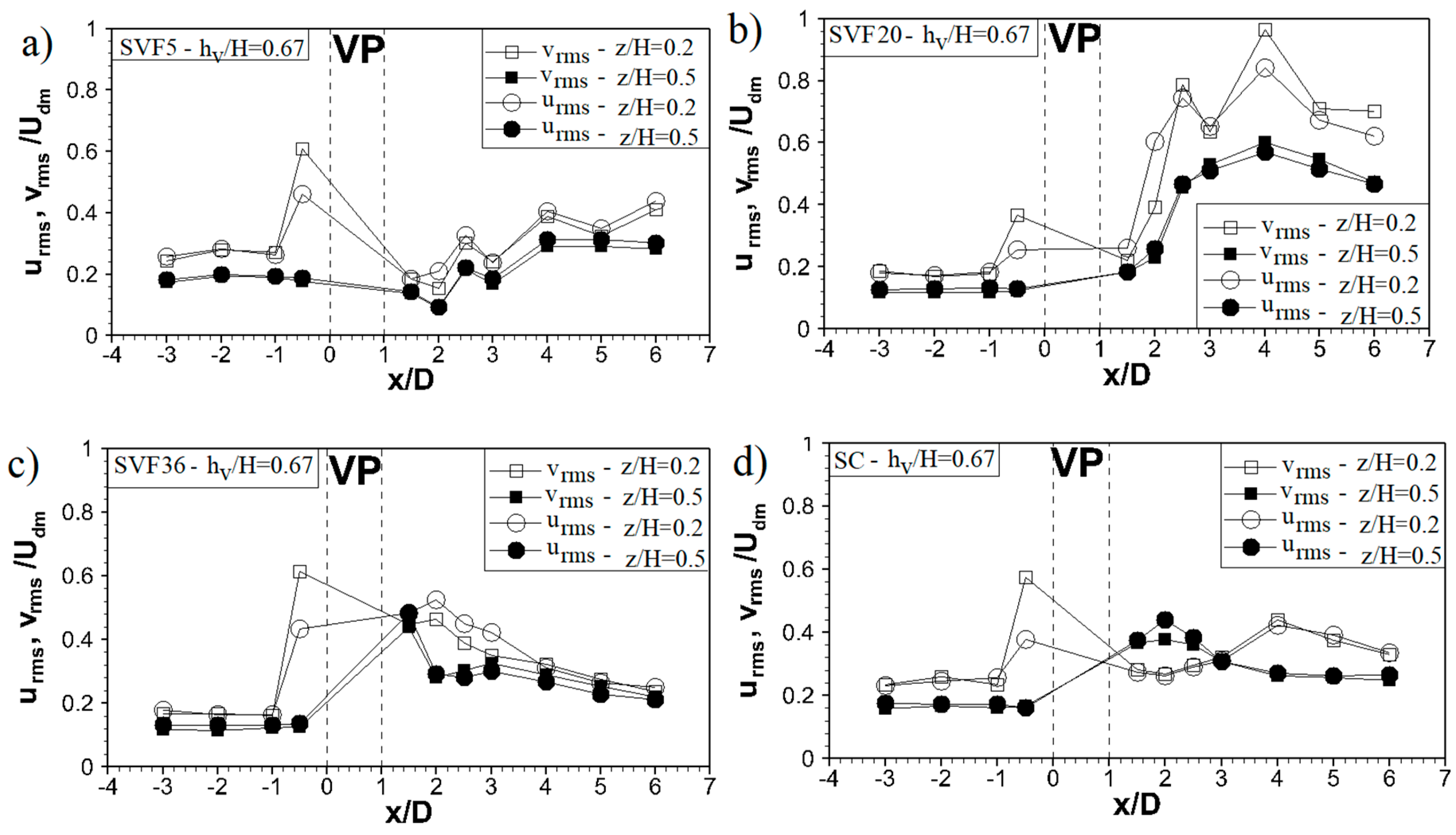
Longitudinal profiles of and for different densities of patches at different depths (z/H = 0.2 and z/H = 0.5) along the streamwise direction for hv/H = 0.67 are shown in Figure 11. Here, z/H = 0.2 corresponds to the gap region and z/H = 0.5 corresponds to the upstream and downstream parts of the patch. First of all, velocity fluctuations are higher upstream of the gap region than upstream of the patch for all cases. Moreover, there is a peak at x’= –0.5 D upstream of the gap region that is not present upstream of the patch. This shows us that the effect of a submerged obstruction starts in the upstream section, below the obstruction. Turbulence starts with a decaying trend downstream, and then it starts to increase for SVF5 and SVF20 cases at both levels. Specifically, the shear layer caused by the patch increases the turbulence level beneath the patch. Turbulence shows a decaying trend for SVF36, which is the highest density of patches, and the values of turbulence become closer at x’ = 3 D distance for different depths (z/H = 0.2 and z/H = 0.5). This shows us that the individual stem turbulence is not significant for the highest patch density (SVF36), but is significant at lower patch densities (SVF5 and SVF20). Individual cylinders cause small-scale turbulence, which results in a higher turbulence region behind the patch. The turbulence level has the highest value, especially for SVF20, in the near-wake region of the patch in this study. This is because of the significance of the individual cylinders for the patch intensity.
Comparing the cases of SVF20 and SVF36, the turbulence level decreases with increasing patch density (SVF36) to a level close to that of the solid body at mid-depth. This shows that the suspended patch with the highest porosity patch (SVF36) behaves like a solid body. The turbulence level is higher downstream of the solid body than it is downstream of the gap region along x’ = 2 D distance, beyond which point it is reversed (Figure 11d). After this point, the magnitude of the turbulence is similar for the highest density (SVF36) of patches and the solid body at mid-depth. However, the magnitude of the turbulence is higher for the solid body than the highest density (SVF36) of patches in the recovery region. This may occur because of the wake region behind the solid body. There is only one point, which is the closest point to the patch, (x = 0.5 D) downstream of the highest density patch (SVF36), where turbulence is higher than the solid body at mid-depth. This point corresponds to the wake region of the individual stem of the highest density patch. This shows us that the highest density patches behave like a solid body at the wake region, with the exception of very close to the patch (x ≤ 0.5D).
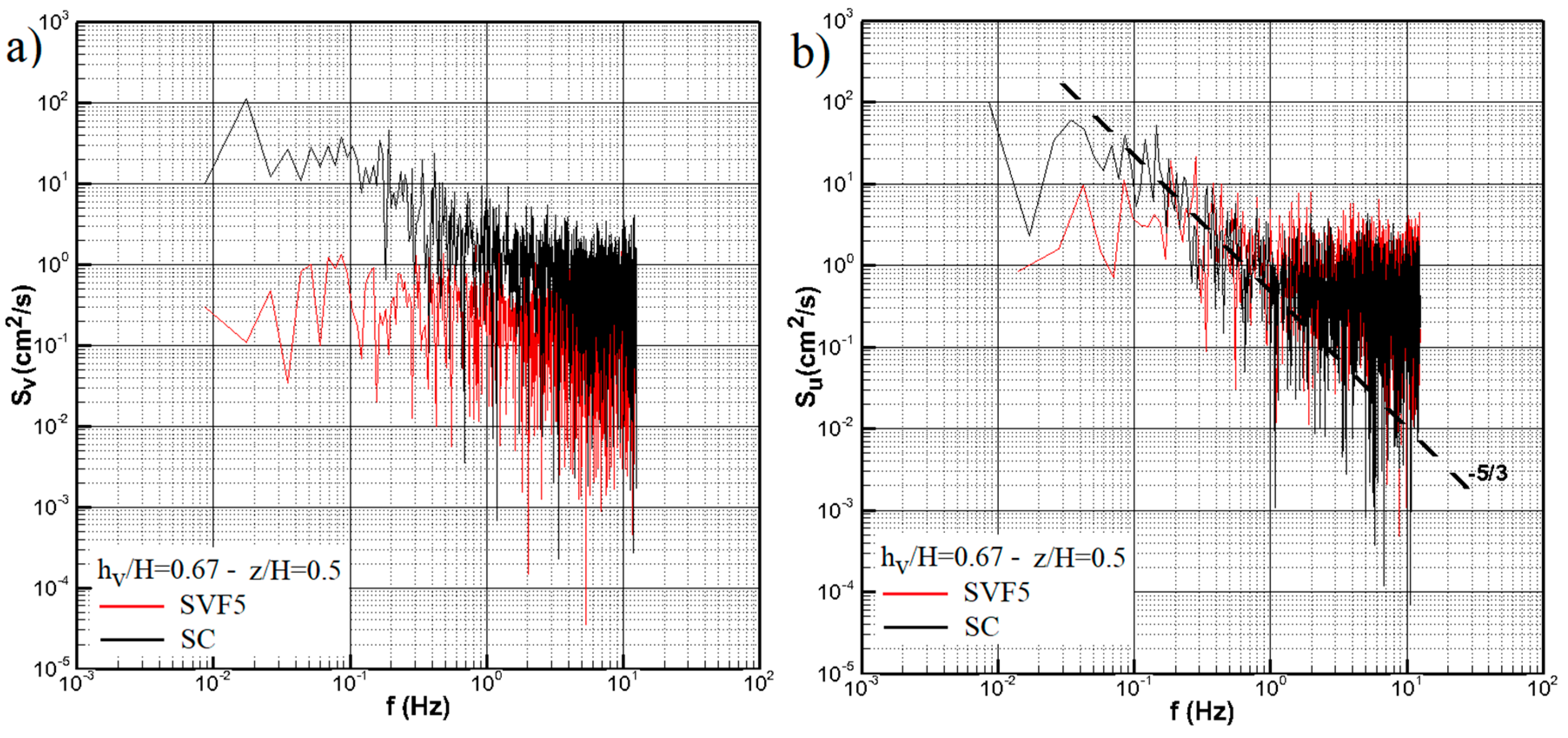
Figure 12a shows the spectral density variation of transverse velocity with frequency for Case SVF5 and the Solid Case. The eddy dominant frequency corresponds to the peak velocity spectra Svvpeak. Case SVF5 and the Solid Case are discussed as representative examples and for the comparison of the canopy and Solid Cases (Figure 12). The dimensionless Strouhal number (St = fL/Udm) defines the relationship between the characteristic length of a vortex and the frequency. Here, f is the vortex shedding frequency (dominant frequency), L is the characteristic vortex length, and Udm is the characteristic flow velocity. St is almost constant around St = 0.2 within a wide range of Reynolds numbers, between Re = 250 to 2 × 10⁵ for flows passing a cylinder [33]. Zhao and Huai [34] assumed that this can also be used for the bundle of cylinders in their study. Therefore, we considered St = 0.2 for both Case SVF5 and the Solid Case. For Case SVF5 (x’/D = 0.5 and z/H = 0.5), the vortex shedding frequency is f = 0.08 Hz (Figure 12a) and the characteristic velocity Udm is approximately 0.116 m/s. The characteristic vortex length L is almost 0.293 m, which is almost equal to the diameter of the patch (D = 0.3 m). For the Solid Case (x/D = 0.5 and z/H = 0.5), the vortex shedding frequency is f = 0.11 Hz (Figure 12a) and the characteristic velocity Udm is almost 0.116 m/s. The characteristic vortex length L is almost 0.211 m, which is smaller than the canopy diameter. When the magnitude of the peaks in Svv is compared, it is clear that the turbulence intensity of the wake-scale vortices is greater for the solid body than for the patch, which is consistent with Zong and Nepf’s [29] results. This magnitude difference becomes smaller moving further downstream of the patch.
Figure 12b shows the change in longitudinal velocity spectral density with frequency for Case SVF5 and the Solid Case. When the frequency exceeds 0.16 Hz for the Solid Case and 0.04 Hz for SVF5, the linear decrease of spectral densities is in agreement with the Kolmogorov line, with a slope of −5/3, as shown in Figure 12b.
Channel blockage D/B = 0.25 (Figure 3) in this study may have some effect on the vortex shedding frequency in our study. Chen et al. [35] and Coutanceau and Bouard [36] stated that both Rec and the Strouhal number (StD = fD/Udm) increase with increasing channel blockage. Here, Rec is the critical Reynolds number at which unbounded steady flow past a circular cylinder becomes unstable. Sahin and Owens [37] found that Rec and StD were 285 and 0.44, respectively, for a blockage of 0.64. Zong and Nepf [29] considered D/B = 0.10, 0.18, and 0.35 for the emergent patch in their study and showed that ReD (=UdmD/ν) is O (104), which is within the turbulent wake regime. In our study, ReD is O (105), which is the within the turbulent wake regime. As a result, the channel blockage might have some effects on the vortex shedding frequency in our study.
Rominger and Nepf [31] defined deceleration through a long porous patch where length is much larger than width. They mentioned that the velocity at the centerline starts to decline from some distance upstream of the patch, which was also observed in this study (Figure 7a), and that the deceleration continues into the patch over a length xD, after which the flow reaches a steady velocity, U0—the final interior velocity. Rominger and Nepf [31] obtained that the interior adjustment length (xD) and the final interior velocity (U0) depend on the dimensionless parameter, , which is called the patch flow-blockage. Here, CD is the drag coefficient for the cylinders within the patch.
A low blockage effect is present for , where interior velocity is driven by turbulent stress; while in a high blockage effect, when , interior velocity is driven by a pressure gradient [29,31]. In our study, for ϕ = 0.05 (SVF5), for ϕ = 0.20 (SVF20), and for ϕ = 0.36 (SVF36), where CD = 1 for simplicity, as Zong and Nepf [29] considered in their study. There is a low blockage regime for the case ϕ = 0.05 < 0.1 and at this regime xD ~ 2 (CDa)−1 [31] and xD = 33.33 cm in this study. Here, CDa is the canopy drag length scale, which is the length scale of flow deceleration associated with canopy drag. There is high blockage regime for the cases ϕ = 0.20 > 0.1 and ϕ = 0.36 > 0.1, which is consistent with Zong and Nepf’s [29] experimental conditions. In these cases, the interior adjustment length xD ~D = 30 cm and diameter of the canopy patch provide us this length. As such, velocity just downstream of the patch is expected to be equal to the interior velocity for these cases.
4. Conclusions
The purpose of this study was to answer how the submergence ratio and density of vegetation patches affects the flow structure along the axis of the patch, downstream of the suspended cylindrical vegetation patch. For this purpose, the velocity measurements with ADV (Acoustic Doppler Velocimeter) were performed along the flow depth at the axis of the patch along different longitudinal distances downstream of the suspended patch for different submergence ratios (hv1/H = −0.33 and hv2/H = 0.67) and different patch porosities (ϕ1 = 0.05, SVF5; ϕ2 = 0.20, SVF20; ϕ3 = 0.36, SVF36; ϕ4 = 1.00, Solid Case).
It was found that there is a recirculation zone behind the obstruction, which is strongest for the highest density (SVF36) patch, while there is no recirculation zone for the lowest density (SVF5). It was also shown that U velocity increases more rapidly to the Udm value at the highest density (SVF36) compared to the lower densities (SVF5 and SVF20). Moreover, a steady wake region was observed downstream of the patch for SVF5, which is not present at higher SVFs.
The flow becomes stronger downstream of the gap region with increasing submergence ratio and flow behavior becomes similar to wall jet flow. It was found that SVF has an important impact on this flow structure in terms of the magnitude and the placement of the maximum velocity.
The patch with the lower depth ratio (hv/H = 0.33) affected the flow slightly downstream for the solid body and lowest SVF. However, suspended vegetation still affects the flow downstream of the gap region for a higher density of patches (SVF20 and SVF36) and it is concluded that high densities of submerged vegetation patches still have an influence on the flow structure downstream of the gap, even at low submergence ratios.
It was found that suspended vegetation patches do not have a significant effect on transversal velocity downstream of the patch for a low solid volume fraction (SVF5) at both depth ratios. As the suspended canopy becomes denser, the magnitude of transversal velocity increases, and the placement of diverging flow occurs closer to the patch, in the downstream section, with increasing SVF.
The effect of suspended vegetation on turbulence starts in the upstream section and causes a peak upstream of the gap region. It was found that the shear layer caused by the patch increases the turbulence level beneath the patch. It was also found that the individual stem turbulence is not significant for the highest patch density (SVF36), whereas it is significant at lower patch densities (SVF5 and SVF20). Individual cylinders cause the small-scale turbulence, which results in a higher turbulence region behind the patch. Moreover, the turbulence level decreases with increasing patch density (SVF36) and this turbulence level is close to the turbulence level for the solid body at mid-depth. This means that the suspended patch with the highest porosity patch (SVF36) behaves like a solid body in terms of turbulence and structure of the flow.
Author Contributions
A.Y.O. and D.Y. conceived and designed the experiments; A.Y.O. and D.Y. performed the experiments; A.Y.O. and D.Y. analyzed the data; A.Y.O. wrote the paper. All authors have read and agreed to the published version of the manuscript.
Funding
This research received no external funding.
Acknowledgments
The authors would like to thank Aydın Adnan Menderes University, Civil Engineering Department students Omer Botan YILDIZHAN, Ali CAMBOLAT and Ebru ERSIN who helped during the experiments.
Conflicts of Interest
The authors declare no conflict of interest.
References
- Anderson, D.M.; Glibert, P.M.; Burkholder, J.M. Harmful algal blooms and eutrophication: Nutrient sources, composition, and consequences. Estuaries 2002, 25, 704–726. [Google Scholar] [CrossRef]
- Hartshorn, N.; Marimon, Z.; Xuan, Z.M.; Chang, N.B.; Wanielista, M.P. Effect of floating treatment wetlands on control of nutrients in three stormwater wet detention ponds. J. Hydraul. Eng. 2016, 21, 8. [Google Scholar] [CrossRef]
- Sample, D.J.; Laurie, J.F. Innovative Best Management Fact Sheet No. 1: Floating Treatment Wetlands. Available online: https://vtechworks.lib.vt.edu/bitstream/handle/10919/70627/BSE-76.pdf?sequence=1&isAllowed=y (accessed on 19 November 2019).
- Wanielista, M.P.; Chang, N.B.; Chopra, M.; Xuan, Z.; Islam, K.; Marimon, Z. Floating Wetland Systems for Nutrient Removal in Stormwater Ponds; Final Report FDOT Project BDK78 985-01; 2012. Available online: http://frogenvironmental.co.uk/wp-content/uploads/2014/09/Wanielista-et-al-2012-FTW-for-nutrient-removal-in-stormwater-ponds-final-report.pdf (accessed on 19 November 2019).
- Rosman, J.H.; Koseff, J.R.; Monismith, S.G.; Grover, J. A field investigation into the effects of a kelp forest (Macrocystis pyrifera) on coastal hydrodynamics and transport. J. Geophys. Res. 2007, 112, C02016. [Google Scholar] [CrossRef] [Green Version]
- Plew, D.R. Depth-averaged drag coefficient for modeling flow through suspended canopies. J. Hydraul. Eng. 2010, 137, 234–247. [Google Scholar] [CrossRef]
- Huai, W.; Hu, Y.; Zeng, Y.; Han, J. Velocity distribution for open channel flows with suspended vegetation. Adv. Water Resour. 2012, 49, 56–61. [Google Scholar] [CrossRef]
- Zhao, F.; Huai, W.; Li, D. Numerical modeling of open channel flow with suspended canopy. Adv. Water Resour. 2017, 105, 132–143. [Google Scholar] [CrossRef]
- Adams, C.S.; Boar, R.R.; Hubble, D.S. The Dynamics and Ecology of Exotic Tropical Species in Floating Plant mats: Lake Naivasha, Kenya. Hydrobiologia 2002, 488, 115–122. [Google Scholar] [CrossRef]
- Scheffer, M.; Szabo, S.; Gragnani, A. Floating plant dominance as a stable state. Proc. Natl. Acad. Sci. USA 2003, 100, 4040–4045. [Google Scholar] [CrossRef] [Green Version]
- Fang, Y.Y.; Babourina, O.; Rengel, Z. Ammonium and nitrate up-take by the floating plant Landoltia punctate. Ann. Bot. 2007, 99, 365–370. [Google Scholar] [CrossRef] [Green Version]
- Nichols, P.; Lucke, T.; Drapper, D.; Walker, C. Performance Evaluation of a Floating Treatment Wetland in an Urban Catchment. Water 2016, 8, 244. [Google Scholar] [CrossRef] [Green Version]
- Plew, D.R.; Spigel, R.H.; Stevens, C.L.; Nokes, R.I.; Davidson, M.J. Stratified flow interactions with a suspended canopy. Environ. Fluid Mech. 2006, 6, 519–539. [Google Scholar] [CrossRef]
- Nepf, H.M.; Mugnier, C.G.; Zavistoski, R.A. The effects of vegetation on longitudinal dispersion. Estuar. Coast. Shelf Sci. 1997, 44, 675–684. [Google Scholar] [CrossRef]
- Ghisalberti, M.; Nepf, H.M. The limited growth of vegetated shear layers. Water Resour. Res. 2004, 40, W07502. [Google Scholar] [CrossRef]
- Lightbody, A.F.; Nepf, H.M. Prediction of velocity profiles and longitudinal dispersion in salt marsh vegetation. Limnol. Oceanogr. 2006, 51, 218–228. [Google Scholar] [CrossRef]
- Yılmazer, D.; Ozan, A.Y.; Cihan, K. Flow Characteristics in the Wake Region of a Finite-Length Vegetation Patch in a Partly Vegetated Channel. Water 2018, 10, 459. [Google Scholar] [CrossRef] [Green Version]
- Ben Meftah, M.; Mossa, M. Prediction of channel flow characteristics through square arrays of emergent cylinders. Phys. Fluids 2013, 25, 1–21. [Google Scholar] [CrossRef]
- Ben Meftah, M.; De Serio, F.; Mossa, M. Hydrodynamic behavior in the outer shear layer of partly obstructed open channels. Phys. Fluids 2014, 26, 1–19. [Google Scholar] [CrossRef]
- Ben Meftah, M.; Mossa, M. Partially obstructed channel: Contraction ratio effect on the flow hydrodynamic structure and prediction of the transversal mean velocity profile. J. Hydrol. 2016, 542, 87–100. [Google Scholar] [CrossRef]
- Ben Meftah, M.; De Serio, F.; Malcangio, D.; Mossa, M.; Petrillo, A.F. A modified log-law of flow velocity distribution in partly obstructed open channels. Environ. Fluid Mech. 2016, 16, 453–479. [Google Scholar] [CrossRef]
- Liu, X.; Huai, W.; Wang, Y.; Yang, Z.; Zhang, J. Evaluation of a random displacement model for predicting longitudinal dispersion in flow through suspended canopies. Ecol. Eng. 2018, 116, 133–142. [Google Scholar] [CrossRef]
- Cheng, N.S. Representative roughness height of submerged vegetation. Water Resour. Res. 2011, 47, 1–18. [Google Scholar] [CrossRef]
- Shucksmith, J.D.; Boxall, J.B.; Guymer, I. Determining longitudinal dispersion coefficients for submerged vegetated flow. Water Resour. Res. 2011, 47, 124–132. [Google Scholar] [CrossRef]
- Liu, Z.; Chen, Y.; Zhu, D.; Hui, E.; Jiang, C. Analytical model for vertical velocity profiles in flows with submerged shrub-like vegetation. Environ. Fluid Mech. 2012, 12, 341–346. [Google Scholar] [CrossRef]
- Stoesser, T.; Salvador, G.P.; Rodi, W.; Diplas, P. Large Eddy Simulation of Turbulent Flow Through Submerged Vegetation. Transp. Porous Media 2009, 78, 347–365. [Google Scholar] [CrossRef]
- Nepf, H.; Ghisalberti, M. Flow and transport in channels with submerged vegetation. Acta Geophys. 2008, 56, 753–777. [Google Scholar] [CrossRef]
- Kaimal, J.; Finnigan, J. Atmospheric Boundary Layer Flows; Oxford University Press: New York, NY, USA, 1994. [Google Scholar]
- Zong, L.; Nepf, H. Vortex development behind a finite porous obstruction in a channel. J. Fluid Mech. 2012, 691, 368–391. [Google Scholar] [CrossRef]
- Wahl, T.L. Analyzing ADV Data Using WinADV. In Proceedings of the Joint Conference on Water Resources Engineering and Water Resources Planning & Management, Minneapolis, MN, USA, 30 July–2 August 2000. [Google Scholar]
- Rominger, J.; Nepf, H. Flow adjustment and interior flow associated with a rectangular porous obstruction. J. Fluid Mech. 2011, 680, 636–659. [Google Scholar] [CrossRef]
- Cantwell, B.; Coles, D. An experimental Study of Entrainment and Transport in the Turbulent Near Wake of a Circular Cylinder. J. Fluid Mech. 1983, 136, 321–374. [Google Scholar] [CrossRef] [Green Version]
- Schlichting, H. Boundary-Layer Theory; McGraw-Hill: New York, NY, USA, 1979. [Google Scholar]
- Zhao, F.; Huai, W. Hydrodynamics of discontinuous rigid submerged vegetation patches in open-channel flow. J. Hydro-Environ. Res. 2016, 12, 148–160. [Google Scholar] [CrossRef]
- Chen, J.H.; Pritchard, W.H.; Tavener, S.J. Bifurcation for flow past a cylinder between parallel planes. J. Fluid Mech. 1995, 284, 23–41. [Google Scholar] [CrossRef]
- Coutanceau, M.; Bouard, R. Experimental determination of the main features of the viscous flow in the wake of a circular cylinder in uniform translation. Part 1. Steady flow. J. Fluid Mech. 1977, 79, 231–256. [Google Scholar] [CrossRef]
- Sahin, M.; Owens, R.G. A numerical investigation of wall effects up to high blockage ratios on two-dimensional flow past a confined circular cylinder. Phys. Fluids 2004, 16, 1305–1320. [Google Scholar] [CrossRef]
Figure 1.
An example of floating treatment wetland [4].
Figure 1.
An example of floating treatment wetland [4].

Figure 2.
Schematic velocity distribution in suspended vegetated flow [22].
Figure 2.
Schematic velocity distribution in suspended vegetated flow [22].

Figure 3.
Experimental set-up: (a) plan view, (b) cross-section (units are in cm).

Figure 4.
Photos from vegetation patches for different SVFs (Solid Volume Fractions): (a) side view, (b) top view, (c) view from an experiment with an Acoustic Doppler Velocimeter (ADV).
Figure 4.
Photos from vegetation patches for different SVFs (Solid Volume Fractions): (a) side view, (b) top view, (c) view from an experiment with an Acoustic Doppler Velocimeter (ADV).


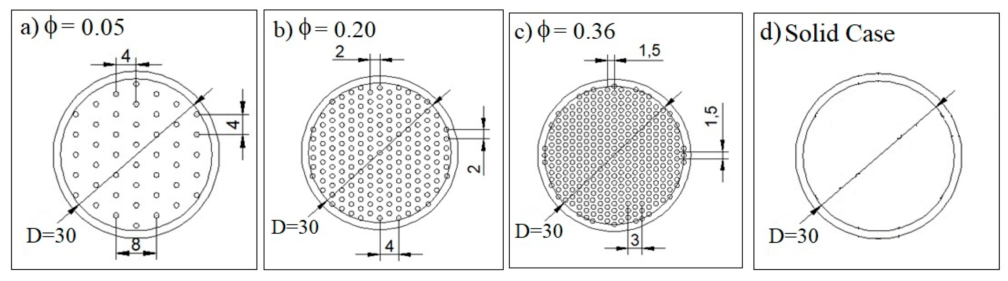
Figure 5.
Schematic sketch of the plants of different densities; (a) ϕ = 0.05, (b) ϕ = 0.20, (c) ϕ = 0.36, (d) Solid Case (units are in cm).
Figure 5.
Schematic sketch of the plants of different densities; (a) ϕ = 0.05, (b) ϕ = 0.20, (c) ϕ = 0.36, (d) Solid Case (units are in cm).

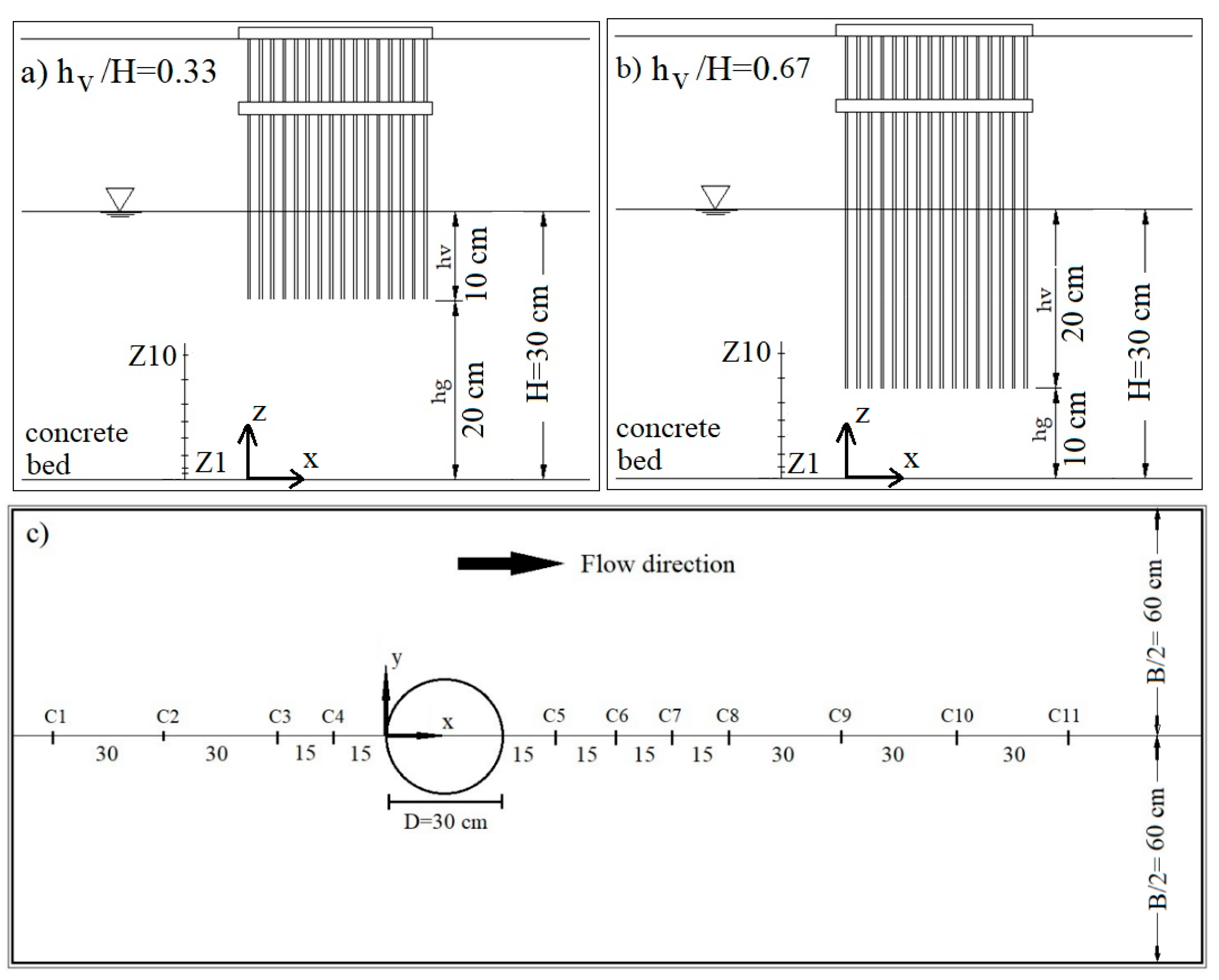
Figure 6.
Velocity measurement points (a) along the flow depth for hv/H = 0.33, (b) along the flow depth for hv/H = 0.67, and (c) along the flow direction (units are in cm).
Figure 6.
Velocity measurement points (a) along the flow depth for hv/H = 0.33, (b) along the flow depth for hv/H = 0.67, and (c) along the flow direction (units are in cm).

Figure 7.
Longitudinal profiles of U velocity for different densities of patches at mid-depth (z/H = 0.5) for (a) h/H = 0.67 and (b) h/H = 0.33.
Figure 7.
Longitudinal profiles of U velocity for different densities of patches at mid-depth (z/H = 0.5) for (a) h/H = 0.67 and (b) h/H = 0.33.

Figure 8.
Longitudinal profiles of V velocity for different densities of patches and depth ratios at mid-depth (z/H = 0.5): (a) ϕ = 0.05, (b) ϕ = 0.20, (c) ϕ = 0.36, (d) Solid Case.
Figure 8.
Longitudinal profiles of V velocity for different densities of patches and depth ratios at mid-depth (z/H = 0.5): (a) ϕ = 0.05, (b) ϕ = 0.20, (c) ϕ = 0.36, (d) Solid Case.


Figure 9.
Vertical profiles of U velocity for different densities of patches along streamwise direction for h/H = 0.67: (a) ϕ = 0.05, (b) ϕ = 0.20, (c) ϕ = 0.36, (d) Solid Case.
Figure 9.
Vertical profiles of U velocity for different densities of patches along streamwise direction for h/H = 0.67: (a) ϕ = 0.05, (b) ϕ = 0.20, (c) ϕ = 0.36, (d) Solid Case.

Figure 10.
Vertical profiles of U velocity for different densities of patches along streamwise direction for h /H = 0.33: (a) ϕ = 0.05, (b) ϕ = 0.20, (c) ϕ = 0.36, (d) Solid Case.
Figure 10.
Vertical profiles of U velocity for different densities of patches along streamwise direction for h /H = 0.33: (a) ϕ = 0.05, (b) ϕ = 0.20, (c) ϕ = 0.36, (d) Solid Case.

Figure 11.
Longitudinal profiles of urms/Udm and vrms/Udm for different densities of patches along the streamwise direction for hv/H = 0.67: (a) ϕ = 0.05, (b) ϕ = 0.20, (c) ϕ = 0.36, (d) Solid Case.
Figure 11.
Longitudinal profiles of urms/Udm and vrms/Udm for different densities of patches along the streamwise direction for hv/H = 0.67: (a) ϕ = 0.05, (b) ϕ = 0.20, (c) ϕ = 0.36, (d) Solid Case.

Figure 12.
Spectral densities of the transverse velocity Sv located at (a) C5 and (b) C11 for Case SVF5 and Solid Case.
Figure 12.
Spectral densities of the transverse velocity Sv located at (a) C5 and (b) C11 for Case SVF5 and Solid Case.


Table 1.
Experimental conditions.
| Cases | a (cm−1) | ϕ | hv/H | Udm (cm/s) | Re | Fr |
|---|---|---|---|---|---|---|
| SVF5 | 0.06 | 0.05 | 0.33 | 11.6 | 35,000 | 0.07 |
| 0.67 | ||||||
| SVF20 | 0.25 | 0.20 | 0.33 | |||
| 0.67 | ||||||
| SVF36 | 0.46 | 0.36 | 0.33 | |||
| 0.67 | ||||||
| Solid Case (SC) | Solid | 1.00 | 0.33 | |||
| 0.67 |
© 2019 by the authors. Licensee MDPI, Basel, Switzerland. This article is an open access article distributed under the terms and conditions of the Creative Commons Attribution (CC BY) license (http://creativecommons.org/licenses/by/4.0/).
Share and Cite
MDPI and ACS Style
Yüksel Ozan, A.; Yılmazer, D. Near-Wake Flow Structure of a Suspended Cylindrical Canopy Patch. Water 2020, 12, 84. https://doi.org/10.3390/w12010084
AMA Style
Yüksel Ozan A, Yılmazer D. Near-Wake Flow Structure of a Suspended Cylindrical Canopy Patch. Water. 2020; 12(1):84. https://doi.org/10.3390/w12010084
Chicago/Turabian StyleYüksel Ozan, Ayşe, and Didem Yılmazer. 2020. "Near-Wake Flow Structure of a Suspended Cylindrical Canopy Patch" Water 12, no. 1: 84. https://doi.org/10.3390/w12010084
Note that from the first issue of 2016, this journal uses article numbers instead of page numbers. See further details here.