Discussion on the Characteristics of Seismic Signals Due to Riverbank Landslides from Laboratory Tests


Department of Soil and Water Conservation, National Chung Hsing University, Taichung 402, Taiwan
*
Author to whom correspondence should be addressed.
Water 2020, 12(1), 83; https://doi.org/10.3390/w12010083
Submission received: 30 November 2019
/
Revised: 20 December 2019
/
Accepted: 21 December 2019
/
Published: 25 December 2019
(This article belongs to the Special Issue The Role of Water in Shallow and Deep Landslides)
Abstract
:Floods and erosion often cause landslides of riverbanks and induce problems such as river blockage, shift of river center, or flooding from rising riverbeds. Instrumentation and monitoring are often used to explore landslide and erosion behavior of riverbanks. Therefore, this study identified landslide types and characteristics of their seismic signals due to toe erosion of riverbanks through riverbank models with various instrumentation sensors in a laboratory flume. To induce landslides in the riverbank model, a test was set up for water to flow through the toe of the riverbank model. Seismic signals of each landslide event were measured during the tests with accelerometers. Nonpolarized electrodes were installed for observing the self-potential changes during the test. Water content and pore water pressure gauges were installed in the riverbank model. In addition, water levels were recorded. The Hilbert–Huang transform method was used to analyze the characteristics of seismic signals caused by water flow and riverbank landslides. Time points, landslide frequency distributions, and the characteristics of several landslide events in the riverbank models were estimated using the seismic signals. This study identified three types of landslides: single, intermittent, and successive. Moreover, changes in self-potential signals, pore water pressure, and water content during the tests were examined and were found to correspond to the landslide process of the riverbank model.
1. Introduction
The toe of riverbanks is often eroded, causing severe landslide events due to strong current and floods. In turn, these influence flow conditions of a river and the nearby facilities. Thus, many mitigation units must monitor and investigate the mechanism of riverbank landslides in order to develop appropriate preventive measures. Many researchers have previously developed various techniques to monitor the conditions and variations of riverbanks. For example, Rosser et al. [1] applied terrestrial laser scanning (TLS) to monitor the process of coastal cliff erosion, Kociuba et al. [2] quantified spatial and temporal transformations of valley floor by TLS, and Longoni et al. [3] applied TLS to monitor riverbank erosion in mountain catchments. TLS provides a high-precision quantification measure for observing retreat and erosion of riverbank and cliff, and it is also very cost-effective.
Studies have also selected pore water pressure and water content for monitoring and discussing landslide mechanisms, and many of them have shown favorable results. Orense et al. [4] conducted a rainfall seepage failure test in a laboratory, and their results showed that occurrences of slope failure could be predicted by monitoring soil water content and pore water pressure changes. Lourenço et al. [5] revealed that pore water pressure decreased continuously during the failure of slope models. Thus, they inferred that changes in pore water pressure were directly related to successive seepage erosion and slump failure. Terajima et al. [6] constructed a slope model in a laboratory for a rainfall infiltration test to understand the mechanism behind shallow landslides induced by rainwater. Arosio et al. [7] applied the electrical resistivity tomography (ERT) technique to perform time-lapse geoelectrical measurements using the Wenner configuration in a small-scale flume for a levee model. Their purpose was to monitor soil saturation variations in levees due to changes in water level in the channel as well as rainfall. Tresoldi et al. [8] monitored long-term water content distribution within a levee using ERT. Rinaldi et al. [9] monitored pore water pressure changes and studied riverbank stability during flow events using a series of tensiometer–piezometers in a riverbank.
In contrast to the ERT method, which uses active direct current for charging the ground during testing, the self-potential method is a passive measurement. Its setup is also simpler than the ERT method. Nonpolarized electrodes containing Pb/PbCl2 or CuSO4 are used to measure the self-potential signals without charging the ground. Revil et al. [10] performed a water infiltration experiment near a ditch and found a linear relationship between the self-potential and depth of the water table. Hottori et al. [11] carried out a laboratory experiment to investigate the rainfall-induced landslide process and concluded that there was a good relationship between self-potential and groundwater condition.
Shinbrot et al. [12] conducted an experiment for slip events of cohesive powder specimens and measured the self-potential changes during the tests. The results indicated that self-potential of the powder specimen changed when it slipped. They concluded that slip events in cohesive powders produce electrical signals, and these signals can appear significantly before the slip events. Hong [13] performed an indoor infiltration experiment and demonstrated that the relationship between the self-potential and water content could be indirectly obtained from the change in self-potential values. Lin [14] conducted a sandbox test and learned that slope failure due to piping caused a decrease in self-potential. The changing pore water pressure mainly caused the change in self-potential. Therefore, self-potential and pore water pressure (or water level) were assumed to be highly correlated.
Seismic signal analysis is very useful in identifying landslide mechanisms. The monitored results can sometimes be used as a precursor of landslides and thus for issuing warnings before landslides. Senfaute et al. [15] studied the precursory seismic signals 15 h prior to rockfall on coastal chalk cliffs. They pointed out that the seismic events showed a progressive decrease in frequency spectrum as the rock cliff approached failure and that application of the seismic monitoring system allowed identification of precursory seismic signals before rockfall. Suwa et al. [16] investigated a landslide event that occurred in Nara, Japan, caused by a rainstorm. The seismic signal received from the observatory revealed that the instrument received surface waves from the landslide site 9 s before the landslide occurred, which was later discovered to be caused by a rupture phenomenon in the slope before the landslide. Therefore, this signal of the preslide rupture phenomenon can be treated as a precursor of the landslide. Dammeier et al. [17] collected seismic signals from 20 known landsides in the middle of the Alps and studied their characteristics. Their findings indicate that the main seismic energy of rockslide is mainly contained in frequencies below 3–4 Hz, while the signal between 3 and 10 Hz may be caused by the impact of huge rocks. The results also indicate that higher frequencies of seismic energy decay earlier. Hibert et al. [18] conducted a study on seismic signals in response to two landslide events on 10 April 2013, at the Bingham Canyon Mine pit. After the seismic signals of both landslide events were received at the nearest monitoring station (MID; 10 km), the seismic wave reached the DUG station (68 km) in approximately 30 s. The study used the Hilbert–Huang transform (HHT) method to analyze the seismic signals received by the DUG monitoring station, and the results revealed that the energy peaked 1 min after receiving the signals and was concentrated at 5 Hz. Provost et al. [19] proposed a classification of seismic signals generated by various types of landslide processes, including slide, fall, topple, and flow. They analyzed duration, frequency content, and spectrogram shape of the seismic sources acquired from 13 unstable slopes and categorized the signals into three main classes—“slope quake”, “rockfall”, and “granular flow”—based on the characteristics of the signals.
Seismic signals recorded near riverbanks are often analyzed to recognize landslide and flood events. Feng [20] interpreted the hydrological processes associated with the Xiaolin landslide and dam-break flooding in 2009 through seismic signals from a broadband station and deduced the duration of the river blockage, time of the dam breach, duration of the flooding surge wave, and average speed of the surge wave. Chao et al. [21] set up seismic array along a river to record the seismic noise due to flow and sediment transport during the typhoon season in 2011. Based on their analyses of spectral characteristics of the seismic signals, they detected 20 landslide or debris flow events near the riverbanks.
Riverbank landslides always produce vibrations and thus seismic signals. The seismic signals correspond to the landslide process in detail, which helps to explain the mechanisms and classify the types of landslides along a riverbank. According to the abovementioned studies, the analysis of seismic signals can provide information on landslide characteristics and time of landslide occurrence as well as vibration frequency contents, spectrogram, and energy. The aim of this study was to identify the types of riverbank landslides based on the characteristics of seismic signals. Spectrograms of seismic signals under different conditions, including background noise and periods of rising water levels, landslides, and water discharge, were compared. The riverbank landslide tests were conducted in a laboratory flume. During testing, accelerometers were installed in the riverbank model for continuous measurement of the seismic signals generated by riverbank landslides. The variations of self-potential signals were recorded by nonpolarized electrodes. Pore water pressure and soil water content were also measured for comparison. Three types of riverbank landslides were identified during the tests: single, intermittent, and successive. In this study, the model rule was not applied; therefore, the field applicability of the proposed results will be used only as a trend result.
2. Methodology
2.1. Test Configuration
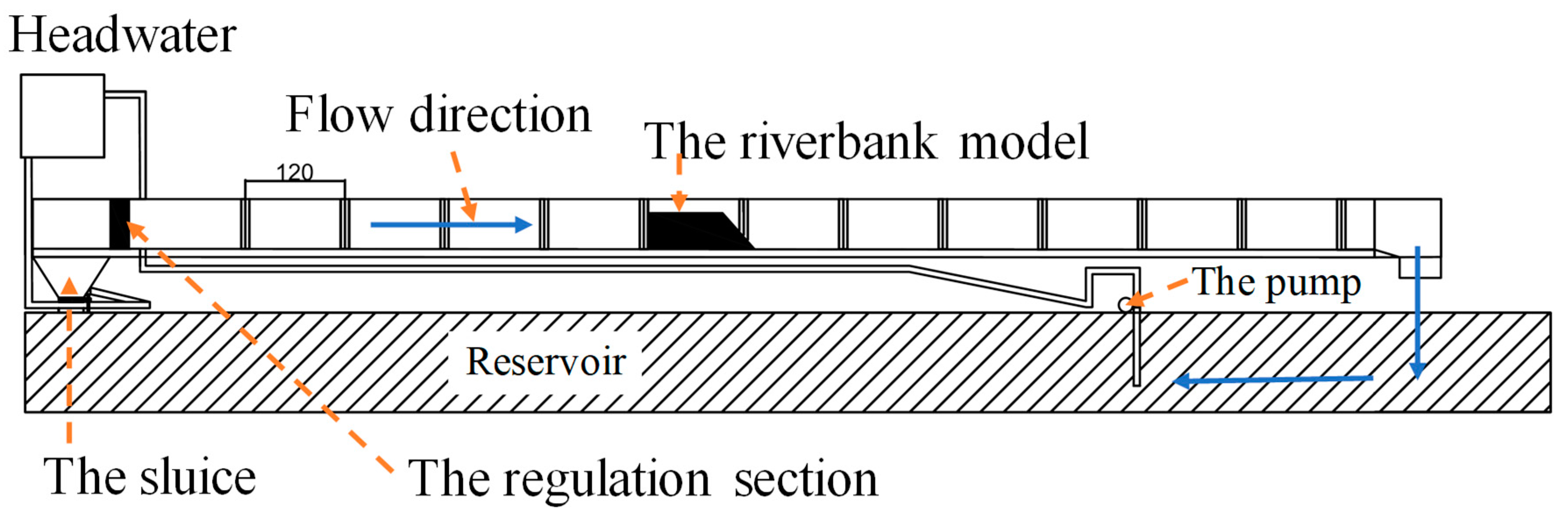
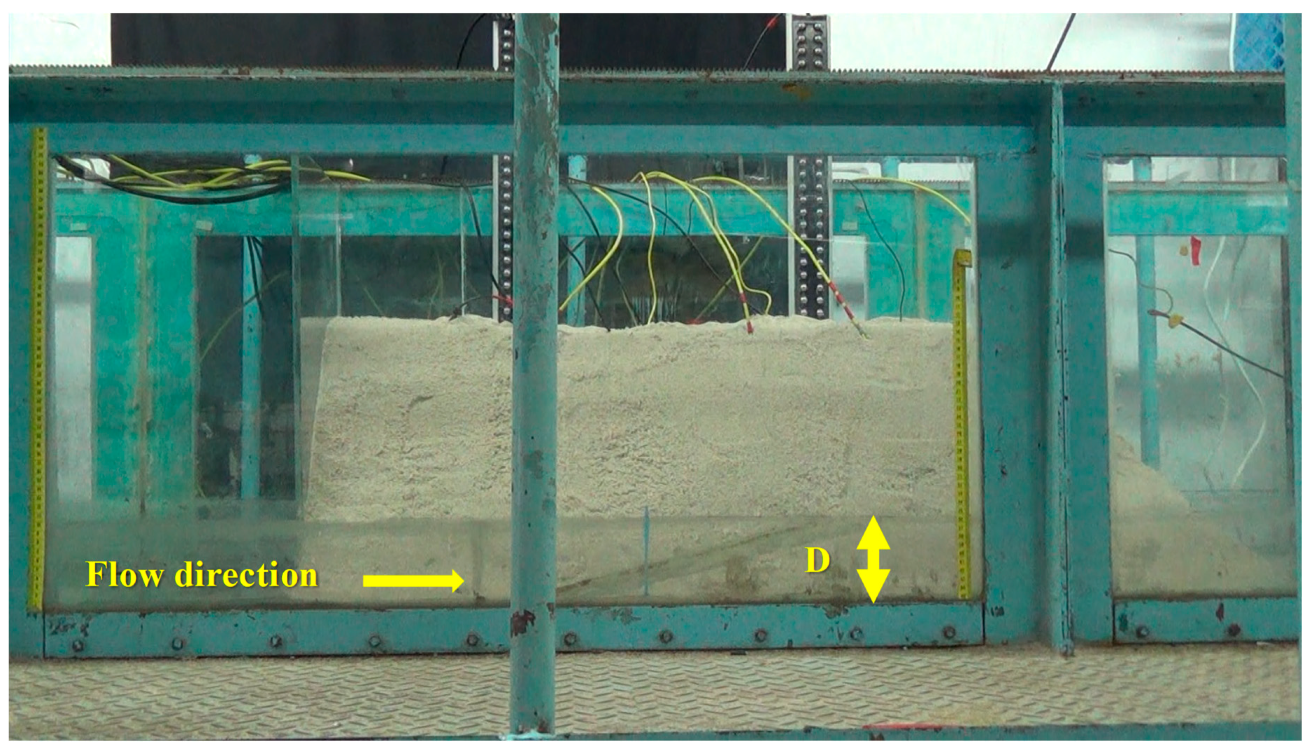
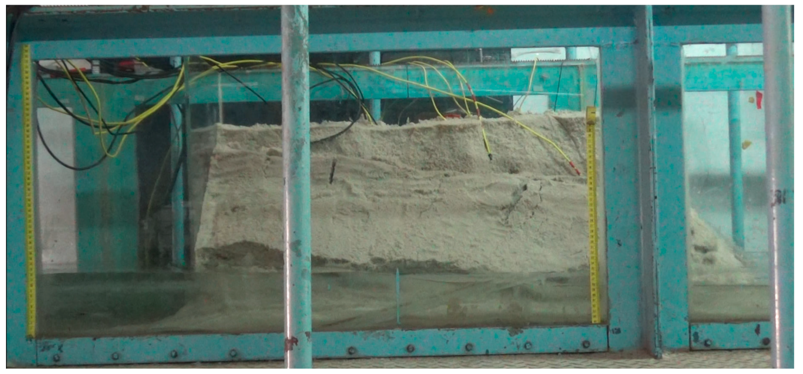
Riverbank models that measured 135 × 50 × 45 (L × W × H) cm were set up in an indoor test flume (Figure 1). The flume measured 15 × 0.6 × 0.6 m and had a slope of 0.1%. A flow pump was used to pump water from the reservoir to the headwater tank, and a sluice was used to control the water level and water flow into the flume. The completed riverbank model is presented in Figure 2, where D is the water flow depth. Table 1 lists the dimensions of the riverbank model.
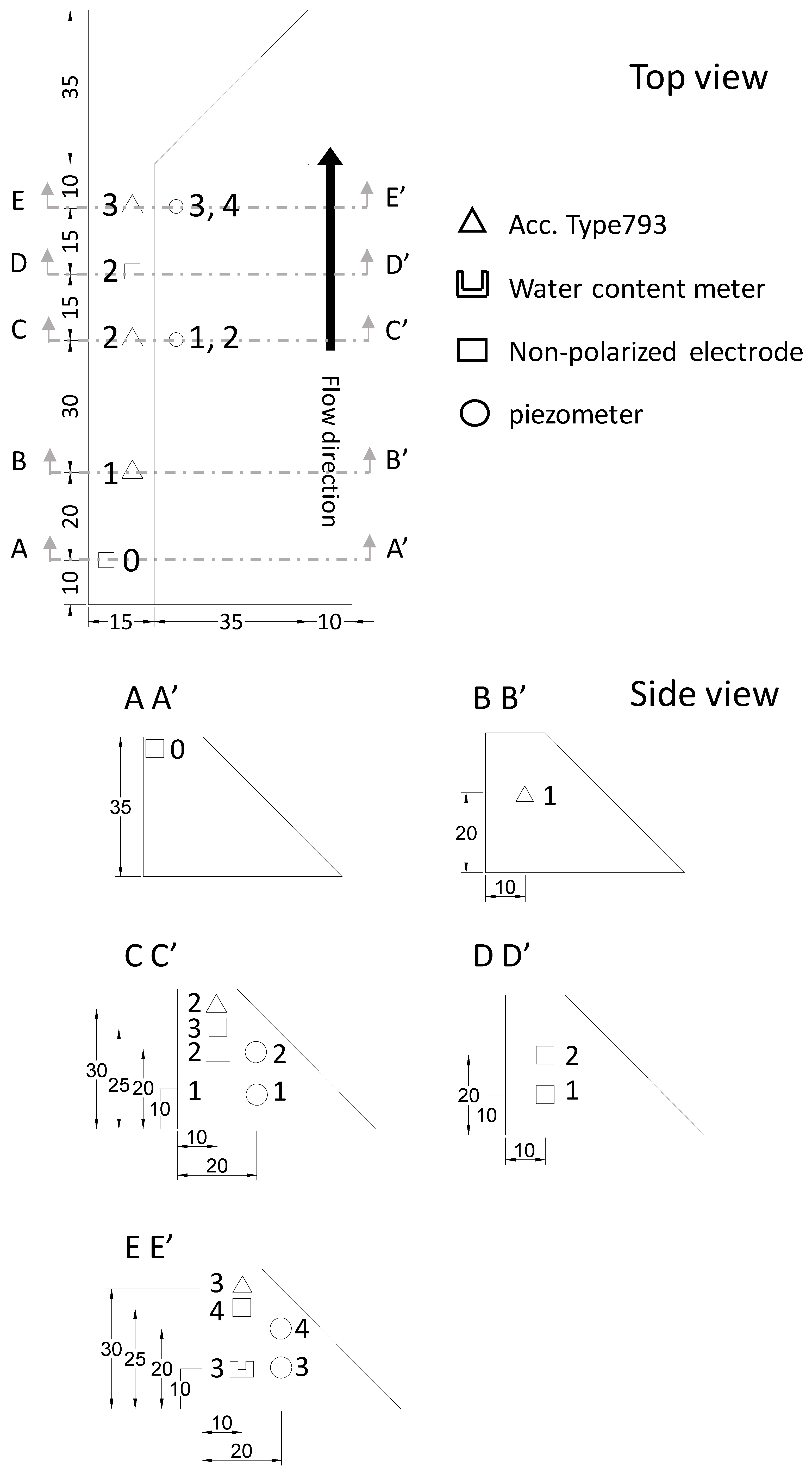
Each sensor was configured as shown in Figure 3 and were numbered for identification. Three increasing operating temperature accelerometers were embedded in the riverbank models to avoid exposure caused by water erosion. The Model 793 accelerometers produced by Wilcoxon Sensing Technologies were used. The frequency response was 1.0–7000 Hz (10%) with sensitivity of 100 mV/g. The sampling rate of the accelerometer was set at 2.5 kHz. Five nonpolarized electrodes were installed (including a negative nonpolarized electrode as the reference electrode) to measure the change in self-potential when the soil was displaced and water contacted a nonpolarized electrode. The reference electrode is numbered “0” in Figure 3. In addition, two piezometers were installed adjacent to the nonpolarized electrodes to measure the riverbank pore pressure changes. Moreover, three soil water content meters were placed adjacent to the piezometers. Cameras were set up at the front and two sides of the model to record the test process and progress of the water flow.
The average grain size of the sands used was 2 mm. Water was evenly added to the sands to maintain stability of the riverbank model. The initial volumetric water contents were measured by water content gauges and were about 7%–19% at various locations in the model. The moisture density of the model was about 1.52 t/m3, and the dry density was 1.34 t/m3. The detailed dimensions of the model can be seen in Figure 3.
At the beginning of the test, water was pumped from the reservoir into the headwater tank. Once the headwater tank was full, the flow pump was turned off to avoid noise. From 0 to 180 s, the background values were measured. At 180 s, tapping was performed to leave a time marker, and the sluice was opened to start discharging the water, with the water depth controlled at a maximum of 15 cm. As the water was drained out at 1030 s, the water was pumped in again during 1030–1500 s, and the test was continued with a water depth at a maximum of 12 cm.
2.2. Analysis Method of Seismic Signal
The seismic signals were analyzed using the Hilbert–Huang transform method, which was proposed by Huang et al. [22]. After observing images of several landslide events in test videos and the related seismic signals generated by the event, an empirical mode decomposition analysis was performed on the seismic signals. A signal can be decomposed into multiple intrinsic mode functions (IMFs), and the Hilbert transform method was used to calculate the spectrogram. Moreover, the power ratio of each IMF and its average frequency can be calculated. The power of IMF is calculated by integrating the square of the signal of IMF. The Visual Signal software package (AnCAD, Inc. [23]) was used to help analyze the seismic signals using HHT.
2.3. Self-Potential Data Measurement and Analysis Method
The self-potential signal measured by the nonpolarized electrode was also analyzed using Visual Signal. Because the original self-potential signal was difficult to observe in the analysis, median filter processing was performed. The median filter is a one-dimensional nonlinear filter that calculates the median of a signal within the filtering range using an equation such as Equation (1) (AnCAD, Inc. [23]).
This equation indicates that, at the center of i positions, points are taken before and after as a series of numbers, and the median of the series is identified to replace the value of i positions of the signal.
Subsequently, the median filtered self-potential signal is calculated using the iterative Gaussian filter. Most of the signals are the combination of periodic and nonperiodic signals, and they can be obtained using the aforementioned filter and applied in Equation (2) (AnCAD, Inc. [23]).
This equation indicates that the value of point is represented by the average of the adjacent points, and the further away it is from point j, the smaller is the weight; σ is a parameter that smooths the window width. The new signal composed of is smoother, that is, its high-frequency part disappears after it is smoothed. Subsequently, the iterative Gaussian filter is applied to ; after several iterations, is obtained (m is the number of iterations), and the sum is a periodic trend signal. At this point, the trend of the self-potential signal should become more noticeable.
3. Results and Discussion
3.1. The Original Measured Signal
3.2. Seismic Signal Characteristics of Three Types of Landslides: Single, Intermittent, and Successive
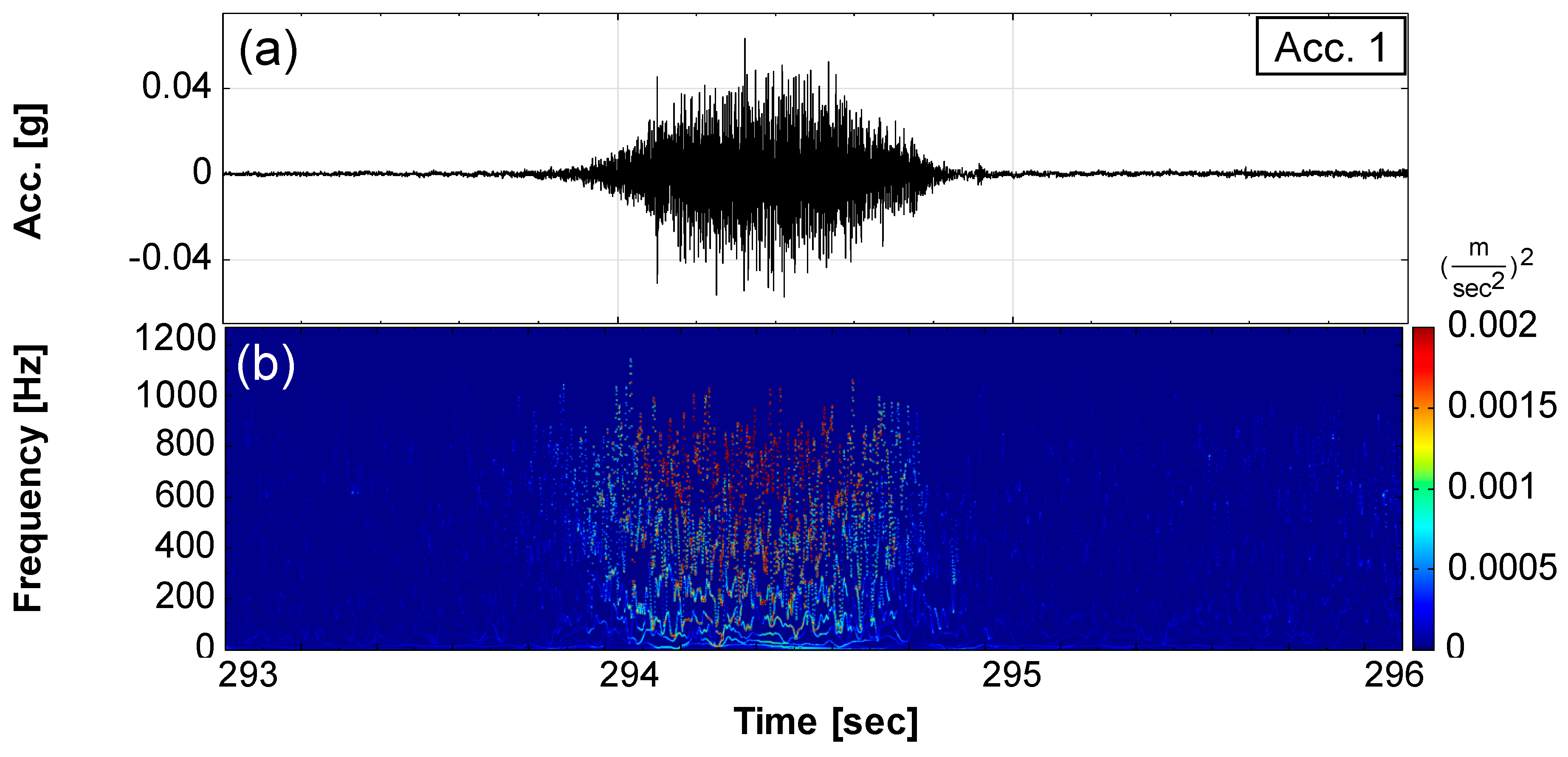
Single landslide: Figure 5 presents an image of landslide Event 1, which was a single landslide that occurred between 293 and 295 s. A single type of landslide caused the soil to slide on the failure surface once, which is the most common type of landslide. Figure 6 and Figure 7 present the seismic signals of accelerometers A1 and A2 and the spectrograms, respectively. The seismic signals revealed that the amplitude reached its peak value approximately 0.2 s after the landslide began; it reduced rapidly afterwards, indicating that Event 1 was short and quick. Moreover, the landslide soil accumulated on the slope toe of the riverbank, causing flow path silting and shifting of the centerline of flow.
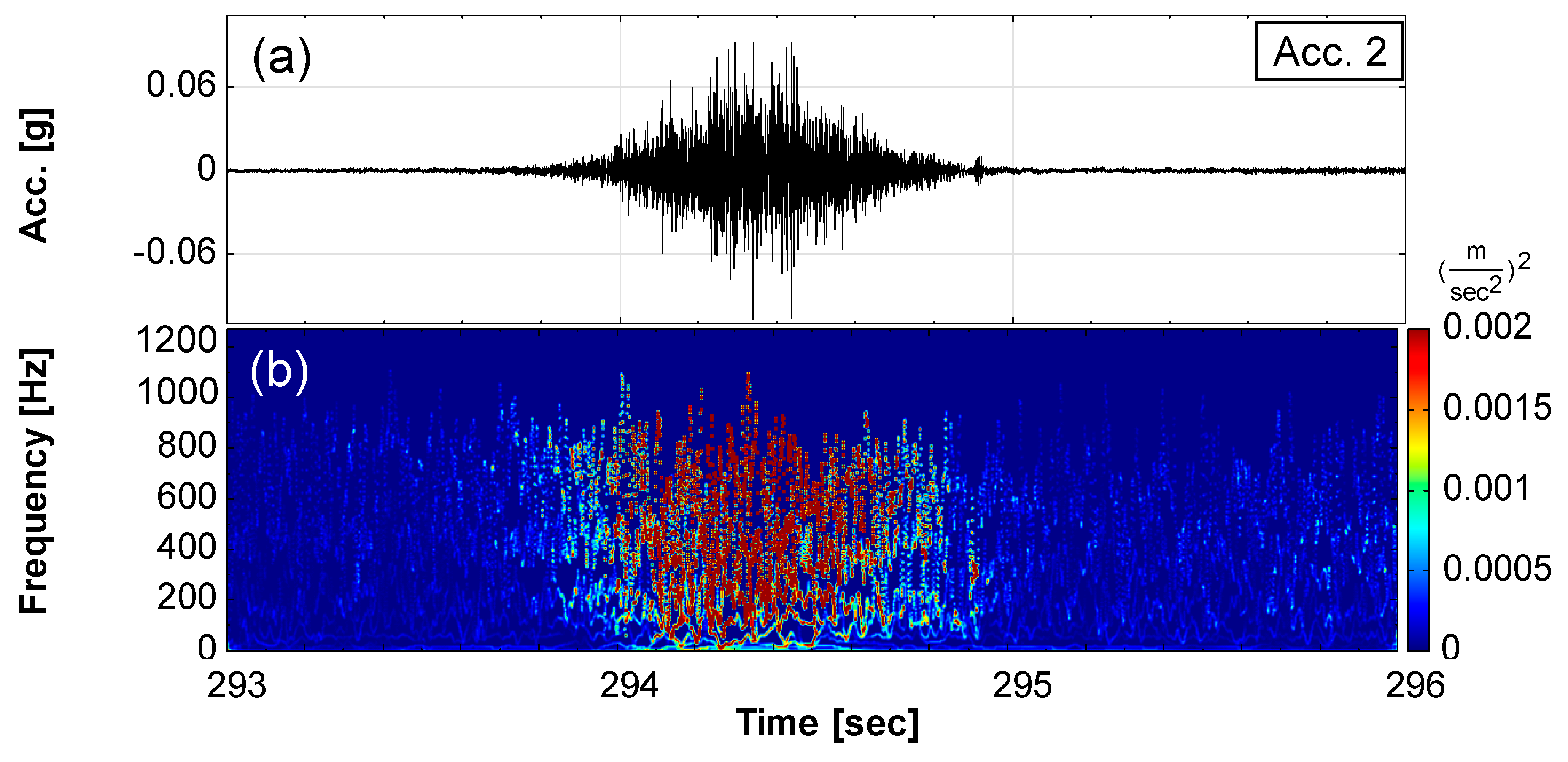
The A2 accelerometer was located farther from the rupture surface of the single slide than A1. The high-frequency energy of A2 was smaller than that of A1 (71.6% < 79.8%, as shown in Table 3). In addition, the high-frequency energy of A1 that concentrated at 840 Hz was also higher than that of A2 at 812 Hz. This proves that high-frequency seismic energy attenuates faster than low-frequency seismic energy in soils.
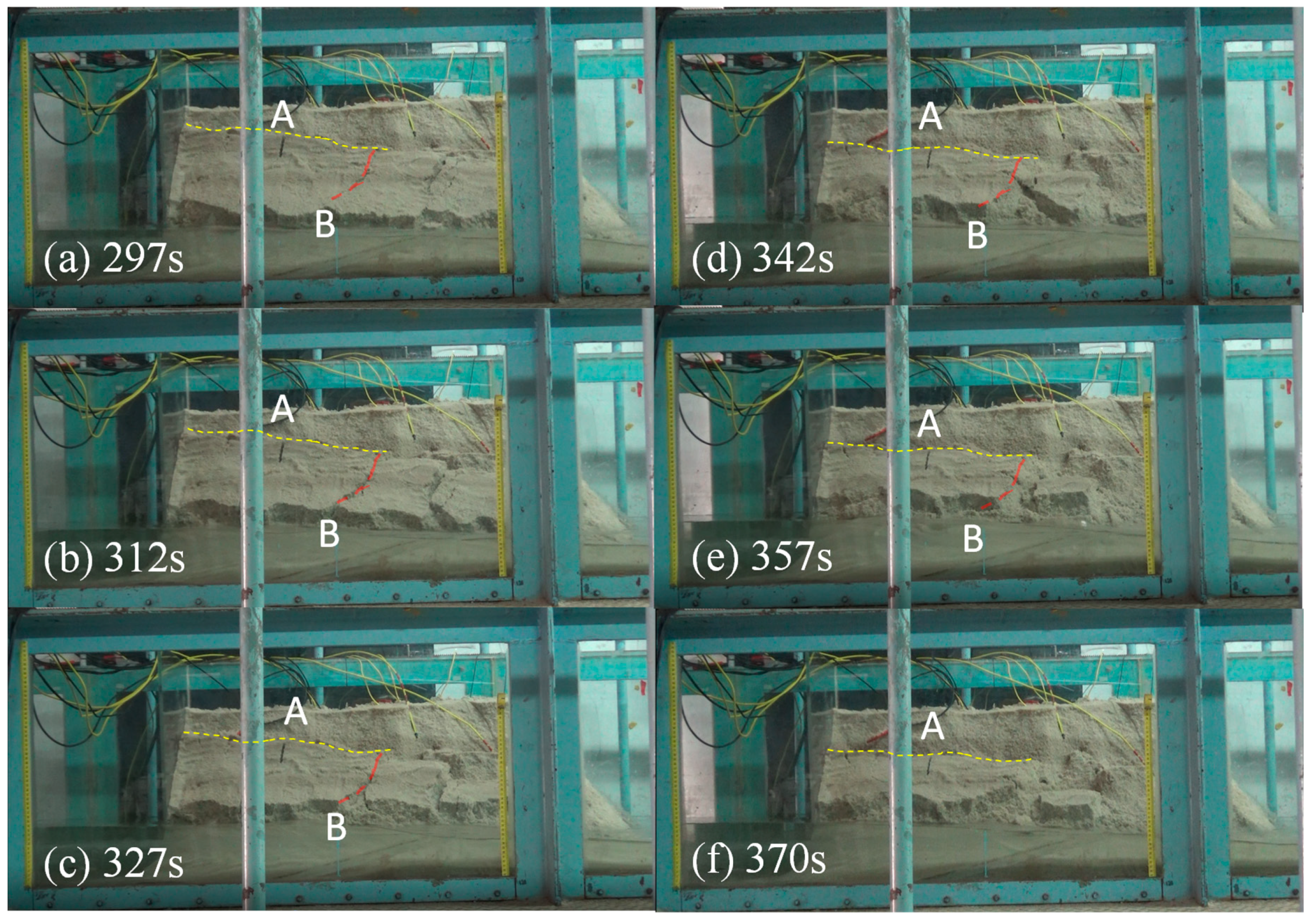
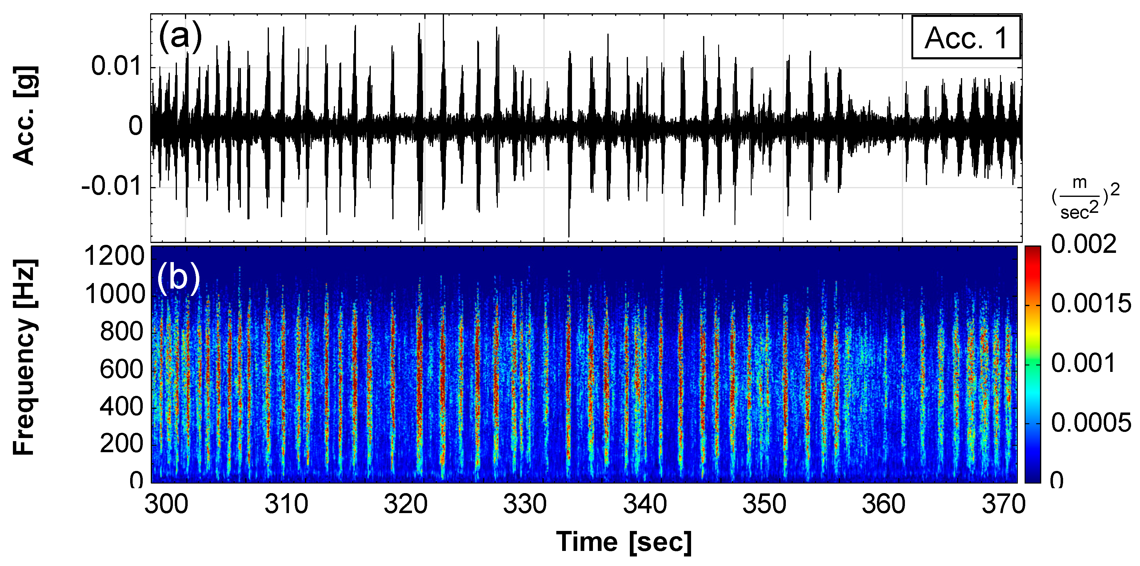
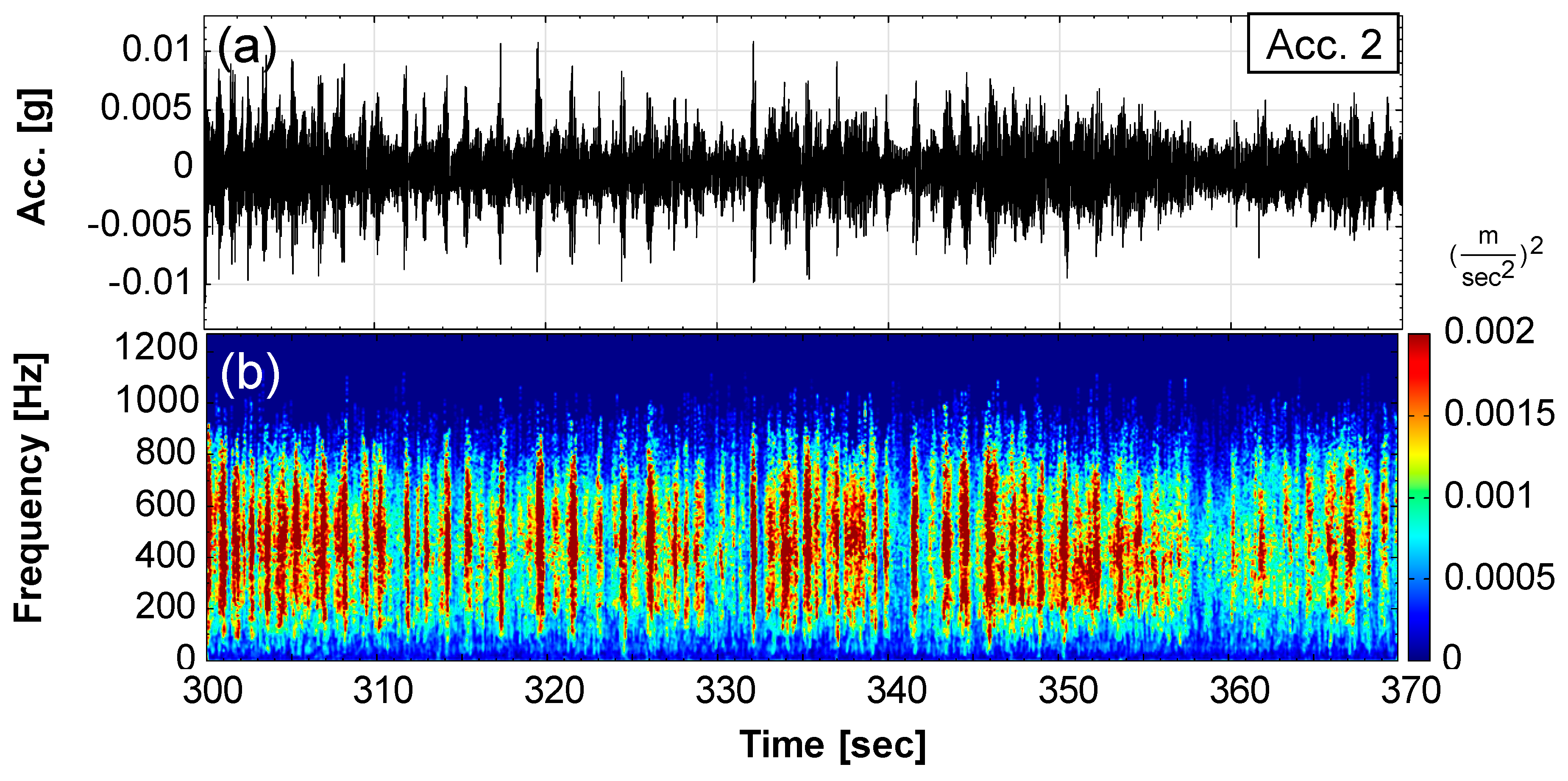
Intermittent landslide: Landslide Event 2 was an intermittent landslide (Figure 8), which refers to the intermittent sliding of soil along the same failure surface. The main scarp A and fissure B of Event 2 are also shown in Figure 8. The process duration of the intermittent landslide Event 2 was approximately 73 s. Figure 9 and Figure 10 present the seismic signals and spectrograms of A1 and A2 from 297 to 370 s, respectively. They reveal that the interval between each landslide was 1–2 s, and the amplitude gradually became smaller at the end of the intermittent landslide. According to the spectral magnitude profile at different times (Figure 11), the landslide energy gradually decreased in the later stage of the intermittent landslide. This study identified a pattern of intermittent landslides, and although it was the result of a laboratory landslide test, this pattern is assumed to occur during actual landslide processes. The difference is that the durations and intervals of actual landslides may occur in months or years. If accelerometers can be installed on actual slopes for monitoring, remediation can be performed if a similar signal is identified. If intermittent landslides occur on an actual slope after a single landslide (like in this study), the early warning effect would be poorer. By contrast, the early warning effect would be more satisfactory if a large-scale landslide occurred after an intermittent landslide. Intermittent landslide signals can be a precursor of a large-scale landslide and can be used to issue a warning for evacuation.
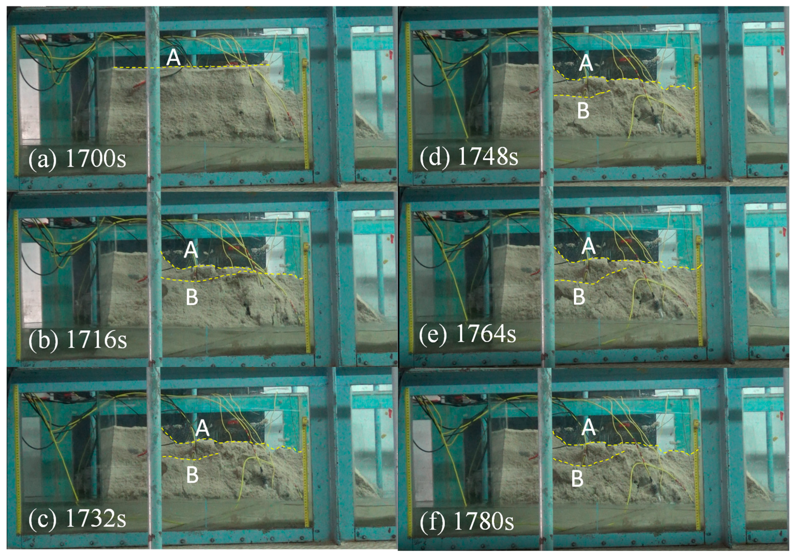
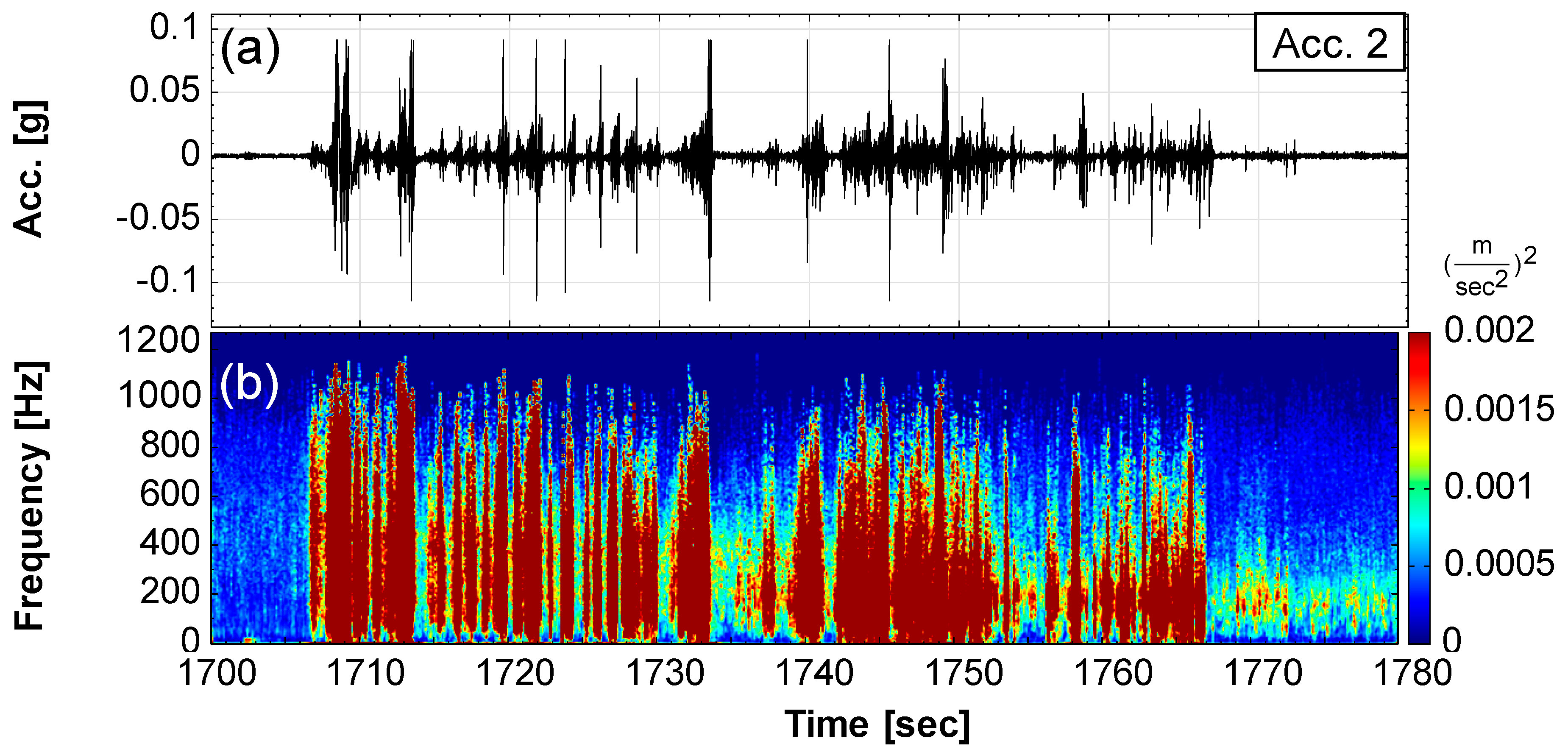
Successive landslide: Landslide Event 3 was a successive landslide (Figure 12), which refers to irregular sliding of soils, where the sliding masses do not share the same value. The irregular sliding masses can slide down on different surfaces. Figure 13 and Figure 14 depict the seismic signals and spectrograms of A1 and A2 from 1700 to 1780 s, respectively. Event 3 lasted for approximately 80 s, and it was observed that the soils sliding successively were different from those sliding down on different failure surfaces. Comparing the seismic signals of successive and intermittent landslides (Figure 13 and Figure 14 with Figure 9 and Figure 10), both seismic signals were similar and were generated at intervals. The signal intervals of the successive landslide were random.
3.3. Correspondence between Variation of Self-Potential, Water Content, and Seismic Signals
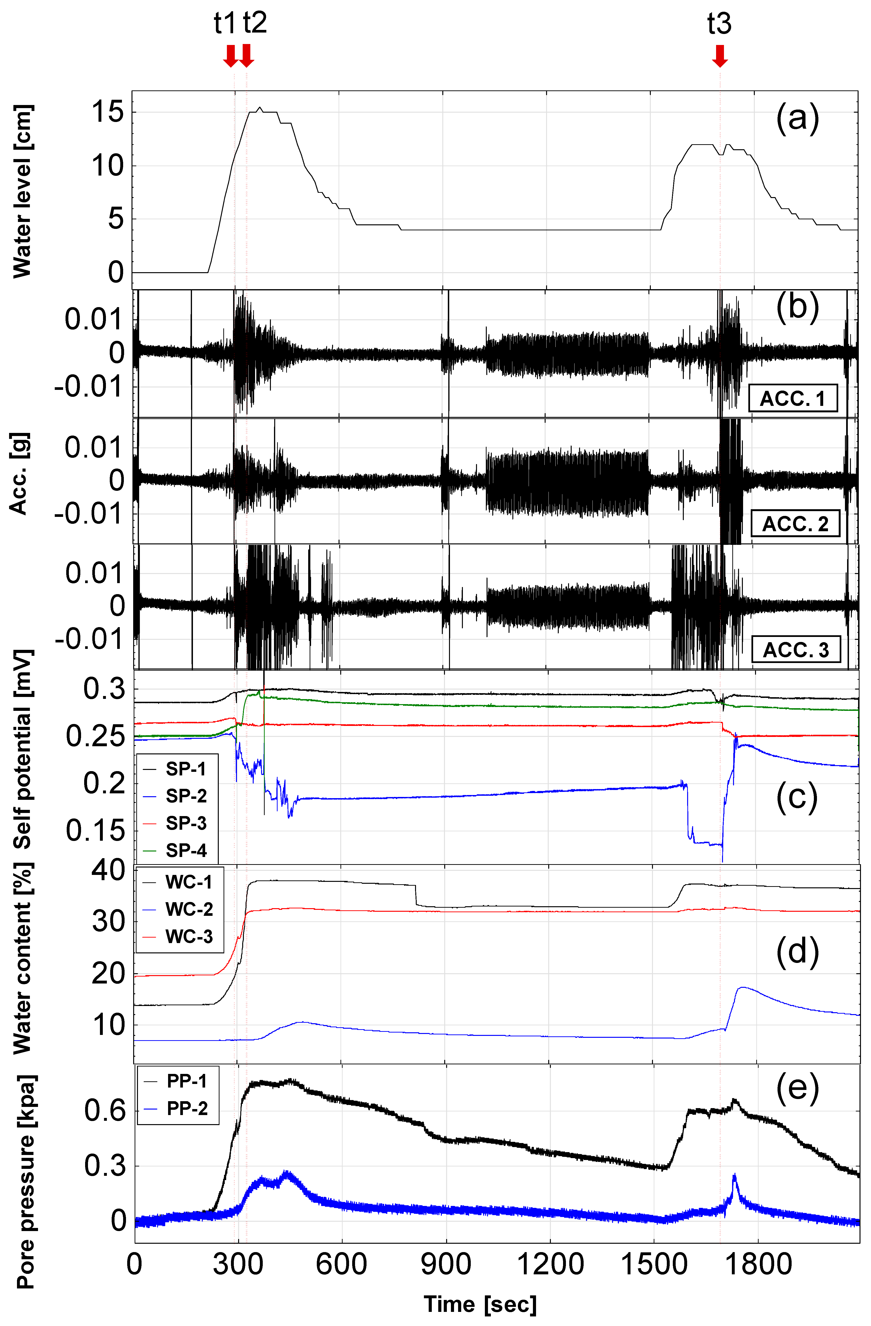
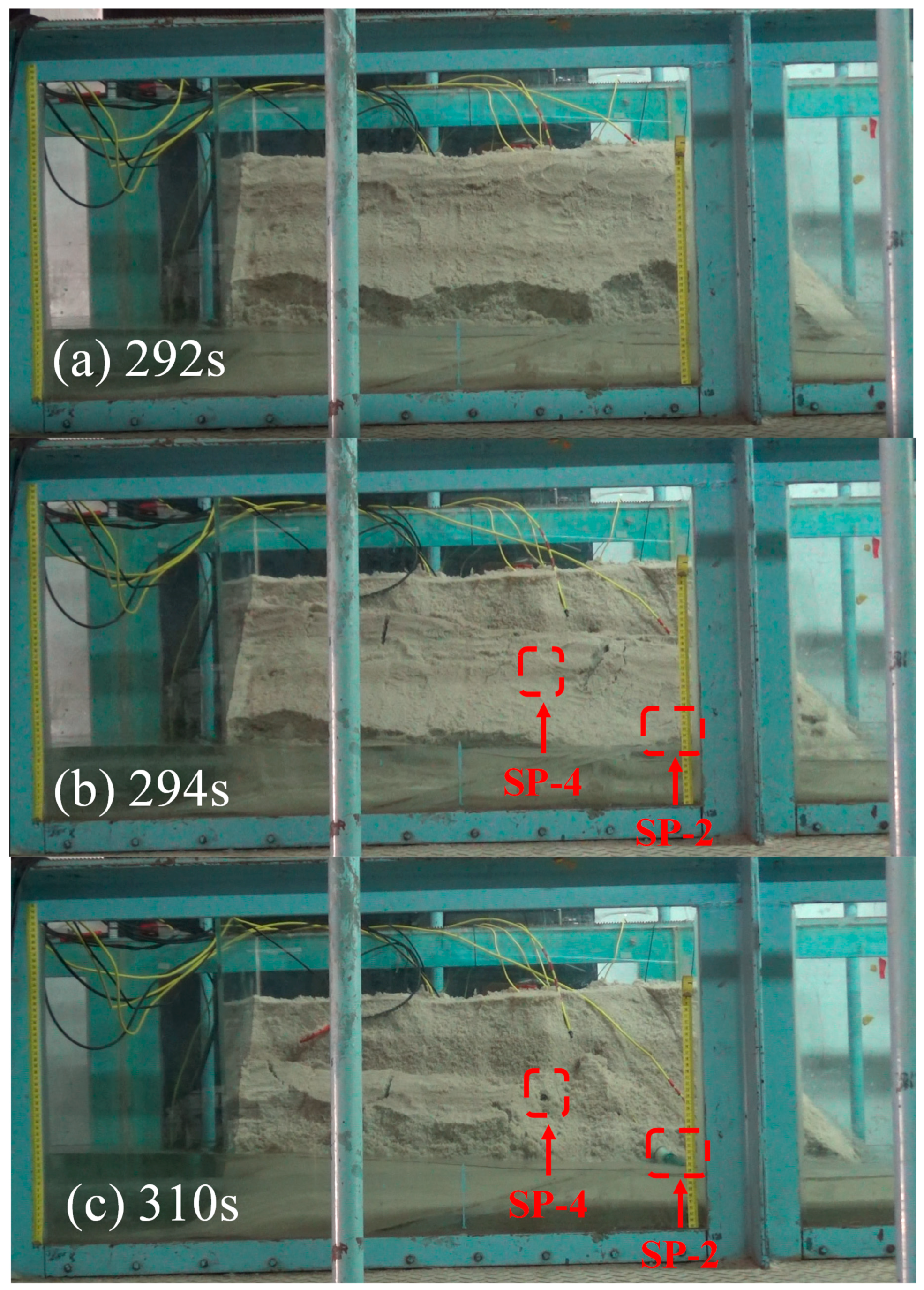
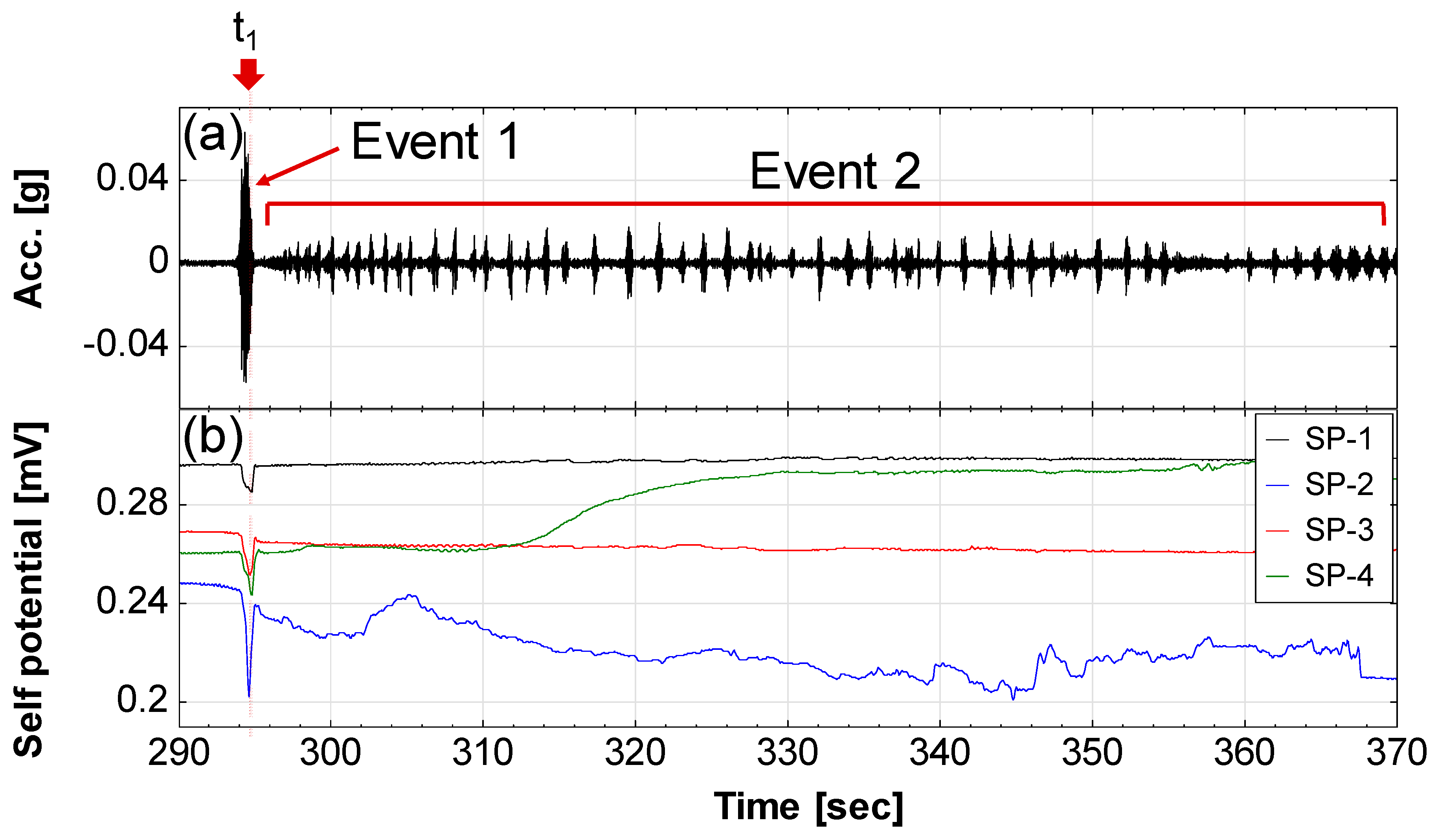
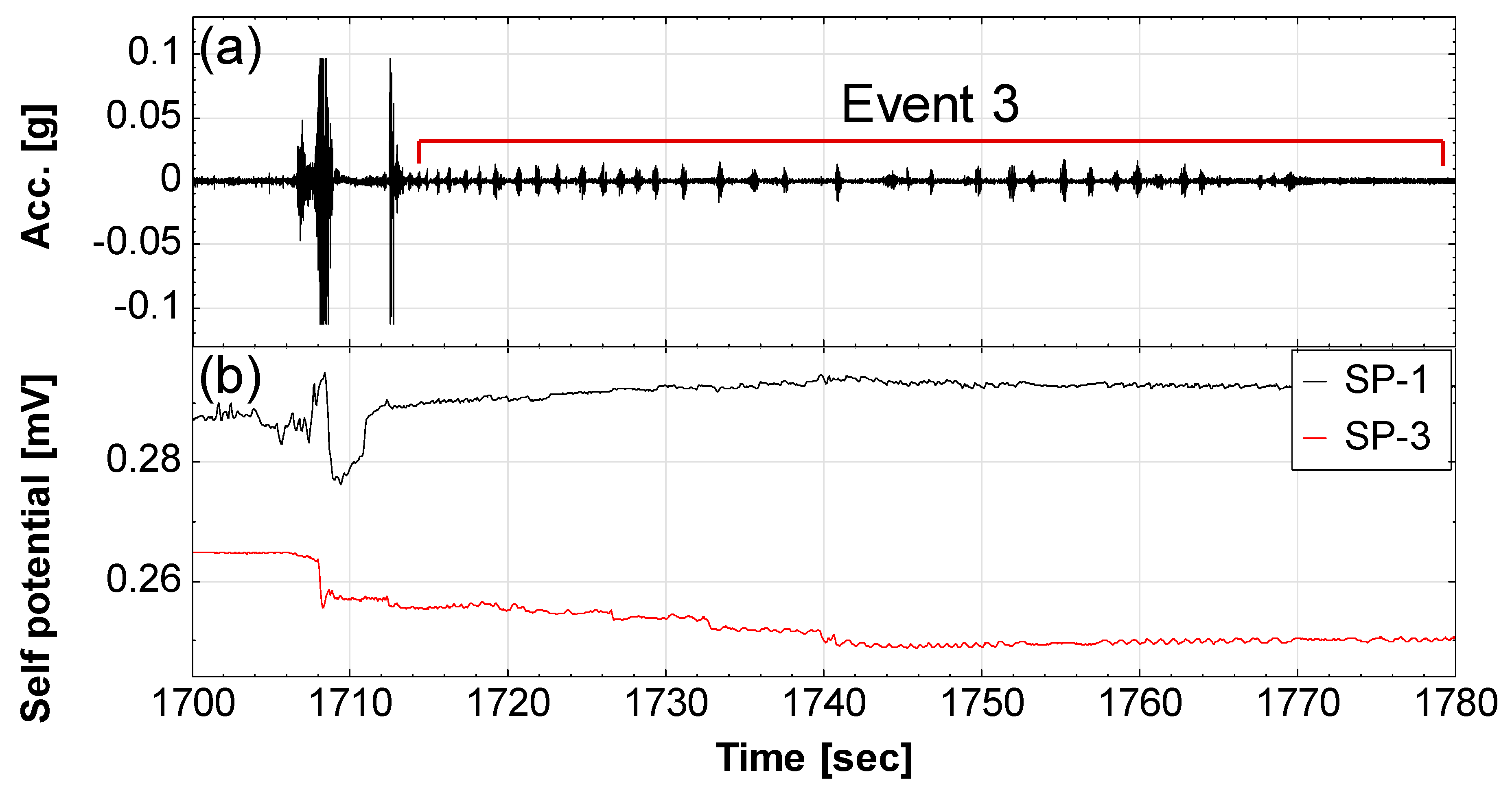
As can be seen in Figure 4c, when the water level in the soil rose slowly to the height of SP-1–SP-4, the self-potential also gradually increased. Comparing self-potential with the soil water content, we found that the self-potential could reflect the time the seepage water level reached the electrode. However, the signal response times might differ because of the different positions of the sensors. A single landslide that occurred during T1 (294 s) produced a seismic signal with a large amplitude, and the self-potential exhibited a signal that rose after an instant drop (i.e., the occurrence of the 294 s landslide could be indicated by the self-potential). At 305 s, the eroded soil caused air exposure at the bottom of SP-4, resulting in a gradual increase in self-potential (Figure 15c). According to the seismic signal of A1 (Figure 16a), Event 2 was an intermittent landslide, and its signal amplitude gradually decreased with time. In addition, the signal of SP-2, which was affected by the intermittent landslide (Figure 16b), exhibited continuous fluctuations, which could reflect the duration of the intermittent landslide. SP-1 and SP-3 did not exhibit such fluctuations because their electrodes were embedded deeper inside the riverbank model and were thus less affected by soil displacement. Event 3 was a successive landslide (Figure 17a), and the single landslide that occurred at 1708 s produced a seismic signal with a large amplitude. The self-potential of SP-1 exhibited a decreasing signal that rose again. SP-1 was still embedded in the soil after the landslide (Figure 17b). Regarding SP-3, its self-potential decreased without rising again because the electrode was exposed in the air during the slide at 1708 s. According to the above discussion, we can conclude that seismic signals are able to reflect the scale and timing of landslide events as well as changes in self-potential corresponding to the timing and location of landslide events (i.e., the location of the nonpolarized electrode).
3.4. Comparison of Seismic Signal Spectrograms
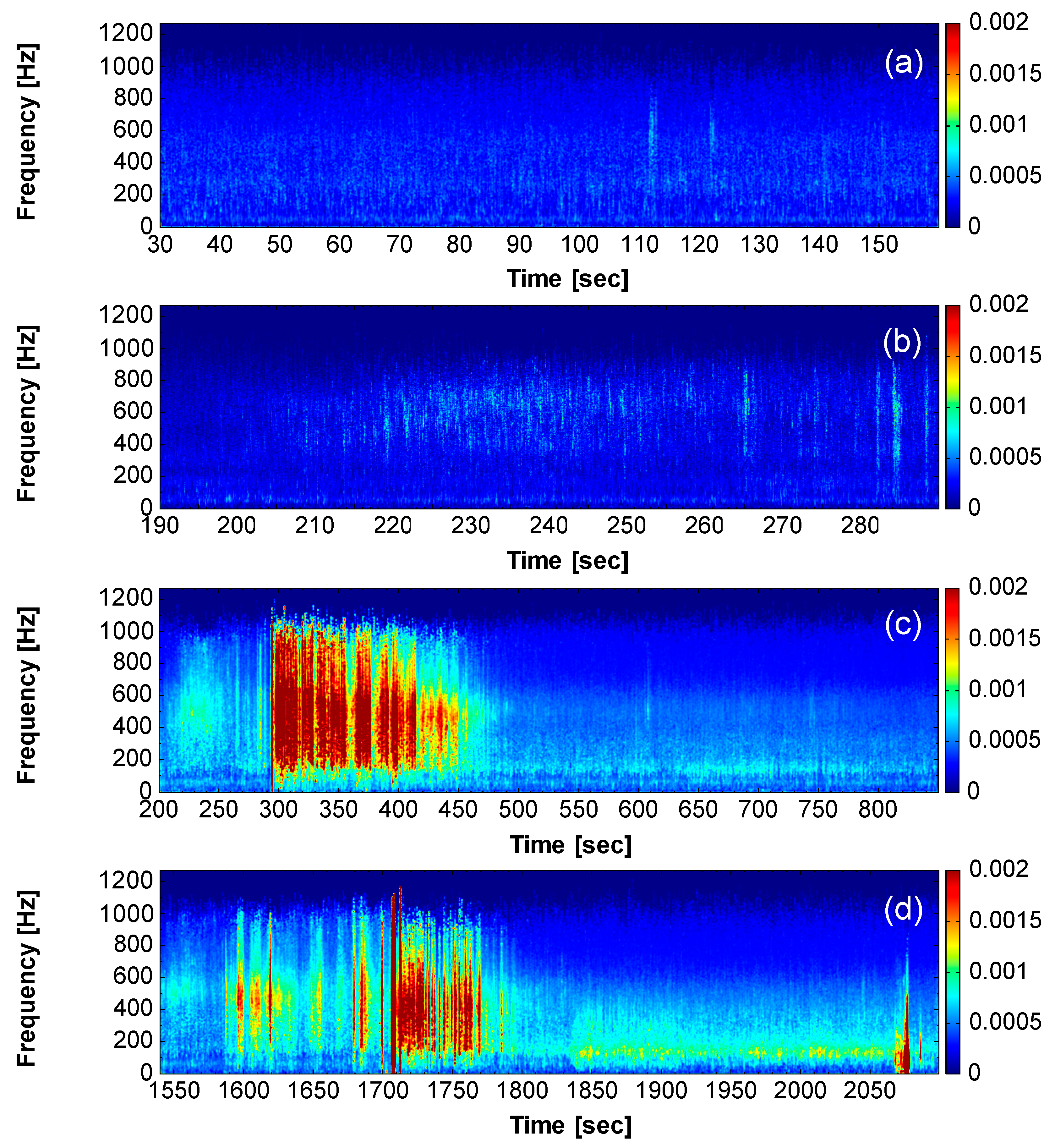
The relationship between the spectrogram of the A1 seismic signal (Figure 18) and experimental conditions was investigated using four durations. First, 30–160 s was selected as Duration No. 1, which was the environmental background value without water flow and landslides in the test. The background value frequencies calculated were mostly concentrated at 831 Hz with an IMF energy ratio of 27.6%. The spectrogram of Duration No. 1 is shown in Figure 18a; only some noise could be detected, and the energy was less noticeable. Duration No. 2 was when the water level rose from 190 to 290 s without landslides; the spectrogram (Figure 18b) indicated that the water flow energy was between 400 and 700 Hz, and its vibration frequency was concentrated at 793 Hz with an IMF energy ratio of 53.6%. Duration No. 3 was the period where single and intermittent landslides and water flow vibration occurred between 200 and 850 s during the first water discharge. Its spectrogram (Figure 18c) exhibited the water flow energy before landslides, during single and intermittent landslides, and after the water flow energy had subsided. The frequency of Duration No. 3 concentrated at 796 Hz with an IMF energy ratio of 69.9%. Duration No. 4 was where single and successive landslides and water flow vibration occurred between 1550 and 2050 s during the second discharge. The frequency of Duration No. 3 concentrated at 761 Hz with an IMF energy ratio of 33.5%. Similarly, its spectrogram (Figure 18d) exhibited the water flow energy before landslides, during the single and successive landslides, and after the water flow energy had subsided.
3.5. Effect of Water Depth
To examine the effect of water depth, we conducted an additional test at a maximum water level of 10 cm. The results revealed that this lower water level had a lower erosion capacity, which caused less landslides than a higher water level of 15 cm and produced a smaller landslide range. However, under the low water level condition, single, intermittent, and successive landslides were also detected along the riverbank model.
3.6. Results of Water Content and Pore Water Pressure
The initial water contents of the riverbank models were measured before the test, with WC-1, WC-2, and WC-3 being approximately 14%, 7%, and 19.5%, respectively (Figure 4d). At 240 s, the water content of WC-1 and WC-3 rose to 38% and 33%, respectively. At 340 s, the embedded location of WC-2 was displaced because of the sliding soil during the T1 (294 s) landslide event, which caused the WC-2 water content to rise. The water content of WC-1 gradually decreased from 815 to 1545 s because the water level decreased, which was caused by complete initial water discharge. At 1545 s, when the water flow was released for the second time, WC-1 again contacted the water surface, which caused the water content to rise again. At T3 (1708 s), after a single landslide occurred at 1710 s, WC-2 was displaced down to the water level with the sliding soil, causing the water content to rise rapidly. Therefore, reasonable linear corrections were performed for the pore pressure data, as shown in Figure 4e. The pore water pressure of PP-1 rose when the water level was higher than the embedded location at 226 s (PP-1 was embedded 10 cm from the flume bottom). The location of PP-2 was gradually displaced downwards due to the intermittent landslide (297 and 370 s), which increased the pore water pressure of PP-2. The water flow was opened for the second time at 1530 s. When the water level reached 5 cm at 1545 s and higher than the elevation of PP-1, the water pressure of PP-1 slowly increased. At 1727 s, the piezometers (PP-1 and PP-2) were flushed out with the sliding soils and ended the measurement of pore pressure.
4. Conclusions
In this study, riverbank toe erosion tests were conducted in a laboratory, and the seismic signals, self-potential responses, pore water pressures, and water levels were measured. The measurement results were analyzed, and the conclusions drawn are discussed below:
- [1]
- Three types of riverbank slope landslides during erosion were identified: (a) single landslide: soil sliding down on one failure surface once; (b) intermittent landslide: soil gradually sliding down along the same sliding surface intermittently; and (c) successive landslide: different soils continuously sliding down from different sliding surfaces. The characteristics and processes of these three types of landslides corresponded to their seismic signals and spectrograms. The seismic signals can be used to clearly indicate the timing of landslide occurance.
- [2]
- The occurrence intervals of the intermittent landslides in this study were approximately 1–2 s in the test. Seismic signals can be monitored by means of accelerometers and velocimeters on an actual slope for landslide events. The monitored signals are helpful for identifying landslide events and have the potential to provide early landslide warnings.
- [3]
- High-frequency seismic energy attenuates faster than low-frequency seismic energy.
- [4]
- Self-potential can be used to indicate the timing of landslide events and the time when the water level contacts the electrode. Based on changes in self-potential, it was noted that self-potential rose gradually as the water level rose to make contact with the nonpolarized electrode. The self-potential dropped instantly and jumped back again when a landslide occurred near the electrode. The self-potential decreased continuously when the electrode slid down with the soil.
- [5]
- In the case of higher water level (15 cm) flow, the riverbank slope exhibited a greater landslide range with more soils. However, in the case of a lower water level (10 cm), the landslide range was smaller because of a lower erosion capacity.
Supplementary Materials
The following are available online at https://www.mdpi.com/2073-4441/12/1/83/s1, Video S1: Event 1 single landslide; Video S2: Event 2 intermittent landslide; Video S3: Event 3 successive landslide.
Author Contributions
Methodology, formal analysis, investigation, supervision, writing—original draft Z.-Y.F.; Data curation, formal analysis, investigation, visualization, C.-M.H.; Data curation, formal analysis, visualization, S.-H.C. All authors have read and agreed to the published version of the manuscript.
Funding
This research was funded by the Ministry of Science and Technology, Taiwan, R.O.C, grant number 107-2625-M-005-007.
Acknowledgments
The authors acknowledge the Ministry of Science and Technology, Taiwan, R.O.C, for providing research funding (grant number: 107-2625-M-005-007). The authors acknowledge Su-chin Chen of the Department of Soil and Water Conservation, National Chung Hsing University, for providing the test flume used for the experiments. The constructive comments from the reviewers are much appreciated. Acknowledgments are also extended to Samkele Tfwala for reviewing the manuscript style.
Conflicts of Interest
The authors declare no conflict of interest.
References
- Rosser, N.J.; Petley, D.N.; Lim, M.; Dunning, S.A.; Allison, R.J. Terrestrial laser scanning for monitoring the process of hard rock coastal cliff erosion. Q. J. Eng. Geol. Hydrogeol. 2005, 38, 363–375. [Google Scholar] [CrossRef]
- Kociuba, W.; Kubisz, W.; Zagórski, P. Use of terrestrial laser scanning (TLS) for monitoring and modelling of geomorphic processes and phenomena at a small and medium spatial scale in Polar environment (Scott River—Spitsbergen). Geomorphology 2014, 212, 84–96. [Google Scholar] [CrossRef]
- Longoni, L.; Papini, M.; Brambilla, D.; Barazzetti, L.; Roncoroni, F.; Scaioni, M.; Ivanov, V.I. Monitoring riverbank erosion in mountain catchments using terrestrial laser scanning. Remote Sens. 2016, 8, 241. [Google Scholar] [CrossRef] [Green Version]
- Orense, R.P.; Shimoma, S.; Maeda, K.; Towhata, I. Instrumented model slope failure due to water seepage. J. Nat. Disaster Sci. 2004, 26, 15–26. [Google Scholar] [CrossRef] [Green Version]
- Lourenço, S.D.; Sassa, K.; Fukuoka, H. Failure process and hydrologic response of a two layer physical model: Implications for rainfall-induced landslides. Geomorphology 2006, 73, 115–130. [Google Scholar] [CrossRef]
- Terajima, T.; Miyahira, E.I.; Miyajima, H.; Ochiai, H.; Hattori, K. How hydrological factors initiate instability in a model sandy slope. Hydrol. Process. 2014, 28, 5711–5724. [Google Scholar] [CrossRef] [Green Version]
- Arosio, D.; Hojat, A.; Ivanov, V.I.; Loke, M.H.; Longoni, L.; Papini, M.; Tresoldi, G.; Zanzi, L. A laboratory experience to assess the 3D effects on 2D ERT monitoring of river levees. In Proceedings of the 24th European Meeting of Environmental and Engineering Geophysics, Porto, Portugal, 9–12 September 2018. [Google Scholar]
- Tresoldi, G.; Arosio, D.; Hojat, A.; Longoni, L.; Papini, M.; Zanzi, L. Long-term hydrogeophysical monitoring of the internal conditions of river levees. Eng. Geol. 2019, 259, 105139. [Google Scholar] [CrossRef]
- Rinaldi, M.; Casagli, N.; Dapporto, S.; Gargini, A. Monitoring and modelling of pore water pressure changes and riverbank stability during flow events. Earth Surf. Process. Landf. 2004, 29, 237–254. [Google Scholar] [CrossRef]
- Revil, A.; Hermitte, D.; Voltz, M.; Moussa, R.; Lacas, J.G.; Bourrié, G.; Trolard, F. Self-potential signals associated with variations of the hydraulic head during an infiltration experiment. Geophys. Res. Lett. 2002, 29, 10–11. [Google Scholar] [CrossRef]
- Hattori, K.; Kohno, H.; Tojo, Y.; Terajima, T.; Ochiai, H. Early warning of landslides based on landslide indoor experiments. In Ch. 20.8 of Landslides—Disaster Risk Reduction Monitoring; Sassa, K., Canuti, P., Eds.; Springer: Berlin/Heidelberg, Germany, 2009; pp. 363–366. ISBN 978-3-540-69970-5. [Google Scholar]
- Shinbrot, T.; Kim, N.H.; Thyagu, N.N. Electrostatic precursors to granular slip events. Proc. Natl. Acad. Sci. USA 2012, 109, 10806–10810. [Google Scholar] [CrossRef] [PubMed] [Green Version]
- Hong, J.L. Monitoring of the Infiltration Process of Shallow Soil Layer by Using Self-Potential Method. Master’s Thesis, National Central University, Taoyuan City, Taiwan, 2014; 77p. (In Chinese). [Google Scholar]
- Lin, C.W. Assessment of Saturation Triggered Slope Failure by Using Self-Potential Measurements and FLAC3D Numerical Model. Master’s Thesis, National Central University, Taoyuan City, Taiwan, 2016; 88p. (In Chinese). [Google Scholar]
- Senfaute, G.; Duperret, A.; Lawrence, J.A. Micro-seismic precursory cracks prior to rock-fall on coastal chalk cliffs: A case study at Mesnil-Val, Normandie, NW France. Nat. Hazards Earth Syst. Sci. 2009, 9, 1625–1641. [Google Scholar] [CrossRef]
- Suwa, H.; Mizuno, T.; Ishii, T. Prediction of a landslide and analysis of slide motion with reference to the 2004 Ohto slide in Nara, Japan. Geomorphology 2010, 124, 157–163. [Google Scholar] [CrossRef]
- Dammeier, F.; Moore, J.R.; Haslinger, F.; Loew, S. Characterization of alpine rockslides using statistical analysis of seismic signals. J. Geophys. Res. Earth Surf. 2011, 116, F04024. [Google Scholar] [CrossRef]
- Hibert, C.; Ekström, G.; Stark, C.P. Dynamics of the Bingham Canyon Mine landslides from seismic signal analysis. Geophys. Res. Lett. 2014, 41, 4535–4541. [Google Scholar] [CrossRef]
- Provost, F.; Malet, J.P.; Hibert, C.; Helmstetter, A.; Radiguet, M.; Amitrano, D.; Langet, N.; Larose, E.; Abancó, C.; Hürlimann, M.; et al. Towards a standard typology of endogenous landslide seismic sources. Earth Surf. Dyn. 2018, 6, 1059–1088. [Google Scholar] [CrossRef] [Green Version]
- Feng, Z.Y. The seismic signatures of the surge wave from the 2009 Xiaolin landslide-dam breach in Taiwan. Hydrol. Process. 2012, 26, 1342–1351. [Google Scholar] [CrossRef]
- Chao, W.A.; Wu, Y.M.; Zhao, L.; Tsai, V.C.; Chen, C.H. Seismologically determined bedload flux during the typhoon season. Sci. Rep. 2015, 5, 8261. [Google Scholar] [CrossRef] [PubMed] [Green Version]
- Huang, N.E.; Shen, Z.; Long, S.R.; Wu, M.C.; Shih, H.H.; Zheng, Q.; Yen, N.C.; Tung, C.C.; Liu, H.H. The empirical mode decomposition and the Hilbert spectrum for nonlinear and nonstationary time series analysis. Proc. R. Soc. Lond. Ser. A Math. Phys. Eng. Sci. 1998, 454, 903–995. [Google Scholar] [CrossRef]
- AnCAD, Inc. Visual Signal Reference Guide, Version1.5. Available online: http://www.ancad.com.tw/ (accessed on 24 August 2019). (In Chinese).
Figure 1.
Layout of the test flume.

Figure 2.
The side view of the riverbank model.

Figure 3.
Sensor configuration in the riverbank model.

Figure 4.
Original signal of the measurements: (a) water level, (b) accelerometer A1 seismic signal, (c) self-potential, (d) water content, (e) pore pressure.
Figure 4.
Original signal of the measurements: (a) water level, (b) accelerometer A1 seismic signal, (c) self-potential, (d) water content, (e) pore pressure.

Figure 5.
Before and after images of the single slide (Event 1).

Figure 6.
Accelerometer A1, Event1 (293–295 s): (a) original seismic signal, (b) time-frequency spectrogram.
Figure 6.
Accelerometer A1, Event1 (293–295 s): (a) original seismic signal, (b) time-frequency spectrogram.

Figure 7.
Accelerometer A2, Event1 (293–295 s): (a) original seismic signal, (b) time-frequency spectrogram.
Figure 7.
Accelerometer A2, Event1 (293–295 s): (a) original seismic signal, (b) time-frequency spectrogram.

Figure 8.
Before and after images of intermittent slide (Event 2).

Figure 9.
Accelerometer A1, Event 2 (297–370 s): (a) original seismic signal, (b) time-frequency spectrogram.
Figure 9.
Accelerometer A1, Event 2 (297–370 s): (a) original seismic signal, (b) time-frequency spectrogram.

Figure 10.
Accelerometer A2, Event 2 (297–370 s): (a) original seismic signal, (b) time-frequency spectrogram.
Figure 10.
Accelerometer A2, Event 2 (297–370 s): (a) original seismic signal, (b) time-frequency spectrogram.

Figure 11.
Event 2 spectral magnitude versus frequency at different times: (a) accelerometer A1, (b) accelerometer A2.
Figure 11.
Event 2 spectral magnitude versus frequency at different times: (a) accelerometer A1, (b) accelerometer A2.

Figure 12.
Before and after images of the successive slide (Event 3).

Figure 13.
Accelerometer A1, Event 3 (1713–1770 s): (a) original seismic signal, (b) time-frequency spectrogram.
Figure 13.
Accelerometer A1, Event 3 (1713–1770 s): (a) original seismic signal, (b) time-frequency spectrogram.

Figure 14.
Accelerometer A2, Event 3 (1713–1770 s): (a) original seismic signal, (b) time-frequency spectrogram.
Figure 14.
Accelerometer A2, Event 3 (1713–1770 s): (a) original seismic signal, (b) time-frequency spectrogram.

Figure 15.
Series images showing SP-2 and SP-4 electrodes exposed in air.

Figure 16.
Events 1 and 2 (290–360 s): (a) accelerometer A1, (b) self-potential signal.

Figure 17.
Event 3 (1700–1780 s): (a) accelerometer A1, (b) self-potential signal.

Figure 18.
Time-frequency spectrograms of the four durations of accelerometer A1. (a) Duration No. 1, background; (b) Duration No. 2, flow depth rising; (c) Duration No. 3, single and intermittent slides; (d) Duration 4, single and successive slides.
Figure 18.
Time-frequency spectrograms of the four durations of accelerometer A1. (a) Duration No. 1, background; (b) Duration No. 2, flow depth rising; (c) Duration No. 3, single and intermittent slides; (d) Duration 4, single and successive slides.


Table 1.
The dimensions of the riverbank model.
| Sloping of the Riverbank (°) | Height of the Riverbank (cm) | Length of the Riverbank Top (cm) | Length of the Riverbank Bottom (cm) | Maximum Water Level (cm) |
|---|---|---|---|---|
| 45 | 45 | 100 | 135 | 15 |
Table 2.
Test processes and important events.
| Time (s) | Event | Variation of the Signals |
|---|---|---|
| 0–180 | Baground; the sluice was closed. | Background noise |
| 181–292 | The sluice was opened; start of measurement. | Seismic signals, self-potential, water content, and pore pressure were gradually increased. |
| 293–295 | T1, 293–295 s: a single slide (Event 1, see Supplementary Materials) occurred. | Seismic signals significantly increased; self-potential of SP-1 and SP-3 decreased first and then increased. |
| 297–370 | T2, 297–370 s: an intermittent slide (Event 2) occurred. | Seismic signals significantly increased; self-potential of SP-4 increased obviously due to the electrode exposed in the air. |
| 1030–1500 | The sluice was closed, and the flow pump was opened again to fill the headwater tank. | The noise of the flow pump appeared; water content and pore pressure decreased. |
| 1530 | The sluice was opened again. | - |
| 1705–1770 | T3, 1705 s: a single slide occurred; 1713–1770s: a sucessive slide (Event 3) occurred. | Seismic signals significantly increased; self-potential of SP-1 and Sp-3 decreased; water content meter (WC-2) was exposed and the readings were abnormal; pore pressure of PP-2 suddenly decreased. |
| 2095 | End of measurement. |
Table 3.
Average frequency and percentage power of the intrinsic mode functions (IMFs) of Event 1 (293–295 s).
Table 3.
Average frequency and percentage power of the intrinsic mode functions (IMFs) of Event 1 (293–295 s).
| Channel | Accelerometer A1 | Accelerometer A2 | ||
|---|---|---|---|---|
| Average Frequency (Hz) | Power (%) | Average Frequency (Hz) | Power (%) | |
| IMF 1 | 840 | 79.8 | 812 | 71.6 |
| IMF 2 | 418 | 14.6 | 416 | 18.9 |
| IMF 3 | 211 | 3.6 | 210 | 7.1 |
| IMF 4 | 102 | 1.1 | 111 | 1.6 |
| IMF 5 | 53.2 | 0.3 | 58.2 | 0.4 |
© 2019 by the authors. Licensee MDPI, Basel, Switzerland. This article is an open access article distributed under the terms and conditions of the Creative Commons Attribution (CC BY) license (http://creativecommons.org/licenses/by/4.0/).
Share and Cite
MDPI and ACS Style
Feng, Z.-Y.; Hsu, C.-M.; Chen, S.-H. Discussion on the Characteristics of Seismic Signals Due to Riverbank Landslides from Laboratory Tests. Water 2020, 12, 83. https://doi.org/10.3390/w12010083
AMA Style
Feng Z-Y, Hsu C-M, Chen S-H. Discussion on the Characteristics of Seismic Signals Due to Riverbank Landslides from Laboratory Tests. Water. 2020; 12(1):83. https://doi.org/10.3390/w12010083
Chicago/Turabian StyleFeng, Zheng-Yi, Chia-Ming Hsu, and Shi-Hao Chen. 2020. "Discussion on the Characteristics of Seismic Signals Due to Riverbank Landslides from Laboratory Tests" Water 12, no. 1: 83. https://doi.org/10.3390/w12010083
Note that from the first issue of 2016, this journal uses article numbers instead of page numbers. See further details here.