Projected Changes in the Water Budget for Eastern Colombia Due to Climate Change


Institute of Environmental Sciences, University TU Dresden, 01062 Dresden, Germany
*
Author to whom correspondence should be addressed.
Water 2020, 12(1), 65; https://doi.org/10.3390/w12010065
Submission received: 22 October 2019
/
Revised: 2 December 2019
/
Accepted: 12 December 2019
/
Published: 23 December 2019
(This article belongs to the Special Issue Water Supply and Water Scarcity)
Abstract
:There is a lack of information about the effect of climate change on the water budget for the eastern side of Colombia, which is currently experiencing an increased pressure on its water resources due to the demand for food, industrial use, and human demand for drinking and hygiene. In this study, the lumped model BROOK90 was utilized with input based on the available historical and projected meteorological data, as well as land use and soil information. With this data, we were able to determine the changes in the water balance components in four different regions, representing four different water districts in Eastern Colombia. These four regions reflect four different sets of climate and geographic conditions. The projected data were obtained using the Statistical Downscaling Model (SDSM), in which two global climate models were used in addition to two different climate scenarios from each. These are the Representative Concentration Pathways (RCP) RCP 2.6 and RCP 8.5. Results showed that the temporal and spatial distribution of water balance components were considerably affected by the changing climate. A reduction in the generated streamflow for all of the studied regions is shown and changes in the evapotranspiration and stored water were varied for each region according to both the climate scenario as well as the characteristics of soil and land use for each area. The results of spatial change of the water balance components showed a direct link to the geography of each region. Soil moisture was reduced considerably in the next decades, and the percentage of decrease varied for each scenario.
1. Introduction
According to the Intergovernmental Panel on Climate Change [1], the amount of greenhouse gases released into the atmosphere might have an high influence on the global warming of Earth’s surface over the next decades. These changes in climate can have long-term implications on social, economic, and ecological processes, while also affecting the natural development of ecosystems [2]. Thanks to advances in the modelling field as well as the physical understanding of the climate system-processes, more regional climate change projections have been developed for several regions of the world, throughout the last years. It is expected that the increment of average annual and seasonal temperatures in the tropics and subtropics will be higher than that in the mid-latitudes. On the other hand, average annual precipitation is expected to decrease in many regions located in mid-latitudes and subtropics. It is estimated that for each degree produced from global warming, there will be a reduction of at least 20% in hydric resources for approximately 7% of the global population [3].
Water budgets are a useful method for evaluating availability and sustainability of a water supply—it shows the balance between the water stored in an area and the water that flows into and out of the area. Observed changes in water budgets of an area over time can be used to assess the effects of climate variability and human activities on water resources. Furthermore, they provide a basis for assessing how natural or human-induced changes in one part of the hydrologic cycle might affect other aspects of the cycle [4]. A large number of published articles show the important impacts of climate change on water resources—some of which are related to the hydrological cycle, e.g., [5,6,7,8,9], while other studies are related to groundwater, recharge, changes in the vegetation cover, and the impact on ecosystems. Alterations in the climate will produce changes in the hydrological cycle, including an increase of evaporation due to higher temperatures, as well as an increase in global and regional evapotranspiration, which will be directly related to precipitation levels, spatiotemporal changes in rain distribution, vapor pressure deficit, and wind speed [10,11,12]. These features could have a negative influence on water sources.
Soil moisture variation is caused by rising temperatures and other climate variations; soil moisture affects agricultural productivity and has a negative influence on the land’s ability to store carbon. Moreover, soil moisture information is valuable to a wide range of government agencies and private companies concerned with issues of weather and climate, runoff potential and flood control, soil erosion and slope failure, reservoir management, geotechnical engineering, and water quality. Soil moisture is a key variable in controlling the exchange of water and heat energy between the land surface and the atmosphere, through evaporation and plant transpiration.
The eastern region of Colombia is highly vulnerable to the effects of climate change, especially with regards to its high diversity of fauna and flora, the expansion of the agricultural frontier, in addition to pressure on water resources for industrial activities. When a dry climatic condition occurs in the country, the water yield reduces significantly, as compared to normal conditions; thus, the natural supply of the hydric resource in an average year and a dry year have regional differences that are important to consider [13]. This hydric shortage could affect areas including both the agriculture an energy sector. There is a lack of data and detailed climate studies throughout this region; therefore, research on a water budget approach is necessary to determine on a regional scale the possible change in the availability of water for future decades. This research can, thus, contribute valuable information to development planners, decision makers, researchers, and other stakeholders as to when to plan and implement appropriate management strategies for adapting to climate change in this area.
This study aims to determine the change of the water balance components under climate change scenarios (RCP 2.6 and RCP 8.5) in two periods of time (2021–2050 and 2071–2100), based on the modeling of climatic and hydrologic parameters on four representative regions characterized as individual water districts on the east side and in the middle of Colombia—regions with very different geographic and climatic conditions. Included complementary to this study, are descriptions of the soil moisture in the projected climate scenarios.
2. Study Area
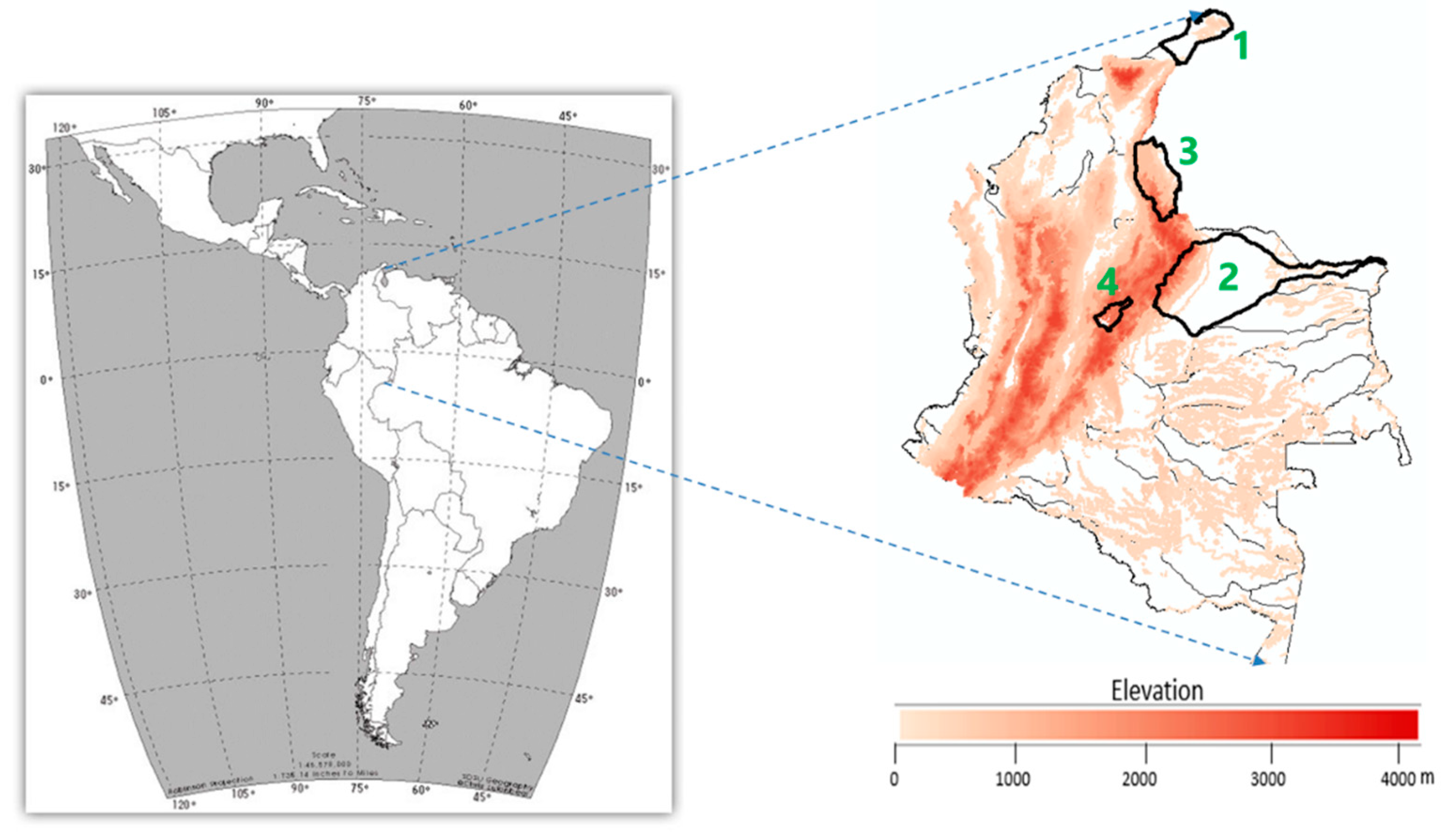
The areas analyzed in this study comprises four representative areas characterized as individual water sectors on the east side and in the middle of Colombia with different geographic and climatic conditions. These regions lie between 74°56′13″ and 66°82′29″ west longitude, and between 12°24′40″ north and 2°18′25″ south latitudes. These regions are named Alta Guajira, Bajo Meta, Rio Catatumbo and Sabana de Bogota. They were selected due to each region’s variability of conditions and the sufficient availability of data for analysis.
Colombia is located in the northwestern corner of South America, exhibiting complex geographical, environmental, and hydroecological features. Colombia is crossed by three rugged parallel ranges of the Andes Mountains—namely, the Eastern, Central, and Western Cordilleras. Precipitation along the country is highly influenced by the Inter Tropical Convergence Zone (ITCZ); however, the climate is also conditioned by local particularities like those caused by mountain barriers to the atmospheric circulation. On seasonal time scales, the displacement of the ITCZ exerts a strong control on the annual cycle of Colombia’s hydroclimatology [14,15,16]. Some regions of the country experience a bimodal annual cycle of precipitation with distinct rainy seasons and dry seasons, while others experience a unimodal annual cycle, which result from the different passages of the ITCZ over those regions. Moisture transported from the Amazon basin encounters the orographic barrier of the Andes, thus, focusing and enhancing deep convection and rainfall in the eastern flank of the Cordillera, with the maximum rainfall occurring during June–August. The interannual variability of the diurnal cycle is dominated by the effects of both phases of El Niño Southern Oscillation (ENSO).
The east side of Colombia is hot in most of its extension, with a range of medium temperature from 12 to 34 °C. The eastern side of the country borders Venezuela, the Amazon is to the south, extensive valleys and the Andean mountains are on the mid-eastern side, and coastal plains towards the higher north. These plains are tropical grasslands that undergo seasonal flooding; they are suitable for livestock grazing and in some areas for the cultivation of crops. Additionally, major petroleum discoveries have been made in the eastern region.
3. Materials and Methods
3.1. Meteorological Data
Historical daily data of precipitation, maximum temperature, minimum temperature, and relative humidity from 153 hydrometeorological stations along the four studied regions was provided by the Institute of Hydrology, Meteorology and Environmental Studies of Colombia (IDEAM). From this, only datasets with less than 30% of missing values for the time range of 1980–2015 were considered for the analysis. This was used in concordance with the minimum extension of 30 year-records, which is recommended by the World Meteorological Organization [17] in order to obtain reliable statistics. Figure 1 and Table 1 show the location and description of the 4 analyzed regions or water districts; the climate characterization refers to Lang’s Index (I = Pr/Tm), where Pr is the mean annual precipitation amount and Tm is the mean annual temperature. In some of these water districts, several climate conditions coexist.
Projected daily data sets for the same variables and for the future periods 2021–2050 and 2071–2100 were created from a regional downscaling procedure [18], using the statistical downscaling model SDSM and datasets from two Global Climate Models (GCM), which are part of the CMIP5-project, the Global Climate Model CanESM2 developed by Canadian Centre for Climate Modelling and Analysis and the model IPSL-CM5A-MR developed by The Institut Pierre Simon Laplace. Both GCM included in the study (as most GCM used to date) used fundamental physical laws, which were then subjected to physical approximations like equations of Geophysical Fluid-Dynamics that are appropriate for describing the atmosphere and the ocean at large enough scales. The Representative Concentration Pathways—RCP 2.6 and RCP 8.5 were considered for both models, representing two different possible future emission trajectories and radiative forcings. The RCP 8.5 combines assumptions about high population and relatively slow income growth with modest rates of technological change and energy intensity improvements, leading to a high energy demands and greenhouse gas (GHG) emissions in the long term, in the absence of climate change policies. The RCP 2.6 might be described as the best case for limiting anthropogenic climate change. In this scenario, Global CO2 emissions peak by 2020 and decline to around zero by 2080. The concentrations in the atmosphere peak at around 440 ppm in midcentury and then slowly start declining.
3.2. Soil and Land Cover
The values of the different canopy and vegetation variables were taken from available local studies, and maps provided by IDEAM. Physical characteristics of the different types of soils for each region were obtained from regional studies in the areas. The overall available information about the general soil characteristics of the whole extension of the study sites was relatively low, most of the data used for the analysis corresponded to the maps provided by the IDEAM and the local authorities. Three of the studied regions, not including Alta guajira, were relatively similar in terms of soil properties but did show significant differences in terms of land cover. In these regions, numerous wetlands can be found along with some urban areas; however, grassland and tropical forest are the main land-cover types for all of regions, even though the portions differ.
3.3. Model
The model BROOK90 [19] was used in this study for the water balance assessment in the historical and the different projected scenarios. BROOK90 is a deterministic, process-oriented, lumped parameter hydrologic model that can be used to simulate the water balance in most land surfaces at a daily time-step, year-round. The model has a strong physically based description that simulates the above and below liquid phases of the precipitation–evaporation–streamflow–ground water flow part of the hydrological cycle for a point-scale stand at a daily time-step [20]. The BROOK90 model calculates evaporation through the Shuttleworth–Wallace approach [21], as well as an improvement of the Penman–Monteith equation. The characteristics of the soil water were determined using a modified approach of the Brooks and Corey [22], and Saxton et al. [23]. The water movement through the soil was simulated using the Darcy–Richards equation. To calculate streamflow, the model used a simplified process—storm flow by source area flow or subsurface pipe-flow and delayed flow, from vertical or downslope soil drainage and first-order groundwater storage. A general water balance equation can be represented as follows:
where PREC represents precipitation (mm), EVAPOT is the evapotranspiration (mm), FLOW is the corresponding simulated total streamflow (mm) derived from surface flow and groundwater flow, and STORAGE is the deep seepage loss from groundwater (mm). Applications of the BROOK90 model have been demonstrated in grasslands, temperate evergreen and deciduous forests [19], and cultivated lands [24], among various vegetations with satisfactory performance. The model is also applicable in the tropics after adjusting the parameters to local conditions.
PREC = EVAPOT + FLOW + STORAGE
3.4. Data-Grid and Interpolation
The study intends to show the change in water budget caused by climate change over the studied regions on a bigger scale than a watershed scale. For this reason, the study was focused primarily on water sectors that covered a much bigger extension of an area. This would give a wider overview and understanding of the availability of water for several cities and settlements located in and around these regions, as well as the productive activities developed in the area. With this purpose, the data from the stations (including historical and future data) were interpolated and converted into a 10 km × 10 km grid of datasets. This is an appropriate approach considering the irregular distribution of the stations and the highly variable geography of the areas. It further enables the possibility of conducting a water balance calculation in areas where no historical data are available, while also being located at different elevations from the station point. The data were interpolated using the Thin Plate Spline Method (TPS). This is a spline-based technique for data interpolation and smoothing and it has been proven to perform a good interpolation for precipitation data (Tait et al., 2006). For interpolation of scattered z(x,y) data, the TPS is just a special case of Radial Basis Function (RBF) interpolation:
where p(x,y) is a polynomial function and ϕ is an RBF. In the case of TPS, ϕ = r2 ln(r). The water balance would be calculated for each of the grid points using BROOK90 and all available data. The results for the baseline historical period of 1981–2010 would be compared with the results obtained for the different projected scenarios, considering the two Representative Concentration Pathways RCP 2.6 and RCP 8.5, the two GCM, and the two projected periods 2021–2050 and 2071–2100. The comparison would allow one to visualize the expected differences in the availability of water for the future decades, due to the effects of climate change.
4. Results
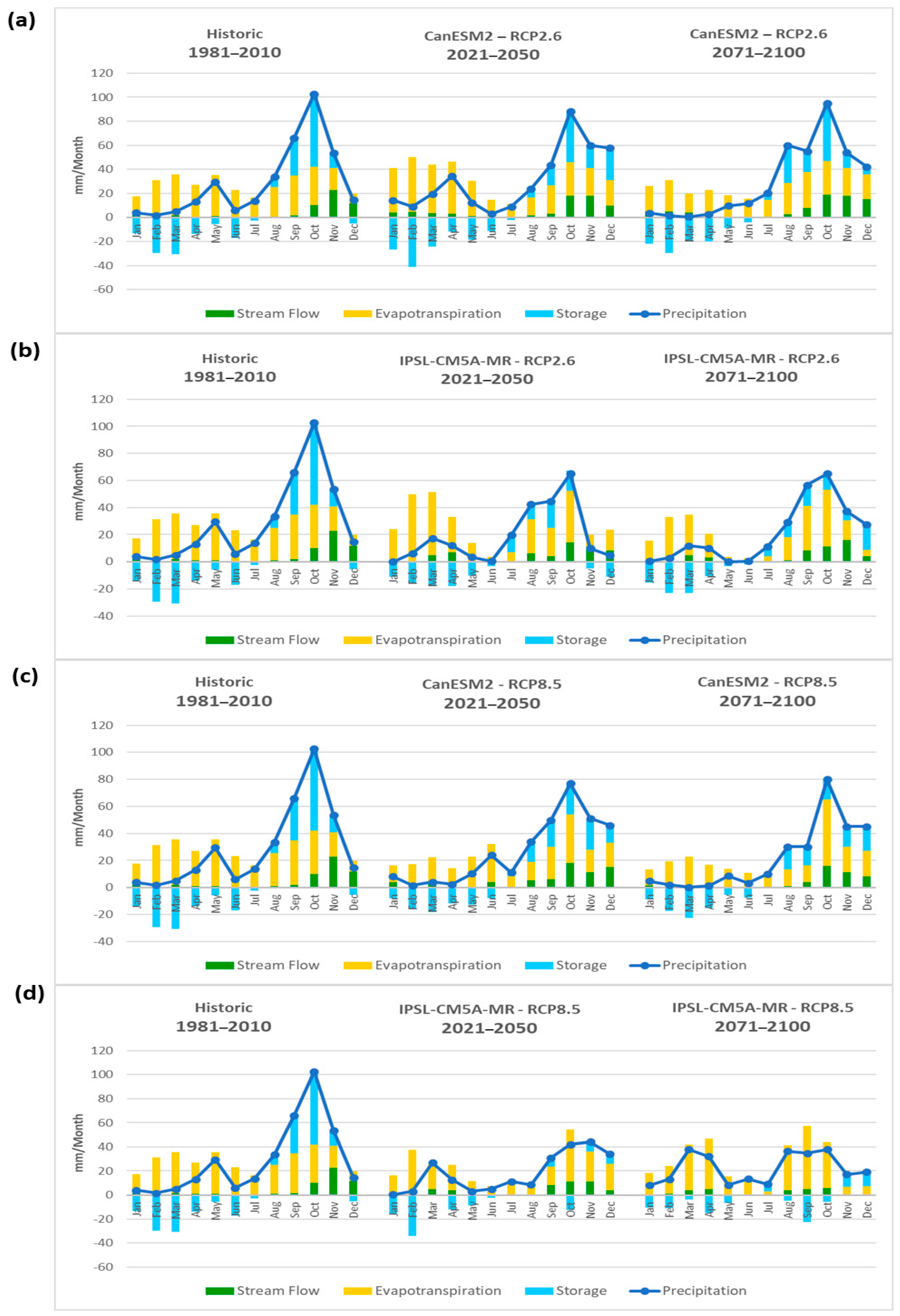
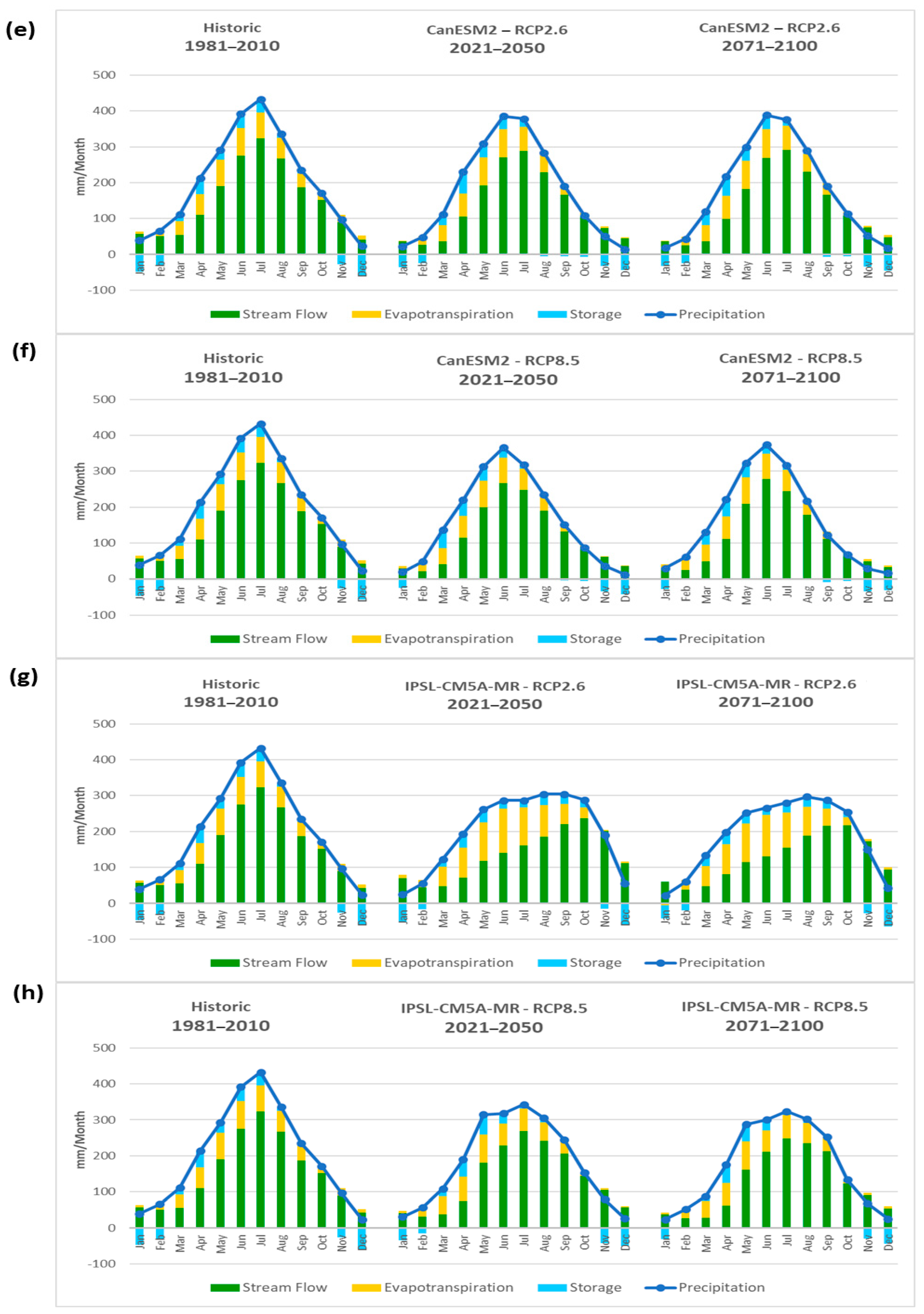
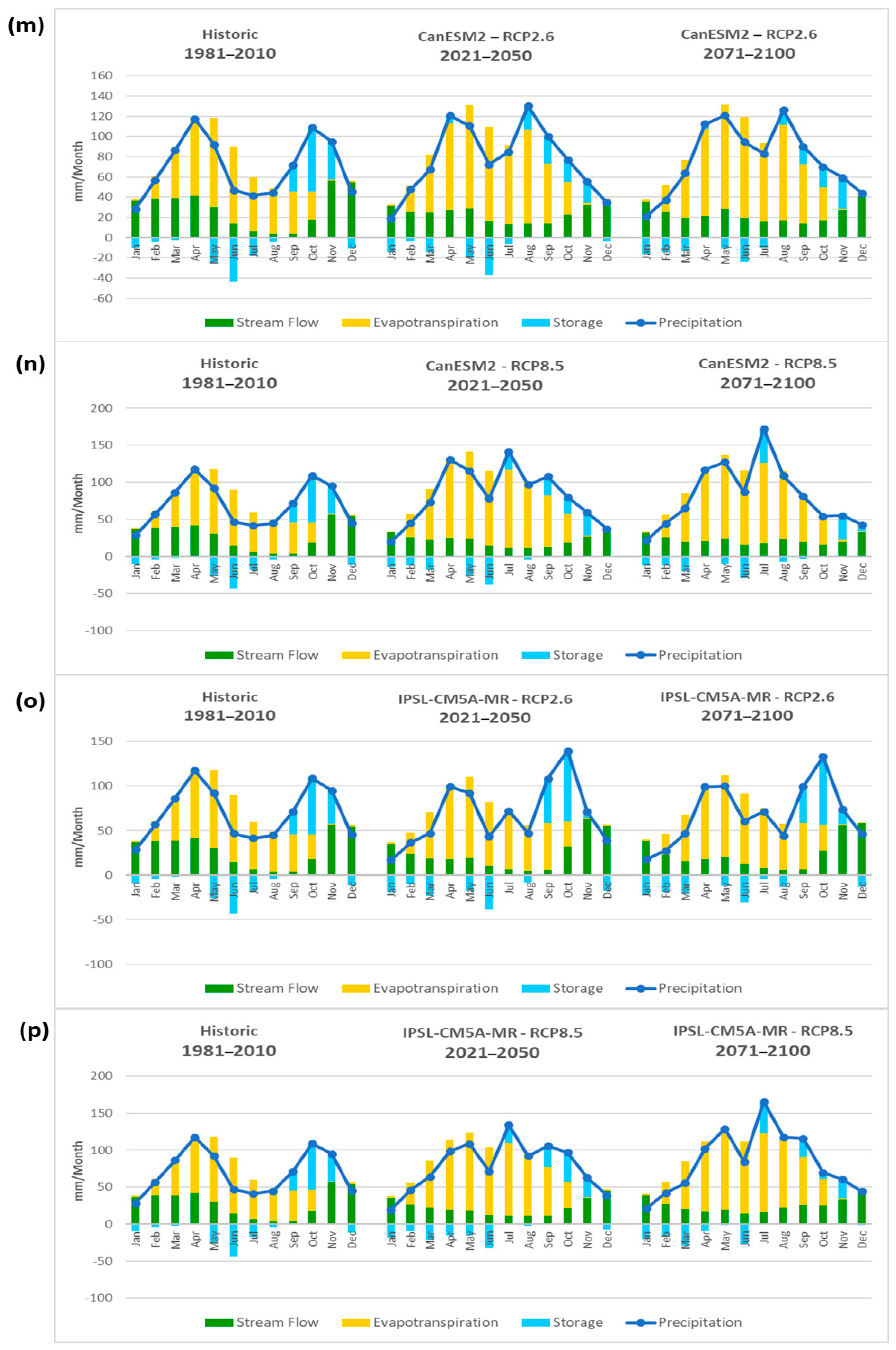
The graphs provided in Appendix A show an overview of monthly average results for the 4 studied areas. Here, one can compare the three periods of time (historical baseline 1981–2010, future projections 2021–2050, and 2071–2100) for each area, each GCM, and each Representative Concentration Pathway. As an example, in Figure A1a of Appendix A, the results for the three periods of time in the Alta Guajira region and the scenario with the model CanESM2 and Representative Concentration Pathway RCP 2.6 can be observed. The results are expressed in terms of the water balance components given by Equation (1). Table 2 shows the relative increment or decrease for each projected component of the water balance in the different climate scenarios, compared to the reference period of 1981–2010.
Projected soil moisture for the 4 studied regions as an averaged monthly value can be seen in Figure 2, the results for the climate scenarios are then compared with the baseline period of 1981–2010.
5. Discussion
In Appendix A and Appendix B, one can appreciate the notorious difference between the climate conditions and the water availability between the four studied regions, with regards to the historical period as well as to the projections. In general terms, the water balance components in the different regions showed different patterns magnitudes due to variability in precipitation along the Colombian territory. The region of Sabana de Bogota (Appendix A, m–p) showed a clear bimodal precipitation regime and the region Meta (Appendix A, e–h) showed a clear monomodal regime; the other two regions presented a not-so-clearly defined bimodal regime—these precipitation conditions were obedient to the displacement of the ITCZ over the regions.
The region of Alta Guajira being an arid/desert region shows very low levels of precipitation for most of the year. It reaches a peak of about 105 mm by the month of October, generates low levels of streamflow, since almost 85% of the total precipitation in the year is converted into evapotranspiration due to the high temperatures. In the first three months of the year, evapotranspiration can be almost 8 times larger than precipitation. During this time, the storage water produced as a consequence of the rainy season in the last months of the year is constantly being evaporated. The projections for Alta Guajira showed a decrease in precipitation, in general terms, and, therefore, a decrease in the other components of the water balance. This was the case for both projected periods of time of 2021–2050 and 2071–2100. Only the model CanESM2 with scenario RCP 2.6 showed a slight increment of precipitation in the short and long term.
From the four analyzed areas in this study, Bajo Meta presented the highest amount of rain on a yearly basis. In this region, the results showed an almost “normal” distribution of precipitation throughout the year for the historical records—presenting the highest values in the months of June and July with a peak of 430 mm/month and a non-rainy season at the end and beginning of the year. Most of the precipitation in Bajo Meta was converted into streamflow during the year (74.3%). This might be due to the characteristics of the soil (a predominant silty loam type for a big part of this region), which does not allow a big rate of infiltration. The projections for this region showed a decrease in precipitation, which led to a directly proportional decrease in streamflow; evaporation showed variable results depending on the model; CanESM2 indicated a slight decrease for both RCP scenarios, while IPSL-CM5A indicated the opposite. These results are reasonable considering that for the first model the decrease in precipitation was much bigger in magnitude than the second model.
The historical period indicates that in the region of Rio Catatumbo, half of the precipitation in the year was evaporated (50.7%) and a similar level was converted into streamflow (45.1%). In general terms, the projections for the future showed a slight decrease of the precipitation regimes, with around 6% from the model CanESM2 and around 9% from the model IPSL-CM5A but with a much higher decrease in the levels of streamflow produced by this precipitation. Evaporation in both models was projected to increase at levels of around 20% for the next decades. This was linked to the projected increase in the temperature for the region, which was close to 4 °C for the end of the century with the scenario RCP 8.5, according to the results from the regional downscaling procedure [18].
In the region of Sabana de Bogota, the historical period showed that 58% of the precipitation was evaporated while only 41% converted into streamflow. The typical clay type of soil predominant in a big part of the region was reflected in the low levels of stored water. Sabana de Bogota was the only one from the analyzed four regions where an increase of precipitation was projected for the next decades; Table 2 shows that the biggest increment was in the period of 2071–2100, with the model IPSL-CM5A and the scenario RCP 8.5. These projections showed that the levels of evaporation would increase in a considerable rate compared with the historical period. It was clear from Appendix A (m–p) that a bigger percentage of the projected precipitation would evaporate, compared with the historical baseline.
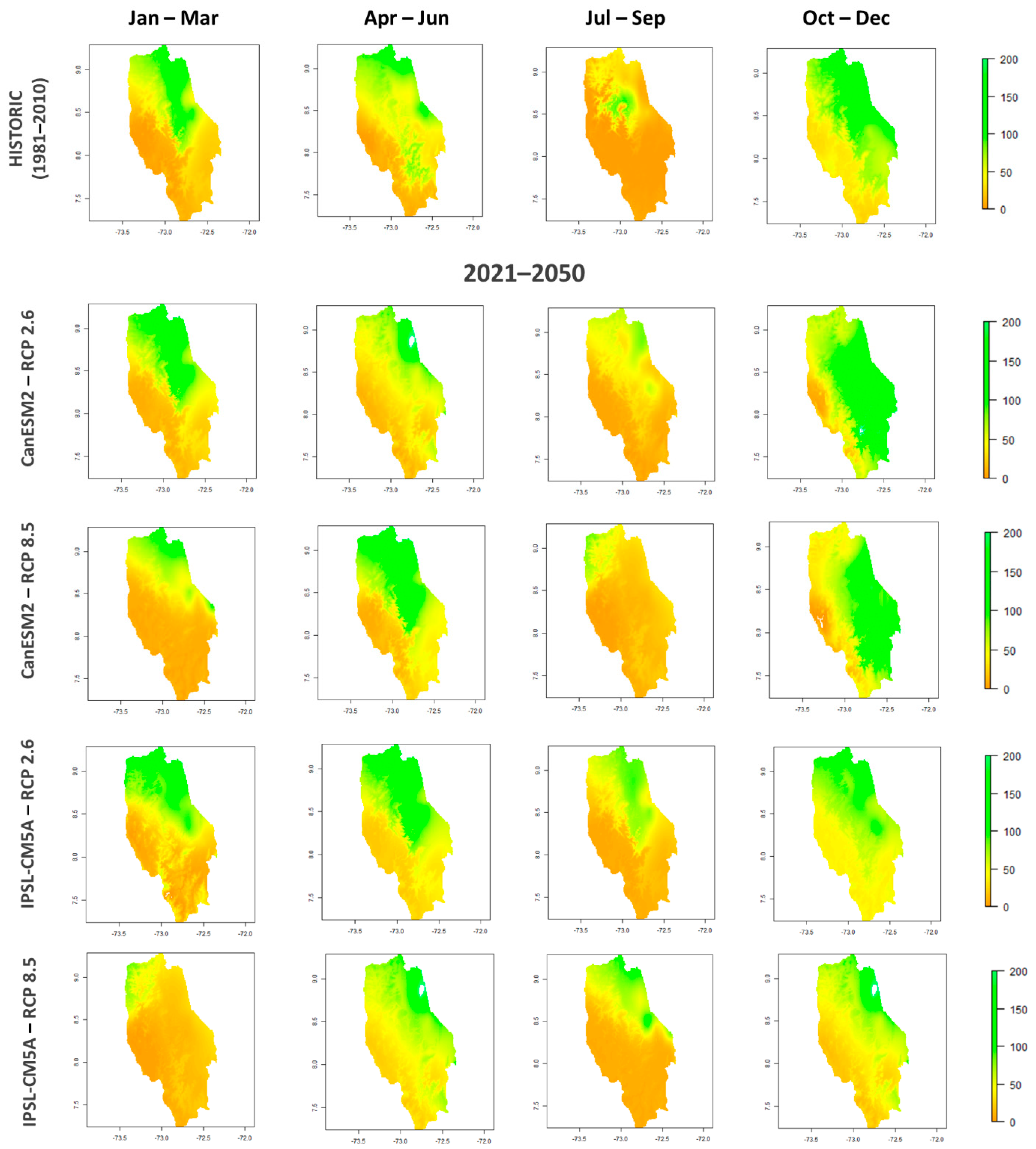
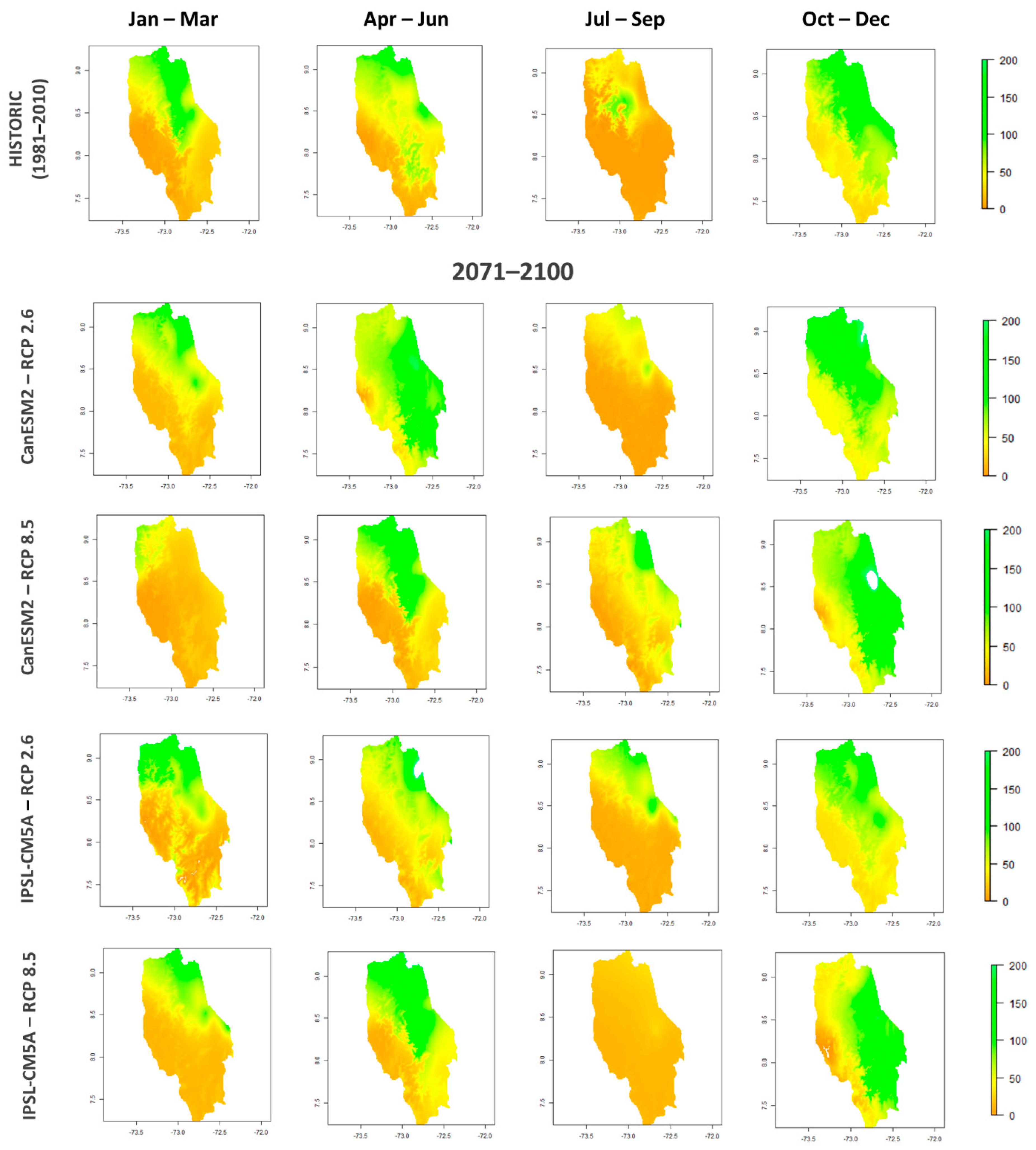
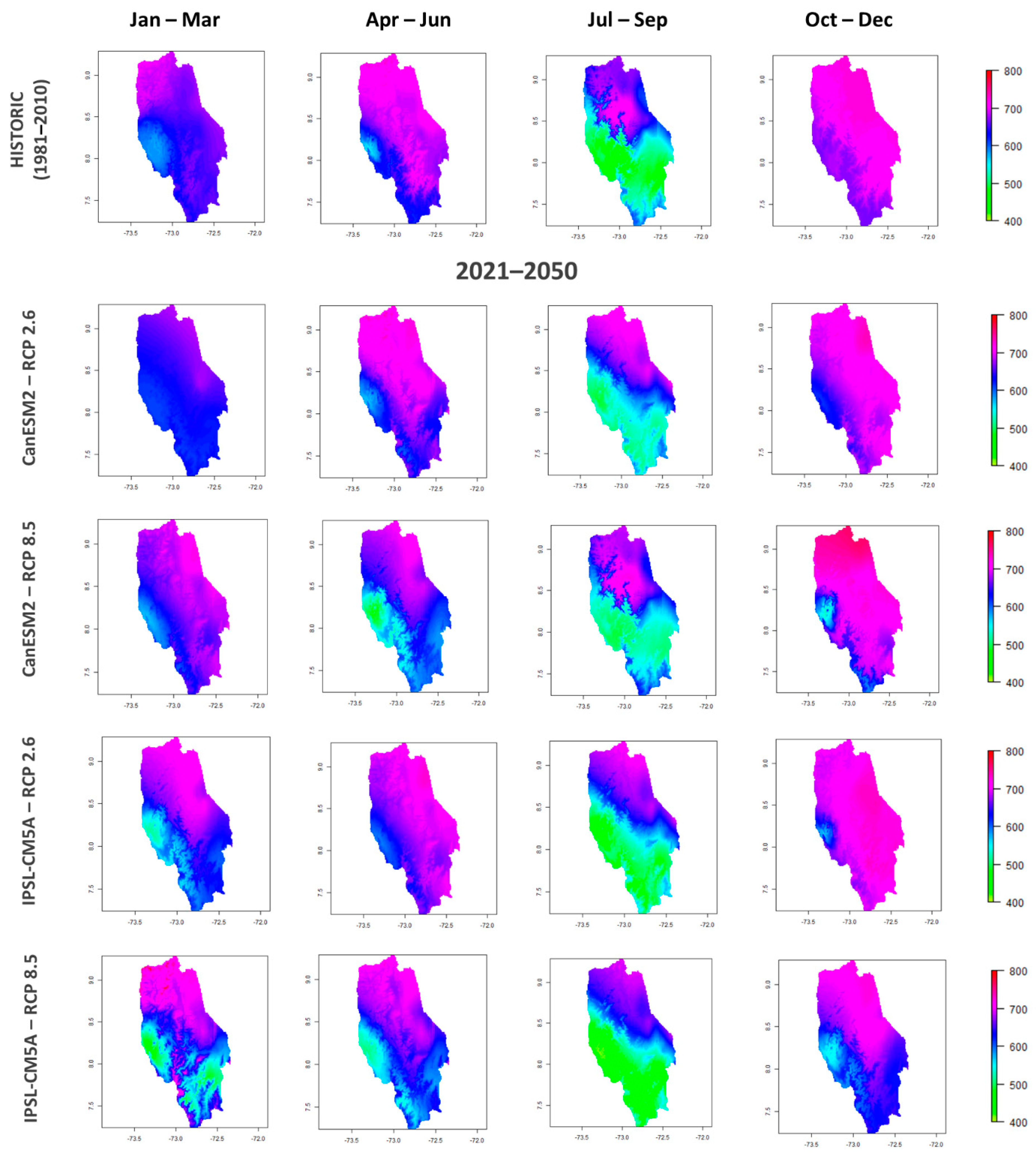
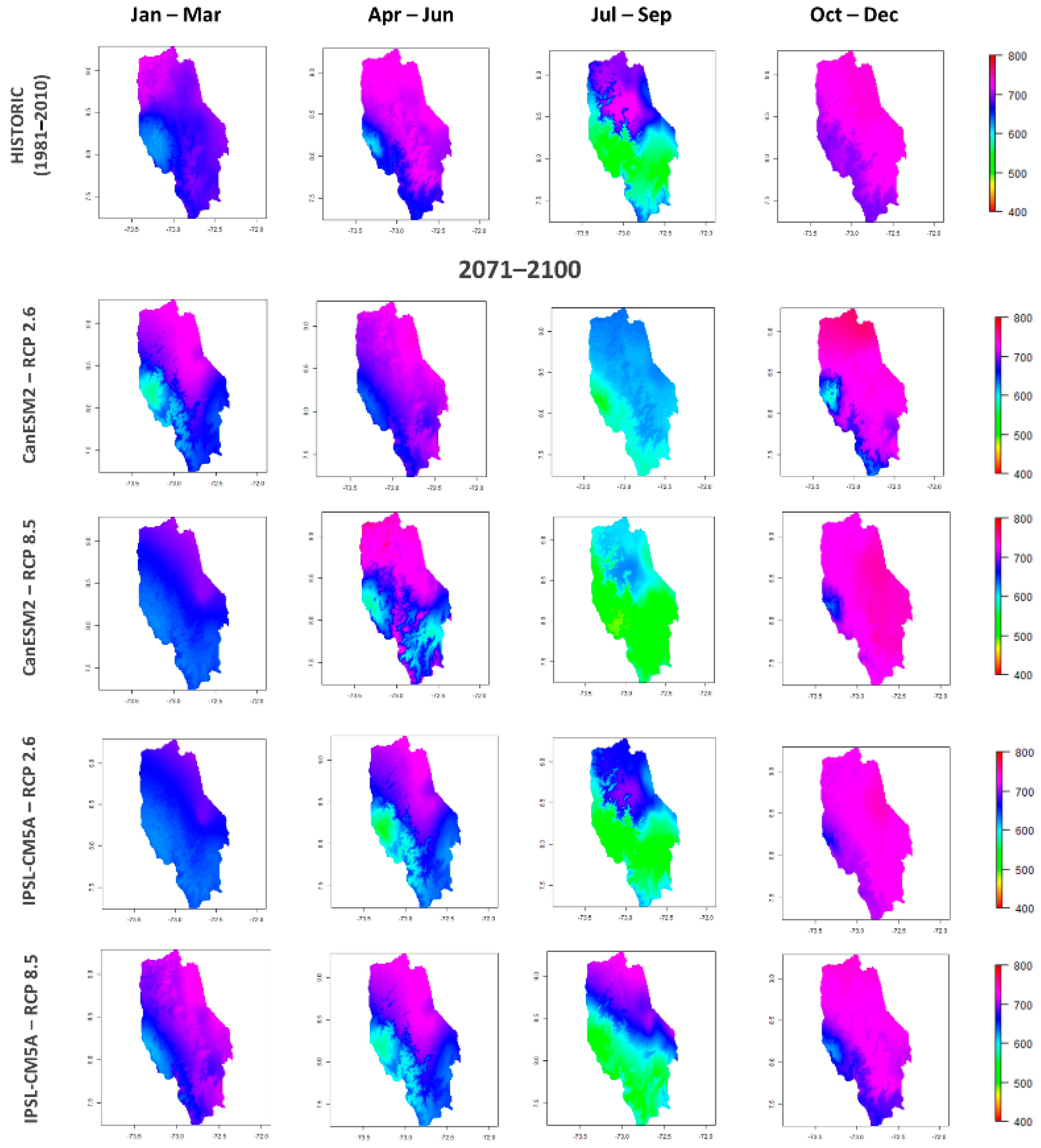
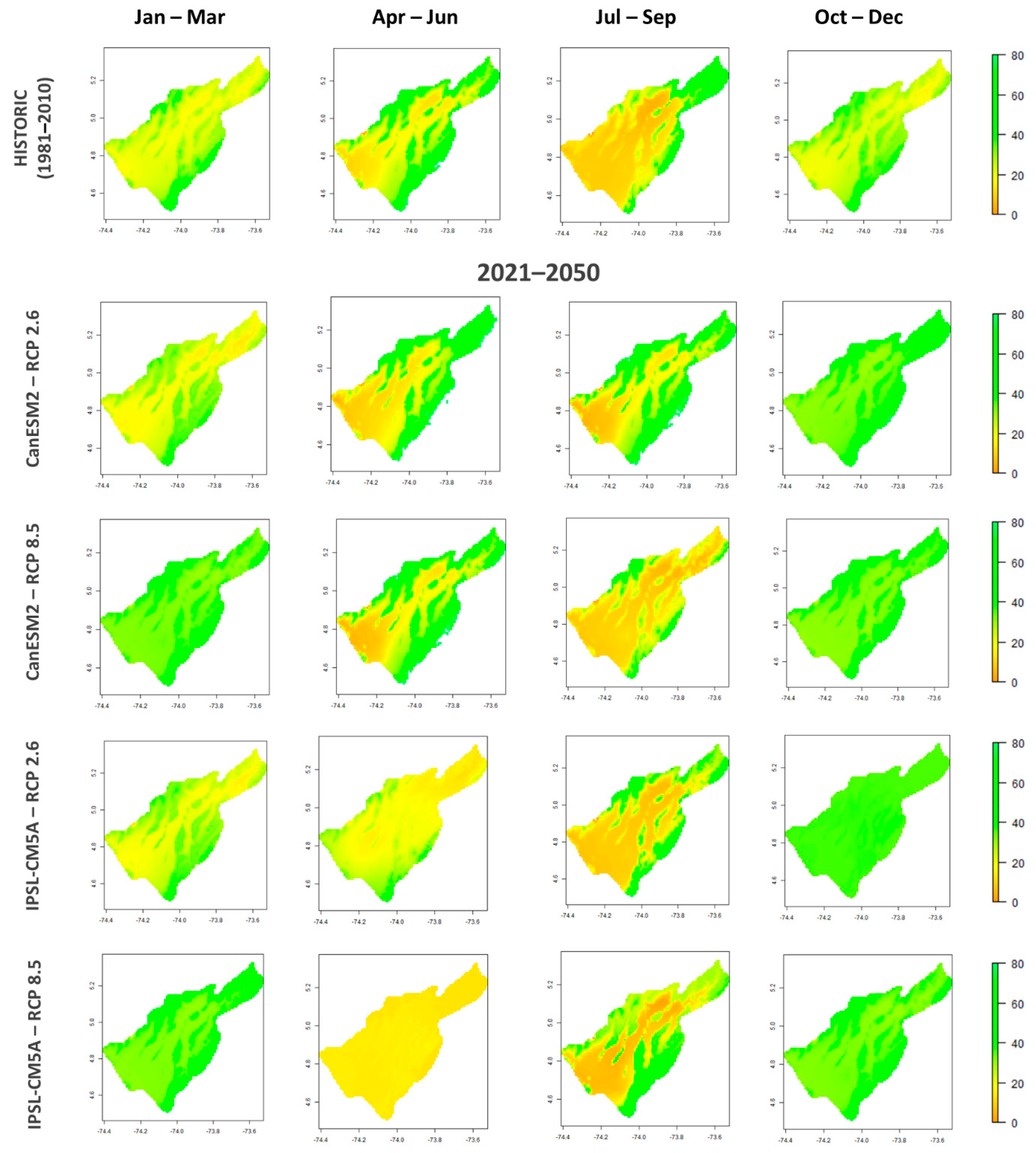
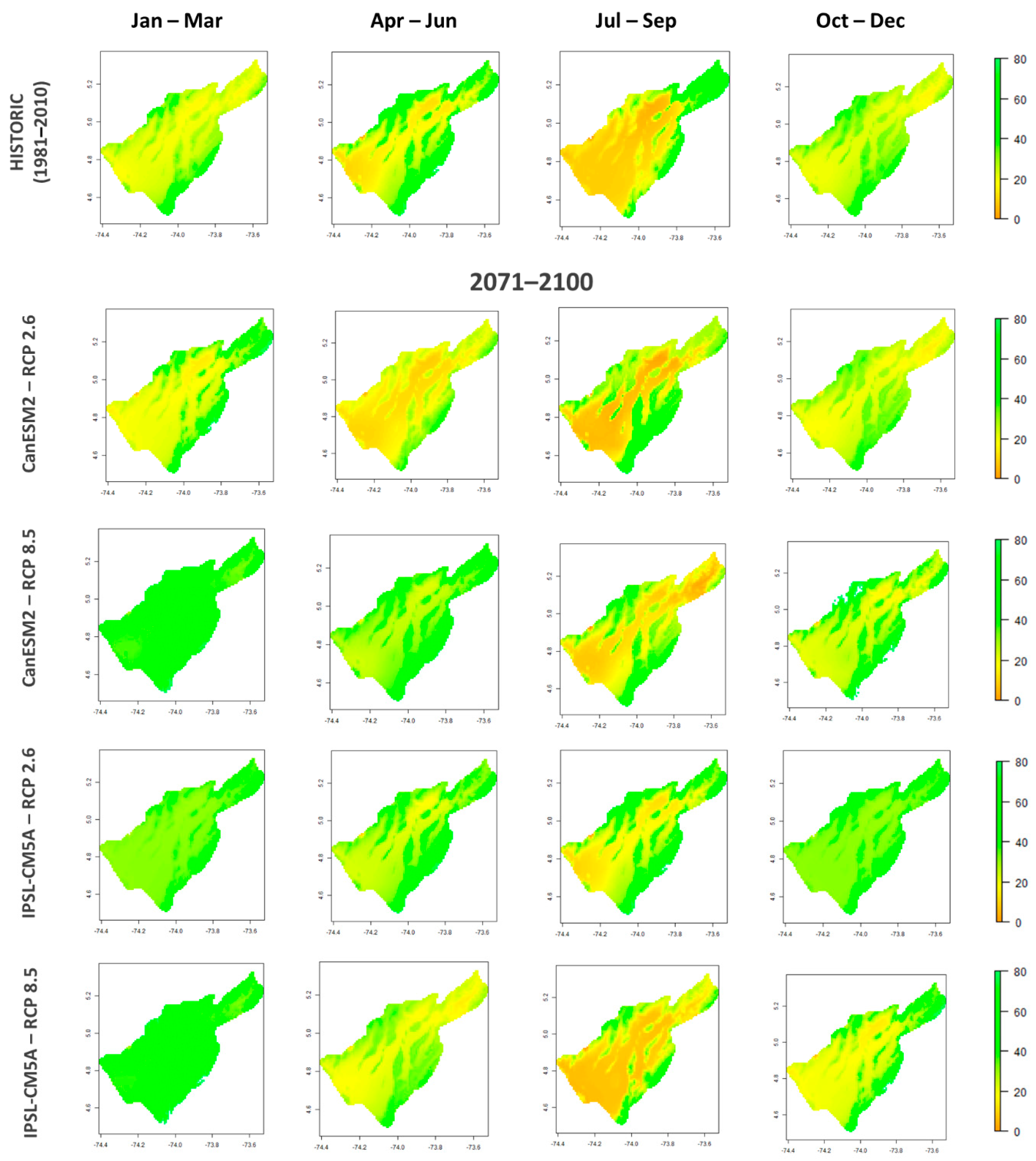
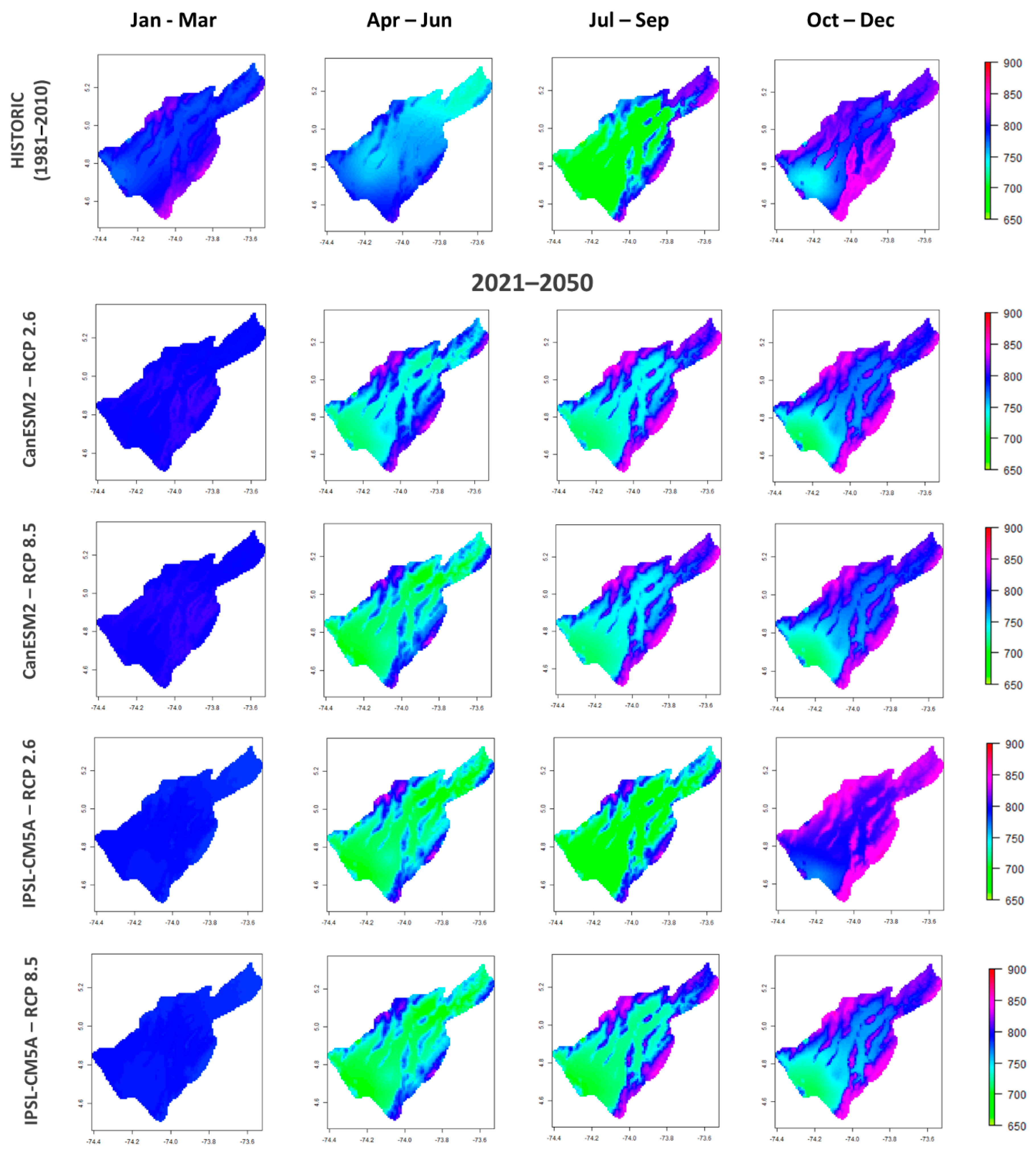
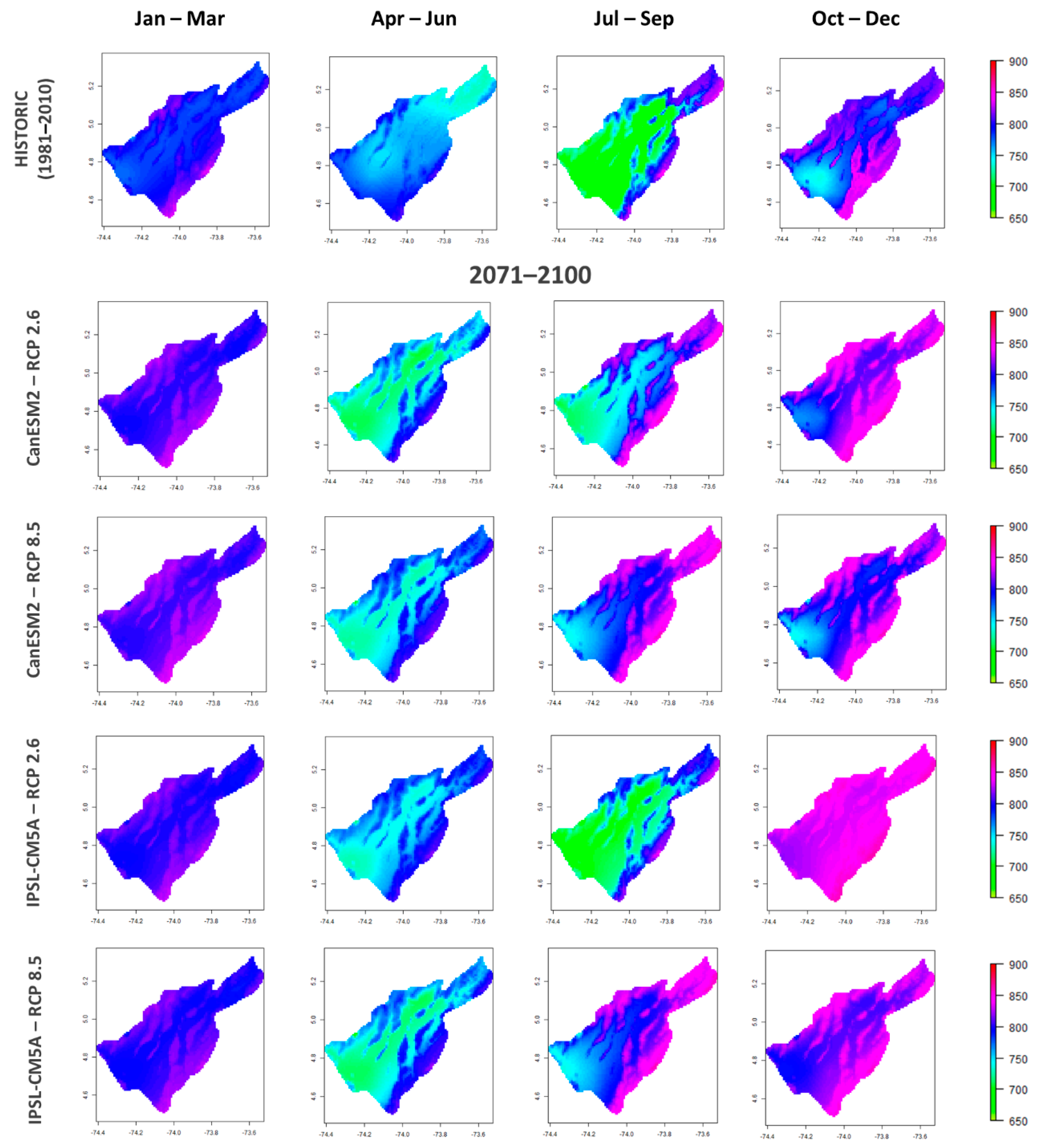
It is important to consider that the results obtained in this study and shown in Figure 2 and Appendix A are the averaged-out product of the results of each station in the region. This was made with the purpose of obtaining results in a macro-scale, to have a notion of the projected scenarios for water districts, where productive and social activities are planned in accordance with the available water in that area. An analysis for an individual station or an area of a much higher resolution could also show variable results, depending on the elevation of the studied area. The rasters produced in Appendix B are a useful representation of the spatial variability of the historical and projected results for two of the studied regions, when considering the geographical variation presented in each of them. As was said before, the spatial distribution density of meteorological stations at the other two regions was too low to allow a proper interpolation process to create a figure that reliably showed a representation of spatial variability of the results throughout the regions.
Figure 2 shows that, in general, soil moisture would be reduced considerably in the next decades, the percentage of decrease could vary for each scenario; the only exception was the region of Sabana de Bogota, where precipitation is projected to increase, which would result in an increase in the soil moisture. These results are important in relation to agricultural activities and the planning/use of soil for the next decades.
The lack of available historical records of discharge in the studied areas as well as the wide extent of these areas, made the performance of a respective process of calibration and validation of the water balance components that comprises all extensions of the studied areas unsuitable, however, an intensive review of the input data to the model was carried out to ensure an appropriate parameterization. This included a detailed selection of values regarding the information of soils in the studied areas, through technical information from the public and private sector. Information regarding vegetation comes mostly from Governmental institutes, as well as the detailed land use information that was also obtained from regional, territorial development plans. In the same way, a review of the results of the model and a comparison with results of other studies nearby, in tropical or similar areas was made [25,26,27,28,29,30,31], to verify the veracity of the results and ensure that they are within a correct range of magnitudes.
The main differences of both GCM that were used for a regional downscaling as a source of the projected climate data used in this study are their spatial resolution; CanESM2 with 2.79° latitude × 2.81° longitude and IPSL-CM5A-MR with 1.26° latitude × 2.5° longitude, as well as the model-components with which they were coupled; CanESM2 consists of a physical atmosphere–ocean model coupled to a terrestrial carbon model and an ocean carbon model, while the IPSL-CM5A-MR model couples four components of the Earth system, atmospheric dynamics and physics, ocean dynamics, sea ice dynamics and thermodynamics, and land surface. Moreover, every single GCM differs in the parametrization of the physical modeled processes, for this reason they offer varied results that might be more successfully correlated with real measurements in some areas than others. The model IPSL-CM5A, in spite of its slightly higher spatial resolution has shown a better performance than other models to identify extreme events in South America and other regions [32], but a lower performance to appropriately reproduce precipitation historical records in comparison with CanESM2 and other models, in Colombia and South America [33,34]. This agreed with the results of this study, where extreme events and seasonal precipitation was more clearly identifiable for the model IPSL-CM5A, especially in regions of lower elevations, where the model seemed to overestimate the projected change for the different variables.
Rainfall seasonality and its interannual variability have been observed to change in magnitude, timing, and duration, in the tropics [35]. As mentioned before, the climate in Colombia is conditioned by local particularities like those caused by mountain barriers to the atmospheric circulation but the annual cycle of Colombia’s hydroclimatology is mostly influenced by the displacement of the ITCZ. The different passages of the ITCZ over the regions determine either a bimodal annual cycle of precipitation with distinct rainy seasons and dry seasons, while others experience a unimodal annual cycle that result from the moisture transported from the Amazon basin when it encounters the orographic barrier of the Andes. The seasonality of hydrological elements in the different water districts shows larger variability due to their different conditions of topography, hydrogeology, and vegetation. Higher regions like Sabana de Bogota or parts of Rio Catatumbo are highly dependent on altitude, and since there is no snow formation in any of the regions, there is no considerable time lag between the precipitation event, the stream flow, and the soil moisture, which can be observed in Figure 2 and Appendix A. A prolonged positive soil humidity in the humid regions seen in Figure 2 linked directly with rain events explained by a permeable soil and temperature that was not high enough to increase evapotranspiration for several months. Climate seasonality is a defining feature of many ecosystems, often characterized in the tropics by a distinct non-uniformity in their timing of annual rainfall. This results in one or two wet seasons during which most of the annual rainfall occurs, separated by prolonged dry periods. In regions like Bajo Meta or Rio Catatumbo, under conditions of relative water abundance, long-term evapotranspiration becomes limited by the potential evapotranspiration, while in arid regions like Alta Guajira, where the energy supply is high, precipitation is the main constraint to evapotranspiration. In the former case, water supply exceeds demand, while in the latter case water supply is outstripped by the demand [36]. In Alta Guajira a projected increase in mean temperature would likely lead to increase in the frequency and the intensity of seasonal droughts [37].
It is important to consider that although the RCP 2.6 scenario might be described as the best case for limiting anthropogenic GHG emissions, their atmospheric concentrations will continue to increase even after emissions slow down and then will eventually start to decrease [38]. Carbon dioxide accumulates in the atmosphere and stays there for decades. Even if emissions start reducing in 2020, the concentration continues increasing and starts falling very slowly, only after 2050. This might explain why in some of the results of RCP 2.6 in Table 2, a bigger percentual change is observed for the period 2020–2050 than for the period of 2070–2100. However, as expected, the results obtained for the projections in the scenario RCP 8.5 showed a higher projected change than those in the scenario 2.6, this is the case for the analyzed regions except in Alta Guajira with model CanESM2, where the results showed a slight increase in precipitation under scenario 2.6, and a negative change under scenario 8.5 and model IPSL-CM5A_MR. This could have been caused by the incapacity of the model to accurately predict changes of precipitation in very arid areas that are characterized by little but highly variable and unpredictable rainfall and has been shown in other studies like Zhao [39] who analyzed the performance of the GCM models used in the CMIP5-project in several arid regions of the world, or by Mingxia [40] which found similar results across dryland areas.
The inherent existence of uncertainty in every water budget approach must be taken into consideration. Uncertainty related to hydrological modeling is affected by the input data, validation data, model structure, and model parameters. In order to reduce the uncertainties as much as possible in the hydrological modeling in this study, a detailed parametrization of the model was intended for each of the grids cells that the regions were divided into. For this, soil, vegetation, land use, and topography data were taken from local private studies and maps provided by governmental institutions and the parameters were individually defined for each of the cell grids where the model was run individually.
The hydro-climatic model chain typically consists of the components—emission scenario, GCM, regional climate model or statistical downscaling, and hydrological model [41]. This study represents the last step of that chain, but all of these components constitute a potential uncertainty source for the results. The uncertainty associated with the individual components of this chain has been investigated by an increasing number of studies. In some of them, the GCM structure is identified as the dominant source of uncertainty, e.g., [42,43,44]. A common finding for other studies is that in the hydrological model, uncertainty is less important than other sources but cannot be ignored [45,46,47]. Ideally, the analysis of hydrologic change in future studies should comprehend the full suite of uncertainties associated with global climate modeling, climate downscaling, hydrologic modeling, and natural climate variability. In this manner, the water resources planning and management community can make more informed decisions. Parameter uncertainty estimation is one of the major challenges in hydrological modeling and analysis of future change for the water sector is an interdisciplinary endeavor [48]. Ongoing parallel efforts to monitor and verify water budget components would help to improve accuracy. Posterior analysis could be done in an effort to determine the magnitude of the uncertainty of the hydrological response to climate change. Due to the uncertainties associated with the study of climate change and the limitations of models in representing climate and hydrological response, the most trustworthy indicator is still the trends observed at the measuring stations while the predictions of models in a big scale like that in this study might only be used to have a general notion of trends for the studied variables under different potential climate conditions.
The main objective of this study was to provide an overview of water budget response to climate change for a region where no other studies have been performed, and where not so much information was available since the few existing studies in Colombia have been aimed at regions with a bigger density of available data. In the analyzed regions in this study and especially in Alta Guajira and Bajo Meta, there is a lack of observed data with sufficient detail and quality. We encourage the future improvement of collection and testing of reliable data in a range of spatial and temporal scales in these regions, since it is critical to improve our understanding of hydrological processes [49].
6. Conclusions
The model BROOK90, historical data, as well as projected meteorological data were used to determine the changes in the water balance components in four different regions, which represent the four water districts in Eastern Colombia. The four regions reflect four different climatic and geographic conditions. The projected data were obtained from a statistical regional downscaling procedure, where two GCMs (CanESM2 and IPSL-CM5A-MR) and two different climate scenarios from RCP 2.6 and RCP 8.5 were used.
Results have shown a potential reduction in the generated streamflow for all studied regions. The temporal distribution of water balance components was considerably affected by the changing climate, which moreover, might have a profound impact on the hydrological regimes in these regions. Changes in evapotranspiration and stored water could vary from each region, according to the climate scenario, and the characteristics of soil and land use for each area. Results of spatial change of the water balance components have shown a direct link to the geography of each region and how the values differed accordingly, at different elevations. Soil moisture would be reduced considerably in the next decades and the percentage of decrease could vary for each scenario. Only in the region of Sabana de Bogota did the results show the opposite—this agreed with the precipitation projections that are to increase and, therefore, also the soil moisture.
Application of the model BROOK90 proved to be valuable for water cycle analysis and for the purpose of this study in offering a general overview to the change of water balance components, throughout the east side of Colombia, due to future climate change. Prediction of the impact of climate change on water budget components is a transcendent, practical, and theoretical problem to which each country and its institutions should dedicate more resources—especially for countries and regions that are more vulnerable to climate change.
Uncertainties associated with the GCMs, hydrological models, and the approaches used in this study have a direct effect on the outcome, and they have to be considered and evaluated for the use of these results, in addition to their uses for future works. The results obtained in this study should be considered as indicative of the expected trend in water resources of the studied regions, as a result of climate change. These results might serve as a baseline information for creating mitigating measures. However, future work using other models and other techniques for the analysis of water resources throughout these areas is encouraged.
Author Contributions
Conceptualization, methodology, software, analysis, writing, O.M.; Software, review, T.T.L.; Supervision, review and guidance, C.B. All authors have read and agreed to the published version of the manuscript.
Funding
This research received no external funding. The DAAD (German Academic Exchange Service) is the provider of the scholarship in which this research project took place.
Acknowledgments
We acknowledge the support given by the Open Access Publication Funds of the SLUB/TU Dresden. We thank IDEAM for providing the available historical records in the area.
Conflicts of Interest
The authors declare no conflict of interest.
Appendix A
Figure A1.
Alta Guajira.

Figure A2.
Bajo Meta.

Figure A3.
Rio Catatumbo.

Figure A4.
Sabana de Bogota.

Appendix B
Appendix B.1. Rio Catatumbo
Figure A5.
Stream Flow 2021–2050.

Figure A6.
Stream Flow 2071–2100.

Figure A7.
Soil Moisture 2021–2050.

Figure A8.
Soil Moisture 2071–2100.

Appendix B.2. Sabana de Bogota
Figure A9.
Stream Flow 2021–2050.

Figure A10.
Stream Flow 2071–2100.

Figure A11.
Soil Moisture 2021–2050.

Figure A12.
Soil Moisture 2071–2100.

References
- IPCC. Climate Change 2014: Synthesis Report. Contribution of Working Groups I, II and III to the Fifth Assessment Report of the Intergovernmental Panel on Climate Change; Pachauri, R.K., Meyer, L.A., Eds.; IPCC: Geneva, Switzerland, 2014; 151p. [Google Scholar]
- Band, L.; Mackay, D.; Creed, I.; Semkin, R.; Jeffries, D. Ecosystem processes at the watershed scale: Sensitivity to potential climate change. Limnol. Oceanogr. 1996, 5, 928–938. [Google Scholar] [CrossRef] [Green Version]
- Jimenez Cisneros, B.E.; Oki, T.; Arnell, N.W.; Benito, G.; Cogley, J.G.; Döll, P.; Jiang, T.; Mwakalila, S.S. Impacts, Adaptation and Vulnerability. Part A: Global and Sectorial Aspects. Contribution of Working Group II to the Fifth Assessment Report of the Intergovernmental Panel on Climate Change 2014; Cambridge University Press: Cambridge, UK, 2014; pp. 229–269. [Google Scholar]
- Healy, R.W.; Winter, T.C.; LaBaugh, J.W.; Franke, O.L. Water Budgets: Foundations for Effective Water-Resources and Environmental Management; U.S. Geological Survey Circular: Reston, VA, USA, 2007; Volume 1308, 90p.
- Burns, D.A.; Klaus, J.; McHale, M.R. Recent climate trends and implications for water resources in the Catskill Mountain region, New York, USA. J. Hydrol. 2007, 336, 155–170. [Google Scholar] [CrossRef]
- Candela, L.; Elorza, F.J.; Jiménez-Martínez, J.; von Igel, W. Global change and agricultural management options for groundwater sustainability. Comput. Electron. Agric. 2012, 86, 120–130. [Google Scholar] [CrossRef]
- Hagg, W.; Braun, L.N.; Kuhn, M.; Nesgaard, T.I. Modelling of hydrological response to climate change in glacierized Central Asian catchments. J. Hydrol. 2007, 332, 40–53. [Google Scholar] [CrossRef] [Green Version]
- Ruth, M.; Coelho, D. Understanding and managing the complexity of urban systems under climate change. Clim. Policy 2007, 7, 317–336. [Google Scholar] [CrossRef]
- Werritty, A. Living with uncertainty: Climate change, river flows and water resource management in Scotland. Sci. Total Environ. 2002, 294, 29–40. [Google Scholar] [CrossRef]
- Bates, B.C.; Kundzewicz, Z.W.; Wu, S.; Palutikof, J.P. (Eds.) Climate Change and Water; Technical Paper; Interguvernmental Panel on Climate Change: Geneva, Switzerland, 2008; 210p. [Google Scholar]
- Fu, G.; Charles, S.P.; Yu, J. A critical overview of pan evaporation trends over the last 50 years. Clim. Chang. 2009, 97, 193–214. [Google Scholar] [CrossRef]
- Miralles, D.G.; Holmes, T.R.H.; de Jeu, R.A.M.; Gash, J.H.; Meesters, A.G.C.A.; Dolman, A.J. Global land-surface evaporation estimated from satellite-based observations. Hydrol. Earth Syst. Sci. 2011, 15, 453–469. [Google Scholar] [CrossRef] [Green Version]
- IDEAM; PNUD; MADS; CANCILLERÍA; DNP. New Climate Change Scenarios for Colombia 2011–2100. Scientific Tools for National-Regional Level Decision-Making. Available online: http://documentacion.ideam.gov.co/openbiblio/bvirtual/022964/documento_nacional_departamental.pdf (accessed on 11 September 2019).
- Snow, J.W. The Climate of Northern South America. Climates of Central and South America; Schwerdtfeger, W., Ed.; Elsevier: Amsterdam, The Netherlands, 1976; pp. 295–403. [Google Scholar]
- Mejía, J.F.; Mesa, O.J.; Poveda, G.; Vélez, J.I.; Hoyos, C.D.; Mantilla, R.; Barco, J.; Cuartas, A.; Montoya, M.; Botero, B. Spatial distribution, annual and semi-annual cycles of precipitation in Colombia. DYNA 1999, 127, 7–26. (In Spanish) [Google Scholar]
- León, G.E.; Zea, J.A.; Eslava, J.A. General circulation and the intertropical convergence zone in Colombia. Meteor. Colomb. 2000, 1, 31–38. (In Spanish) [Google Scholar]
- WMO. WMO Guidelines on the Calculation of Climate Normals; WMO-No. 1203; Chairperson, Publications Board: Geneva, Switzerland, 2017; Available online: https://library.wmo.int/doc_num.php?explnum_id=4166 (accessed on 21 June 2019).
- Molina, O.D.; Bernhofer, C. Projected climate changes in four different regions in Colombia. Environ. Syst. Res. 2019, 8, 33. [Google Scholar] [CrossRef]
- Federer, C.A. BROOK 90: A Simulation Model for Evaporation, Soil Water, and Streamflow. 2002. Available online: http://www.ecoshift.net/brook/brook90.htm (accessed on 21 June 2019).
- Combalicer, E.A.; Lee, S.H.; Ahn, S.; Kim, D.Y.; Im, S. Modeling water balance for the small-forested watershed in Korea. KSCE J. Civ. Eng. 2008, 12, 339–348. [Google Scholar] [CrossRef]
- Shuttleworth, W.J.; Wallace, J.S. Evaporation from sparse crops—An energy combination theory. Q. J. R. Meteorol. Soc. 1985, 111, 839–855. [Google Scholar] [CrossRef]
- Brooks, R.H.; Corey, A.T. Hydraulic properties of porous media. Hydrol. Pap. 1964, 3, 1–27. [Google Scholar]
- Saxton, K.E.; Rawls, W.J.; Romberger, J.S.; Papendick, R.I. Estimating generalized soil water characteristics from texture. Trans. Am. Soc. Agric. Eng. 1986, 50, 1031–1035. [Google Scholar] [CrossRef]
- Wahren, A.; Schwärzel, K.; Feger, K.H.; Münch, A.; Dittrich, I. Identification and model based assessment of the potential water retention caused by land-use changes. Adv. Geosci. Eur. Geosci. Union 2007, 11, 49–56. [Google Scholar] [CrossRef] [Green Version]
- Bastidas Osejo, B.; Betancur Vargas, T.; Alejandro Martinez, J. Spatial distribution of precipitation and evapotranspiration estimates from Worldclim and Chelsa datasets: Improving long-term water balance at the watershed-scale in the Urabá region of Colombia. Int. J. Sustain. Dev. Plan. 2019, 14, 105–117. [Google Scholar] [CrossRef]
- Leta, O.T.; El-Kadi, A.I.; Dulai, H.; Ghazal, K.A. Assessment of climate change impacts on water balance components of Heeia watershed in Hawaii. J. Hydrol. Reg. Stud. 2016, 8, 182–197. [Google Scholar] [CrossRef] [Green Version]
- Louzada, F.L.R.; de, O.; Xavier, A.C.; Pezzopane, J.E.M. Climatological water balance with data estimated by tropical rainfall measuring mission for the Doce river basin. Eng. Agric. 2018, 38, 376–386. [Google Scholar] [CrossRef]
- Silva, A.L.; Roveratti, R.; Reichardt, K.; Bacchi, O.O.; Timm, L.C.; Bruno, I.P.; Oliveira, J.C.; Dourado Neto, D. Variability of water balance components in a coffee crop in Brazil. Sci. Agric. 2006, 63, 105–114. [Google Scholar] [CrossRef]
- Almeida, A.Q.; Ribeiro, A.; Leite, F.P.; Souza, R.; Gonzaga, M.S.; Santos, W.A. Water Balance in a Tropical Eucalyptus plantations in the Doce River Basin, Eastern Brazil. JAS J. Agric. Sci. 2019, 11, 209–217. [Google Scholar] [CrossRef]
- Schwerdtfeger, J.; Weiler, M.; Johnson, M.S.; Couto, E.G. Estimating water balance components of tropical wetland lakes in the Pantanal dry season, Brazil. Hydrol. Sci. J. 2014, 59, 2158–2172. [Google Scholar] [CrossRef] [Green Version]
- Escurra, J.J.; Vazquez, V.; Cestti, R.; De Nys, E.; Srinivasan, R. Climate change impact on countrywide water balance in Bolivia. Reg. Environ. Chang. 2014, 14, 727–742. [Google Scholar] [CrossRef]
- McSweeney, C.F.; Jones, R.G.; Lee, R.W.; Rowell, D.P. Selecting CMIP5 GCMs for downscaling over multiple regions. Clim. Dyn. 2015, 44, 3237. [Google Scholar] [CrossRef] [Green Version]
- Bonilla-Ovallos, C.A.; Mesa, O.J. Validación de la precipitación estimada por modelos climáticos acoplados del proyecto de intercomparación CMIP5 en Colombia. Rev. De La Acad. Colomb. De Cienc. Exactas Físicas Y Nat. 2017, 41, 107. [Google Scholar] [CrossRef] [Green Version]
- Yin, L.; Fu, R.; Shevliakova, E.; Dickinson, R.; Dickinson, R.E. How well can CMIP5 simulate precipitation and its controlling processes over tropical South America? Clim. Dyn. 2012, 41, 3127–3143. [Google Scholar] [CrossRef] [Green Version]
- Feng, X.; Porporato, A.; Rodriguez-Iturbe, I. Changes in rainfall seasonality in the tropics. Nat. Clim. Chang. 2013, 3, 811–815. [Google Scholar] [CrossRef]
- Feng, X.; Vico, G.; Porporato, A. On the effects of seasonality on soil water balance and plant growth. Water Resour. Res. 2012, 48, W05543. [Google Scholar] [CrossRef]
- Hartmann, D.L.; Tank, A.M.; Rusticucci, M.; Alexander, L.V.; Brönnimann, S.; Charabi, Y.A.; Dentener, F.J.; Dlugokencky, E.J.; Easterling, D.R.; Kaplan, A.; et al. Observations: Atmosphere and surface. In Climate Change 2013: The Physical Science Bases. Contribution of Working Group I to the Fifth Assessment Report of the Intergovernmental Panel on Climate Change; Stocker, T.F., Ed.; Cambridge University Press: Cambridge, UK, 2013; pp. 159–254. Available online: http://www.climatechange2013.org/report/full-report/ (accessed on 7 August 2019).
- MacDougall, A.H.; Eby, M.; Weaver, A.J. If anthropogenic CO2 emissions cease, will atmospheric CO2 concentration continue to increase? J. Clim. 2013, 26, 9563–9576. [Google Scholar] [CrossRef]
- Zhao, T.; Chen, L.; Ma, Z. Simulation of historical and projected climate change in arid and semiarid areas by CMIP5 models. Chin. Sci. Bull. 2014, 59, 412–429. [Google Scholar] [CrossRef]
- Ji, M.; Huang, J.; Xie, Y.; Liu, J. Comparison of dryland climate change in observations and CMIP5 simulations. Adv. Atmos. Sci. 2015, 32, 1565–1574. [Google Scholar] [CrossRef]
- Muerth, M.J.; St-Denis, G.; Ricard, B.; Velázquez, S.; Schmid, J.A.; Minville, M.; Caya, D.; Chaumont, D.; Ludwig, R.; Turcotte, R. On the need for bias correction in regional climate scenarios to assess climate change impacts on river runoff. Hydrol. Earth Syst. Sci. 2013, 17, 1189–1204. [Google Scholar] [CrossRef] [Green Version]
- Prudhomme, C.; Davies, H. Assessing uncertainties in climate change impact analyses on the river flow regimes in the UK. Part 2: Future climate. Clim. Chang. 2009, 93, 197–222. [Google Scholar] [CrossRef]
- Hagemann, S.; Chen, C.; Haerter, J.O.; Heinke, J.; Gerten, D.; Piani, C. Impact of a statistical bias correction on the projected hydrological changes obtained from three GCMs and two hydrology models. J. Hydrometeorol. 2011, 12, 556–578. [Google Scholar] [CrossRef]
- Dobler, C.; Hagemann, S.; Wilby, R.L.; Stötter, J. Quantifying different sources of uncertainty in hydrological projections in an Alpine watershed, Hydrol. Earth Syst. Sci. 2012, 16, 4343–4360. [Google Scholar] [CrossRef] [Green Version]
- Thompson, J.R.; Green, A.J.; Kingston, D.G.; Gosling, S.N. Assessment of uncertainty in river flow projections for the Mekong River using multiple GCMs and hydrological models. J. Hydrol. 2013, 486, 1–30. [Google Scholar] [CrossRef]
- Velázquez, J.A.; Schmid, J.; Ricard, S.; Muerth, M.J.; Gauvin St- Denis, B.; Minville, M.; Chaumont, D.; Caya, D.; Ludwig, R.; Turcotte, R. An ensemble approach to assess hydrological models’ contribution to uncertainties in the analysis of climate change impact on water resources. Hydrol. Earth Syst. Sci. 2013, 17, 565–578. [Google Scholar] [CrossRef] [Green Version]
- Jobst, A.M.; Kingston, D.G.; Cullen, N.J.; Schmid, J. Intercomparison of different uncertainty sources in hydrological climate change projections for an alpine catchment (upper Clutha River, New Zealand). Hydrol. Earth Syst. Sci. 2018, 22, 3125–3142. [Google Scholar] [CrossRef] [Green Version]
- Clark, M.P.; Wilby, R.L.; Gutmann, E.D.; Vano, J.A.; Gangopadhyay, S.; Wood, A.W.; Fowler, H.J.; Prudhomme, C.; Arnold, J.R.; Brekke, L.D. Characterizing uncertainty of the hydrologic impacts of climate change. Clim. Chang. Rep. 2016, 2, 55–64. [Google Scholar] [CrossRef] [Green Version]
- Xu, C.; Widén, E.; Halldin, S. Modelling hydrological consequences of climate change—Progress and challenges. Adv. Atmos. Sci. 2005, 22, 789–797. [Google Scholar] [CrossRef]
Figure 1.
Location of the studied areas with elevation.

Figure 2.
Monthly averaged soil moisture in (a) Alta Guajira; (b) Bajo Meta; (c) Rio Catatumbo; (d) Sabana de Bogota.
Figure 2.
Monthly averaged soil moisture in (a) Alta Guajira; (b) Bajo Meta; (c) Rio Catatumbo; (d) Sabana de Bogota.


Table 1.
Characteristics of the four analyzed regions.
| Region/Water District | Climate | Area (km2) | N° of Stations (Precipitation) | Min. Elevation (m.a.s.l.) | Max. Elevation (m.a.s.l.) | |
|---|---|---|---|---|---|---|
| 1 | Alta Guajira | arid, desertic | 12,348 | 25 | 1 | 390 |
| 2 | Bajo meta | semihumid | 42,655 | 42 | 45 | 3520 |
| 3 | Rio Catatumbo | humid | 17,960 | 47 | 83 | 1740 |
| 4 | Sabana de Bogota | semihumid, semiarid | 2245 | 39 | 2540 | 3800 |
Table 2.
Percentual change of the water-balance components in the projected scenarios.
| Precipitation (mm) | Streamflow (mm) | Evapotranspiration (mm) | Storage (mm) | |||||
|---|---|---|---|---|---|---|---|---|
| 2021–2050 | 2071–2100 | 2021–2050 | 2071–2100 | 2021–2050 | 2071–2100 | 2021–2050 | 2071–2100 | |
| Alta Guajira | ||||||||
| CanESM2 (RCP 2.6) | 9.12 | 3.68 | 17.73 | 35.07 | 13.73 | −10.36 | −22.34 | −21.03 |
| CanESM2 (RCP 8.5) | −0.88 | −24.15 | 66 | −22.75 | −22.24 | −26.74 | −44.64 | 25.34 |
| IPSL-CM5A-MR (RCP 2.6) | −35.22 | −26.59 | −1.97 | −15.73 | −4.37 | −25.27 | −28.88 | 14.41 |
| IPSL-CM5A-MR (RCP 8.5) | −35.13 | −22.07 | −22.8 | −52.77 | −18.3 | 0.4 | 5.97 | 30.3 |
| Bajo Meta | ||||||||
| CanESM2 (RCP 2.6) | −11.41 | −11.58 | −12.48 | −12.81 | −6.67 | −5.29 | 7.74 | 6.52 |
| CanESM2 (RCP 8.5) | −19.33 | −20.73 | −20.45 | −22.52 | −15.18 | −13.06 | 16.3 | 14.85 |
| IPSL-CM5A-MR (RCP 2.6) | −1.5 | −6.91 | −10.58 | −15.85 | 18.12 | 27.03 | −9.04 | −18.09 |
| IPSL-CM5A-MR (RCP 8.5) | −9.81 | −17.67 | −10.47 | −19.93 | 7.67 | 8.43 | −7.01 | −6.17 |
| Rio Catatubo | ||||||||
| CanESM2 (RCP 2.6) | −3.64 | −2.44 | −24.92 | −23.93 | 17.15 | 18.45 | 4.13 | 3.04 |
| CanESM2 (RCP 8.5) | −8.9 | −10.57 | −30.73 | −39.7 | 12.41 | 17.78 | 9.42 | 11.35 |
| IPSL-CM5A-MR (RCP 2.6) | −6.25 | −5.92 | −30.64 | −30.53 | 17.57 | 18.02 | 6.82 | 6.59 |
| IPSL-CM5A-MR (RCP 8.5) | −14.17 | −13.68 | −35.08 | −40.32 | 6.24 | 12.24 | 14.67 | 14.4 |
| Sabana de Bogota | ||||||||
| CanESM2 (RCP 2.6) | 10.33 | 10.53 | −16.18 | −18.17 | 30.11 | 32.33 | −3.6 | −3.63 |
| CanESM2 (RCP 8.5) | 17.84 | 16.78 | −24.59 | −22.39 | 50.25 | 46.41 | −7.82 | −7.24 |
| IPSL-CM5A-MR (RCP 2.6) | −2.57 | −1.77 | −15.27 | −16.16 | 7.07 | 8.99 | 5.63 | 5.4 |
| IPSL-CM5A-MR (RCP 8.5) | 12.54 | 20.72 | −20.8 | −11.09 | 38.1 | 44.67 | −4.76 | −12.86 |
© 2019 by the authors. Licensee MDPI, Basel, Switzerland. This article is an open access article distributed under the terms and conditions of the Creative Commons Attribution (CC BY) license (http://creativecommons.org/licenses/by/4.0/).
Share and Cite
MDPI and ACS Style
Molina, O.; Luong, T.T.; Bernhofer, C. Projected Changes in the Water Budget for Eastern Colombia Due to Climate Change. Water 2020, 12, 65. https://doi.org/10.3390/w12010065
AMA Style
Molina O, Luong TT, Bernhofer C. Projected Changes in the Water Budget for Eastern Colombia Due to Climate Change. Water. 2020; 12(1):65. https://doi.org/10.3390/w12010065
Chicago/Turabian StyleMolina, Oscar, Thi Thanh Luong, and Christian Bernhofer. 2020. "Projected Changes in the Water Budget for Eastern Colombia Due to Climate Change" Water 12, no. 1: 65. https://doi.org/10.3390/w12010065
Note that from the first issue of 2016, this journal uses article numbers instead of page numbers. See further details here.