A Calibrated, Watershed-Specific SCS-CN Method: Application to Wangjiaqiao Watershed in the Three Gorges Area, China

Abstract

The Soil Conservation Service curve number ($SCS$-$CN$) method is one of the most popular methods used to compute runoff amount due to its few input parameters. However, recent studies challenged the inconsistent runoff results obtained by the method which set the initial abstraction ratio $\lambda$ as 0.20. This paper developed a watershed-specific $SCS$-$CN$ calibration method using non-parametric inferential statistics with rainfall–runoff data pairs. The proposed method first analyzed the data and generated confidence intervals to determine the optimum values for $SCS$-$CN$ model calibration. Subsequently, the runoff depth and curve number were calculated. The proposed method outperformed the runoff prediction accuracy of the asymptotic curve number fitting method, linear regression model and the conventional $SCS$-$CN$ model with the highest Nash–Sutcliffe index value of 0.825, the lowest residual sum of squares value of 133.04 and the lowest prediction error. It reduced the residual sum of squares by 66% and the model prediction errors by 96% when compared to the conventional $SCS$-$CN$ model. The estimated curve number was 72.28, with the confidence interval ranging from 62.06 to 78.00 at a 0.01 confidence interval level for the Wangjiaqiao watershed in China.

1. Introduction

Accurate direct surface runoff is essential for water resources’ planning and development to reduce the occurrence of sedimentation and flooding at their downstream areas [1,2,3]. The simpler hydrological model under the law of parsimony with the least required input parameters and superior predictive model performance is preferable by many researchers [4,5,6,7,8,9,10].

Despite the existence of many rainfall–runoff models, the Soil Conservation Service curve number ($SCS$-$CN$) model proposed by the SCS National Engineering Handbook (SCS NEH) [11] is widely used in hydrological design [12,13]. The parameters of curve number ($CN$) and initial abstraction ratio ($\lambda$) are important in the $SCS$-$CN$ method. The initial abstraction ratio ($\lambda$) plays a vital role in $SCS$-$CN$ model in order to obtain an accurate runoff estimation [14]. Since 1954, $\lambda$ was proposed by $SCS$ to be 0.20. Equation (1) measures the runoff depth (Q) based on $\lambda$, the maximum potential water retention amount (S) and the rainfall depth (P). Throughout this paper, P, S and Q are measured in the unit of millimeters unless stated otherwise.

$$Q={\displaystyle \frac{{(P-I_a)}^2}{P-I_a+S}};P>I_a,$$

(1)

where $I_a$ is the initial abstraction in the unit of millimeters computed using Equation (2).

$$I_a=\lambda S.$$

(2)

By substituting $\lambda =0.20$ as proposed by $SCS$, Equation (3) is obtained.

$$Q={\displaystyle \frac{{(P-0.2S)}^2}{P+0.8S}}.$$

(3)

On the other hand, the parameter $CN$ is a transformation of S (where $\lambda$ value must be 0.20), as shown in Equation (4).

$$CN=C{N}_{0.20}={\displaystyle \frac{1000}{10+{\displaystyle \frac{S}{25.4}}}}.$$

(4)

However, recent studies concluded that $\lambda$ should not be a fixed value. Furthermore, some researchers also reported that $\lambda$ value variation away from the proposed 0.20 value and lower than 0.20 was able to achieve better estimation of runoff prediction results in their studies [15,16,17,18,19,20,21,22]. Based on the median values of natural data for 307 watersheds, a group of researchers from the United States of America suggested a rounded value of $\lambda =0.05$ to produce a better estimation of runoff depth [18]. Similarly, a group of researchers adopted the $\lambda$ value of 0.05 for their research study at the Wangjiaqiao watershed in China [13].

The satellite imaging technique and geographic information system (GIS) were incorporated with the conventional SCS-CN method for studies but no attempt was reported to calibrate the primary SCS-CN rainfall–runoff framework with statistics in recent years. Recently, two groups of researchers developed a globally gridded CN dataset at 250 m spatial resolution [23,24]. However, the 250 m resolution dataset only represents general patterns of soil runoff potential appropriate for regional to global-scale analyses and may not capture the local variance suitable for fine-scale applications. Users need to check local conditions and runoff trends whenever available in their area of interest.

Since the tabulated NEH $CN$ handbook [25] was based on the proposal that $\lambda$ = 0.20, when $\lambda$ changed, the $CN$ value was altered and could not be determined or referred from the NEH handbook directly. Based on the study results of a group of researchers from the United States of America, $\lambda$ = 0.05 was reported as the best value to represent watersheds in the United States of America and they proposed Equation (5) for runoff prediction while the S correlation equation between $S_{0.05}$ and $S_{0.20}$, as shown in Equation (6) (in inches), was used to transform the $S_{0.05}$ value back to $S_{0.20}$ in order to calculate $CN$ values in their studies [18]. Without the correlation between $S_{0.05}$ and $S_{0.20}$, the direct substitution of $S_{\lambda }$ (i.e., $S_{0.05}$) into Equation (4) yields $C{N}_{\lambda }$ (the conjugate $CN$), which is totally different from the conventional $CN$ (denoted as $C{N}_{0.20}$, where $\lambda$ = 0.20) value [18].

$$Q={\displaystyle \frac{{(P-0.05S_{0.05})}^2}{P+0.95S_{0.05}}};P>0.05S_{0.05}$$

(5)

$$S_{0.05}=1.33{\left(S_{0.20}\right)}^{1.15}$$

(6)

$$C{N}_{0.05}={\displaystyle \frac{100}{1.879{[(100/C{N}_{0.20})-1]}^{1.15}+1}}.$$

(7)

Since $\lambda$ varies from location to location, a watershed-specific $SCS$-$CN$ calibration method was proposed by using non-parametric inferential statistics based on rainfall and runoff data pairs. In this study, $\lambda$ was no longer fixed at 0.20. This paper presents the use of inferential statistics to calibrate the primary SCS-CN rainfall–runoff model. To measure the effectiveness of the watershed-specific SCS-CN calibration method, the dataset from a past research in China was used to derive a watershed-specific SCS-CN rainfall–runoff model, a watershed-specific S correlation equation, $\lambda$ value and the CN of Wangjiaqiao watershed to further improve their runoff prediction accuracy [13]. A calibrated, watershed-specific SCS-CN rainfall–runoff model was developed while an equation was derived to correct the runoff prediction of the conventional SCS-CN model. To date, no other published work has incorporated inferential statistics to calibrate the SCS-CN model.

2. The Proposed Calibrated Watershed-Specific $SCS$-$CN$ Method

According to $SCS$, the initial abstraction ($I_a$) must be smaller than the smallest rainfall amount in the dataset which initiated runoff [25]. Furthermore, $SCS$ constraint also stated that $\lambda$ value must be in the range of [0, 1] and S must be a positive integer [25]. Based on Equation (3), the $\lambda$ value cannot be a negative integer and S should be larger than $I_a$ in order to meet its stated constraints.

The non-parametric inferential statistics of the bias corrected and accelerated (BCa) bootstrapping method [26,27,28] was conducted on the given dataset with 2000 random samples (with replacement) to make a statistically significant selection of key parameters—$\lambda$ and S—with 99% confidence interval (CI) in order to calibrate Equation (1) [26,29]. The data distribution free, BCa bootstrapping technique was used in this study because it is robust and able to produce confidence intervals for statistical assessment.

The selection of mean or median $\lambda$ and S is an universal dilemma in the hydrological field among researchers [18,30]. IBM statistical software SPSS (version 18.0) was used in this study, the normality test was conducted in SPSS to determine whether the optimum $\lambda$ and S values should have been chosen from the mean or median confidence intervals. If a given dataset has less than 2000 samples, the Shapiro–Wilk test is suggested rather than the Kolmogorov–Smirnov test. This paper used a dataset which was less than 2000 samples, and therefore, the Shapiro–Wilk test was used. If the p value of the Shapiro–Wilk test is greater than 0.05, then the dataset is considered normally distributed [31]. As such, parameter optimization process should be inferred from the mean CI.

The supervised, non-linear genetic optimization algorithm was used in this study to search for the optimum $\lambda$ and S values. The optimization algorithm created a population size of 2000, and 2000 random seeds with a mutation rate of 0.075 to converge towards an optimal solution within BCa 99% CI at a small error margin of 0.001 mm to search for the optimum $\lambda$ and S value within the selected confidence interval range while the least square fitting algorithm minimized the residual sum of squares ($RSS$) between the predicted runoff and the values of the entire dataset.

As proposed by $SCS$, the S value was calculated from $CN$ equation, as shown in Equation (4), whereas the $CN$ value was chosen from the NEH handbook [25]. When $\lambda$ is no longer equal to 0.20, a different $\lambda$ value will yield a different S value, denoted as $S_{\lambda }$. In this study, Equation (1) was rearranged to illustrate a way to solve for $S_{\lambda }$, as shown in Equation (8):

$$\begin{array}{ccc}\hfill S_{\lambda }& =& {\displaystyle \frac{[P-{\displaystyle \frac{(\lambda -1)Q}{2\lambda }}]-\sqrt{PQ-P^2+{[P-{\displaystyle \frac{(\lambda -1)Q}{2\lambda }}]}^2}}{\lambda }}\hfill \\ \hfill Let:A& =& [P-{\displaystyle \frac{(\lambda -1)Q}{2\lambda }}]\hfill \\ \hfill S_{\lambda }& =& {\displaystyle \frac{A-\sqrt{PQ-P^2+A^2}}{\lambda }}.\hfill \end{array}$$

(8)

Equation (8) is known as the general S equation denoted by $S_{\lambda }$. For the conventional $SCS$-$CN$ model where $\lambda =0.20$, $S_{0.20}$ can be calculated with Equation (8) according to the corresponding rainfall and runoff data pair. Since the optimum $\lambda$ value of the calibrated model might be different from $\lambda =0.20$, a statistically significant S correlation is needed to correlate the $S_{\lambda }$ to $S_{0.20}$ [18] in order to determine the equivalent $S_{0.20}$ value for the substitution back to Equation (4) to derive an equivalent $C{N}_{0.20}$ used by $SCS$ practitioners. Without the S correlation equation, the $CN$ value derived from any $\lambda$ value which is not equal to 0.20 is known as the conjugate curve number denoted as $C{N}_{\lambda }$ [18].

The watershed-specific rainfall–runoff model and the conventional $SCS$-$CN$ model were derived from Equation (1); thus, the runoff prediction differences ($Q_v$) between two models can be modeled according to rainfall depth values in order to adjust the runoff prediction results of Equation (3) with a corrected equation.

The proposed method consists of two main steps: (1) Analyze the rainfall and runoff data pairs using the IBM statistical software SPSS (version 18.0) by generating confidence intervals for both mean and median values of derived $\lambda$ and S; subsequently, perform a normality test to decide whether the confidence interval of mean or median value is to be used for optimization. (2) Optimize from the confidence interval range. In short, given rainfall–runoff data pairs $(P_i,Q_i)$, $I_{a_i},S_i$ and ${\lambda }_i$ for $i>0$, the proposed watershed-specific $SCS$-$CN$ calibration method consists of the following steps:

• Perform bootstrap, BCa procedure and normality test in SPSS (version 18.0 or an equivalent statistics software) for $({\lambda }_i,S_i)$.
• Check the normality test results of $S_i$ to see whether it is normally distributed or not:

  (a)

  If yes, refer to the mean BCa confidence interval for S optimization.

  (b)

  Otherwise, refer to the median BCa confidence interval for S optimization.

• Check the normality test results of ${\lambda }_i$ to see whether it is normally distributed or not:

  (a)

  If yes, refer to the mean BCa confidence interval for $\lambda$ optimization.

  (b)

  Otherwise, refer to the median BCa confidence interval for $\lambda$ optimization.

• Substitute the ${\lambda }_{\mathrm{optimum}}$ and $S_{\mathrm{optimum}}$ value into Equation (1) to form a calibrated SCS runoff model.
• Given $(P_i,Q_i)$ and ${\lambda }_{\mathrm{optimum}}$, compute $S_{{\lambda }_i}$ with Equation (8).
• Given $(P_i,Q_i)$ and ${\lambda }_{0.2}$, compute $S_{{0.2}_i}$ with Equation (8).
• Correlate $S_{{0.2}_i}$ and $S_{{\lambda }_i}$ to form a S correlation equation.
• Substitute the S correlation equation into Equation (4) to derive $C{N}_{0.2}$.

Remark 1.

The $I_a$ values, S values and $I_a$/S values used in this paper came from a study in China [13]. The $I_a$ values used were estimated based on the comparison of the hydrograph with rainfall graph, and the methodology to derive the $I_a$ and S value for each event is presented in the study. IBM SPSS version 18.0 was used to conduct all statistical analyses in this paper.

3. Application to Wangjiaqiao Watershed in the Three Gorges Area, China

3.1. Study Site and Rainfall-Runoff Dataset

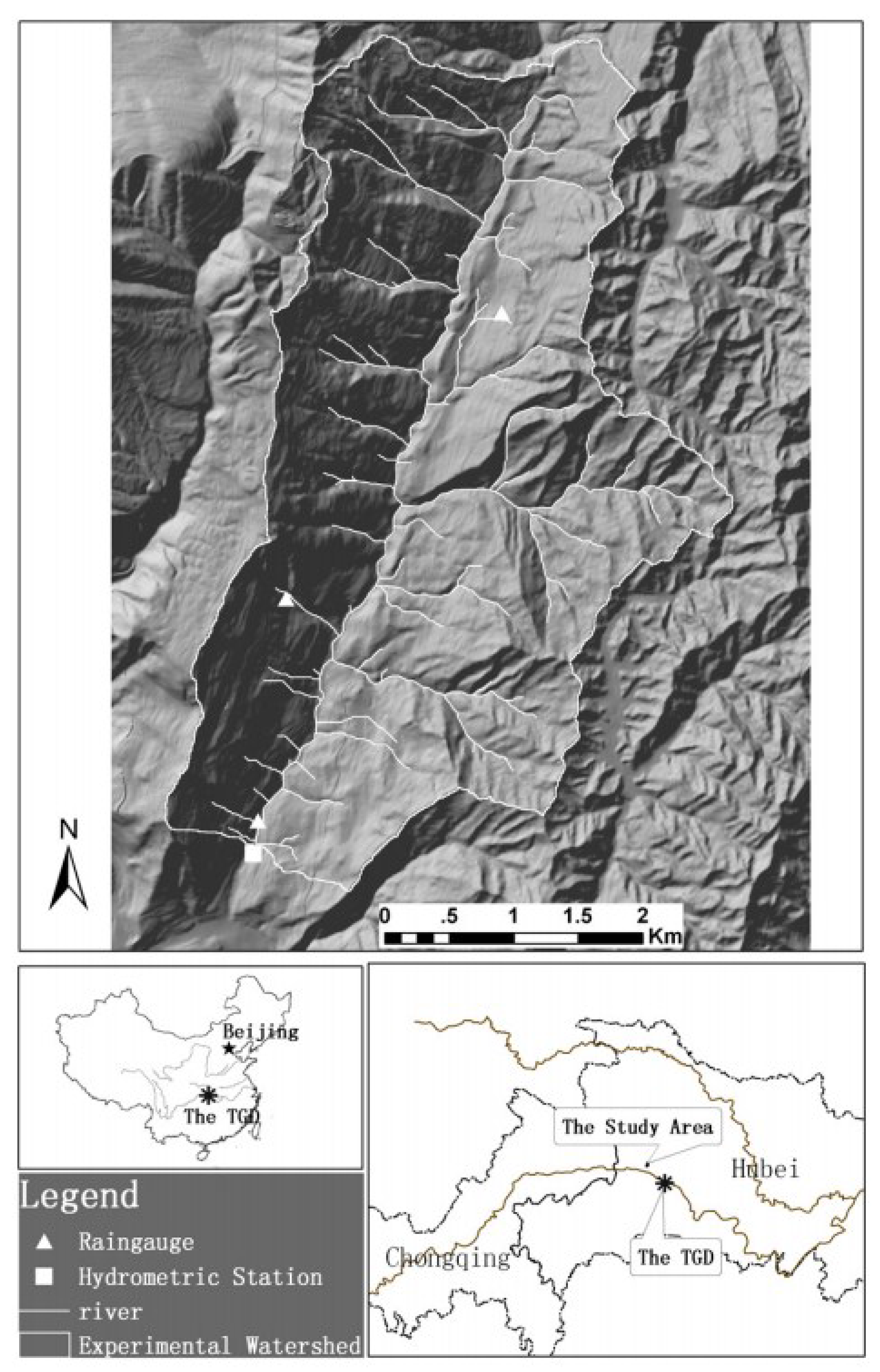
Figure 1 shows the study area of the Wangjiaqiao watershed which lies in Zigui County of Hubei Province, China. It is located at latitude 31°5′ N and 31°9′ N to longitude 110°40′ N and 110°43′ N. The total area of this study site is 1670 hectares and it is about 50 km northwest of the Three-Gorges Dam. Twenty nine rainfall–runoff data pairs were collected from 1994 to 1996 as shown in

Table 1. Rainfall-runoff data of Wangjiaqiao watershed [13].

No.	Storm	Rainfall	Direct Runoff	Initial Abstraction	Retention	Ratio
	Event	P (mm)	Q (mm)	${\mathit{I}}_{\mathit{a}}$ (mm)	S (mm)	${\mathit{I}}_{\mathit{a}}/\mathit{S}$
1	03/05/1994	11.2	0.36	4.6	114.1	0.040
2	14/06/1995	11.9	0.16	6.5	176.9	0.037
3	24/04/1994	14.2	0.23	8.6	130.7	0.066
4	12/05/1995	19.0	0.01	16.8	481.8	0.032
5	16/04/1995	19.8	0.47	9.9	200.0	0.050
6	10/09/1995	22.0	0.03	18.1	503.1	0.036
7	01/06/1995	23.6	0.29	14.8	258.7	0.057
8	17/10/1995	24.1	0.48	13.6	218.0	0.062
9	09/05/1994	26.5	0.65	13.1	262.8	0.050
10	19/05/1995	27.1	1.78	10.0	146.9	0.068
11	19/06/1996	28.3	2.18	13.4	86.9	0.154
12	20/06/1995	30.8	4.02	8.3	103.4	0.080
13	29/07/1996	31.7	0.92	10.7	458.3	0.023
14	23/06/1996	32.3	1.27	6.1	514.7	0.012
15	28/06/1996	32.4	1.75	14.6	163.3	0.089
16	14/05/1996	36.1	3.45	8.9	187.2	0.048
17	18/04/1994	38.1	3.72	10.4	178.6	0.058
18	19/10/1995	41.2	1.75	8.6	574.0	0.015
19	26/08/1994	48.1	1.08	19.0	755.2	0.025
20	04/06/1994	49.7	2.88	9.3	525.7	0.018
21	04/11/1996	49.8	4.15	6.7	405.1	0.017
22	07/07/1995	51.9	11.25	12.1	100.9	0.120
23	02/07/1996	54.0	2.86	7.4	714.0	0.010
24	02/05/1996	57.7	5.34	21.6	207.8	0.104
25	03/06/1996	62.1	3.23	18.5	544.6	0.034
26	07/06/1994	68.6	11.87	11.3	219.2	0.052
27	09/04/1994	73.7	9.94	14.1	297.6	0.047
28	18/09/1996	82.3	15.70	16.7	208.6	0.082
29	03/07/1996	85.9	21.31	7.8	208.1	0.037

[13].

3.2. Runoff Model Assessment

To measure the effectiveness of the proposed method, the Nash–Sutcliffe index (E), the model residual sum of square errors ($RSS$) and the overall model prediction error ($BIAS$) were computed using Equations (9)–(11) respectively.

$$\begin{array}{ccc}\hfill E& =& 1-{\displaystyle \frac{RSS}{{\sum }_{i=1}^n{(Q_{predicted}-Q_{mean})}^2}}\hfill \end{array}$$

(9)

$$\begin{array}{ccc}\hfill RSS& =& \sum _{i=1}^n{(Q_{predicted}-Q_{observed})}^2\hfill \end{array}$$

(10)

$$\begin{array}{ccc}\hfill BIAS& =& {\displaystyle \frac{{\sum }_{i=1}^n(Q_{predicted}-Q_{observerd})}{n}},\hfill \end{array}$$

(11)

where n is the total rainfall–runoff events of this study.

$RSS$ shows the model residual or prediction error. Thus, a predictive model with a lower $RSS$ value is able to predict runoff amount better. Meanwhile, $BIAS$ shows the overall model prediction error by the summation of a model residual (prediction error). A predictive model with zero $BIAS$ value is able to achieve perfect runoff prediction results, whereas positive $BIAS$ value indicates the model tendency to over predict runoff amount and vice versa. Lastly, E index value is used to determine the model prediction efficiency of a model. E index ranges from $-\infty$ to $1.0$, where $1.0$ implies a perfectly predictive model [32]. E index values between 0 and 1 are generally viewed as acceptable levels of performance; however, when $E<0$, the use of the mean runoff value observed can even predict the dataset better than the predictive model [33].

3.3. Results and Discussion

3.3.1. Inferential Statistics Assessment to Obtain Optimum $\lambda$ and S

In total, 29 different pairs of $\lambda$ and S values were derived from the rainfall–runoff data pairs of Wangjiaqiao watershed. At $\alpha =0.01$ level, the proposed method searched for the optimum value within the CI range of mean and median $\lambda$ values. Finally, an optimized pair of S and $\lambda$ values was used to represent the watershed. The descriptive statistics of $\lambda$ and S values were tabulated in

Table 2. Descriptive Statistical Results of $\lambda$ and S at Bias Corrected and Accelerated (BCa) 99% Confidence Interval.

Wangjiaqiao Datasets	Descriptive Statistics of $\mathit{\lambda }$	BCa 99% Confidence Interval		Descriptive Statistics of S	BCa 99% Confidence Interval
		Lower	Upper		Lower	Upper
Mean	0.053	0.069	0.384	308.477	230.413	395.527
Median	0.048	0.035	0.062	219.188	178.561	458.348
Skewness	1.251	0.268	1.846	0.867	−0.160	2.275
Kurtosis	1.884	−0.786	4.830	−0.389	−1.833	6.030
Std. Deviation	0.034	0.021	0.044	192.843	137.400	232.351

.

Other than referring to the skewness and kurtosis values for $\lambda$ and S dataset, the median value will be a better collective representation for $\lambda$ and S dataset to represent the watershed, as the Shapiro–Wilk normality test also concluded that $p<0.05$ for both $\lambda$ and S dataset. As the data distribution for both $\lambda$ and S dataset are not normally distributed by nature, the best collective $\lambda$ and S values were optimized within the median confidence interval ranges of $\lambda$ and S at $\alpha =0.01$ level to minimize the $RSS$ between the model predicted runoff amount and its observed values for the Wangjiaqiao dataset.

The optimum $\lambda$ value was 0.043 while 260.081 mm was the optimum S value (denoted as: $S_{0.043}$). The product of the optimum S and $\lambda$ value yield the initial abstraction ($I_a$) of 11.19 mm which was smaller than the smallest rainfall amount in the dataset from [13]. It fulfilled the $SCS$ constraints, whereby the $I_a$ amount must be met before any runoff process. Thus, based on the proposed watershed-specific $SCS$-$CN$ calibration method, the runoff depth (Q) for the Wangjiaqiao watershed in China can be computed using Equation (12).

$$Q_{0.043}={\displaystyle \frac{{(P-11.19)}^2}{P+248.891}}.$$

(12)

Based on Table 2, neither the mean nor the median BCa 99% $\lambda$ CI includes the value of 0.20, and therefore, a $\lambda$ value of 0.20 is not even statistically significant for the dataset of [13] at $\alpha =0.01$ level. Furthermore, the standard deviation for $\lambda$ at BCa 99% level is 0.034 with 77.14% $\lambda$ fluctuation percentage between its lower and upper CI ranges to show that $\lambda$ cannot be a constant but a variable due to its high fluctuation nature.

3.3.2. Watershed-Specific S Correlation Equation and $CN$ for Wangjiaqiao Watershed in China

In the study of [13], they referred to the S correlation equation mapped by [18] where the median $\lambda$ value of 0.05 was reported as the better collective representation for US watersheds. According to [18], a S correlation equation is required to convert the conjugate $CN$ value when $\lambda$ is no longer equal to 0.20. A different $\lambda$ value will lead to different corresponding S value and the $CN$ value will change accordingly. This study used Equation (8) to substitute $\lambda =0.043$ and 0.20 with respective rainfall–runoff data pairs to calculate the corresponding $S_{0.043}$ and $S_{0.20}$ values in order to determine the S correlation equation between $S_{0.043}$ and $S_{0.20}$ values for Wangjiaqiao watershed in SPSS. Equation (6) should not be adopted as it was derived (in inches) to reflect watershed conditions of the United States of America [18].

$SCS$ practitioner(s) will choose the $CN$ value from the NEH handbook and calculate the S value with Equation (4) which was proposed by $SCS$ under the hypothesis that $\lambda =0.20$. This study used the reverse methodology to convert the $S_{0.043}$ value into an equivalent $S_{0.20}$ value through a mapped watershed-specific S correlation equation in order to determine the watershed-specific $CN$ ($C{N}_{0.20}$). SPSS mapped the best S correlation equation between $S_{0.043}$ and $S_{0.20}$, as shown in Equation (13).

$$S_{0.2}={\left(S_{0.043}\right)}^{0.823}.$$

(13)

The correlation in Equation (13) has a lower standard error of 0.228 mm; the adjusted $R^2$ (Adj $R^2$) is equal to 0.998; and its p value is less than 0.001. As the optimum $S_{0.043}=260.081$ mm, the equivalent $S_{0.20}$ value can be found by using Equation (13) with 97.39 mm, leading to the calculated watershed-specific $CN$ value of 72.28 with Equation (4) for Wangjiaqiao watershed in China.

3.3.3. Asymptotic $CN$ of Wangjiaqiao Watershed

Many studies concluded that the $CN$ value could be derived with rainfall–runoff data pairs [34,35,36]. In 1993, the asymptotic $CN$ fitting method (AFM) was introduced to determine the $CN$ of a watershed with rainfall–runoff data pairs only [34]. At the WangJiaoQiao watershed, the standard $CN$ behavior was detected with AFM, whereas $CN$ stabilized at 65.10 (see Figure 2; hence, the equivalent $S_{0.2}$ value of the asymptotic $CN$ can be calculated with Equation (4) as 136.17 mm).

Furthermore, the $I_a$ value can be determined, as it is the multiplication of $\lambda$ and S values, and therefore, the $I_a$ value we got was 27.24 mm. However, ten out of twenty nine (34.48%) rainfall events observed in Table 1 are smaller than the calculated $I_a$ value. As such, AFM derived an $I_a$ value which was in conflict with the aforementioned $SCS$ constraint, one that meant there would be no runoff generated from any rainfall amount below the $I_a$ value.

3.3.4. Residual Modeling and the Corrected Equation

Some researchers developed new models or modified the existing $SCS$-$CN$ rainfall–runoff model by adding more parameters to improve surface runoff prediction accuracy [14,16,22,37,38,39,40,41,42,43,44]. However, those modified rainfall–runoff models could not solve the problem faced by $SCS$ practitioners or any software that has already integrated the conventional $SCS$-$CN$ model or embedded $\lambda =0.20$ into its software algorithm.

In order to correct the runoff prediction variance ($Q_v$) between the conventional $SCS$-$CN$ model and the new calibrated $SCS$-$CN$ model to benefit $SCS$ practitioners in their current practice, residual analyses of runoff predictive model were conducted between the two models to form a corrected equation, as shown in Equation (14). The $Q_v$ was mapped with several non-linear regression models in SPSS according to rainfall values.

$$Q_v=-0.00003P^3+0.007P^2-0.322P+3.511,$$

(14)

where $Q_v$ is the runoff prediction difference (mm) obtained by computing Equations (3)–(12) and P is the rainfall depth (mm).

Equation (14) shows the $Q_v$ between Equations (3) and (12). Positive $Q_v$ indicates that Equation (3) predicted a larger runoff amount compared to Equation (12). $Q_v$ can be plotted in order to visualize that Equation (3) produced inconsistent runoff prediction results, where it over predicted runoff when rainfall was less than 16 mm and more than 36 mm (see Figure 3) but under predicted the runoff amount when rainfall depth was between 16 mm and 36 mm. Equation (14) achieved an Adj $R^2$ near to 1.0 and low standard error of the estimate (0.053 mm) with statistical significance ($p<0.001$) to correct and improve the runoff prediction results of Equation (3). As such, Equation (14) can be amended to Equation (3) to improve the runoff prediction accuracy of Equation (3), as shown in Equation (15).

$$Q={\displaystyle \frac{{(P-0.2S)}^2}{P+0.8S}}-(-0.00003P^3+0.007P^2-0.322P+3.511),$$

(15)

where $P>0.2S$, else $Q=0$.

Equation (15) adjusted and improved the runoff prediction results of Equation (3). $RSS$ of Equation (3) was reduced by 66%; the over prediction tendency of the model was corrected by 96%; and achieved proximate runoff prediction results as the new calibrated $SCS$-$CN$ model, while the E index was improved by 71% to 0.826. Without model calibration, the conventional $SCS$-$CN$ model over-predicted runoff amount by almost 155,000 m³ at the rainfall depth of 85.90 mm when compared to the newly calibrated $SCS$-$CN$ model at the 1670 ha Wangjiaqiao watershed in China. The runoff over prediction risk would be even worse toward high rainfall intensities. On the other hand, it also under-predicted runoff amount up to 8000 m³ at the rainfall depth of 26.5 mm. This showed that the conventional $SCS$-$CN$ model was not only statistically insignificant at $\alpha =0.01$ level, but produced inconsistent runoff prediction results at different rainfall depths.

3.3.5. Comparison of Runoff Prediction Models

The law of parsimony favors a simple model with less fitting parameters. As such, this study explored the possibility of using a linear regressed rainfall–runoff model to quantify the runoff behavior at the Wangjiaqiao watershed. Past researchers proposed that the slope of a linear fitting equation could represent the total impervious area of a watershed while the fitting constant was regarded as the depression loss [45]. In this study, SPSS fitted the best linear regressed rainfall–runoff model for Wangjiaqiao watershed as: $Q=0.214P-4.623$ with an Adj $R^2$ = 0.715 and standard error of estimate was equal to 2.779 mm. Both fitting slope and constant parameter were statistically significant ($p<0.001$) but the model produced five out of twenty nine (17.2%) negative runoff prediction results.

$\lambda$’s confidence interval in Table 2 implies that $\lambda$ value cannot be 0.20 and a constant value at Wangjiaqiao watershed in China. As a result, the conventional $SCS$-$CN$ model becomes invalid and not statistically significant. When the $\lambda$ value is fixed at 0.20, the optimized $S_{0.20}=100.8$ mm and $I_a$ value can be calculated as 20.16 mm, but this $I_a$ value violated the $SCS$ constraint, as 17.24% of rainfall data pairs from [13] were less than the $I_a$ value. Thus, the conventional $SCS$-$CN$ model faced the same problem as the AFM and the linear regression model. Moreover, the conventional $SCS$-$CN$ model had the lowest E index; highest $RSS$; and $BIAS$ when compared to the AFM, the linear regression model and the newly calibrated watershed-specific $SCS$-$CN$ model. The statistics of five runoff predictive models were tabulated in

Table 3. Descriptive statistics of five runoff predictive models.

Model Parameters and Statistics	AFM Model	Calibrated SCS-CN Model Equation (12)	Conventional SCS-CN Model Equation (3)	Corrected SCS-CN Model Equation (15)	Linear Regression Model
p value	-	<0.001	Not Significant	Adjusted	<0.001
$\lambda$	0.200	0.043	0.200	0.200	-
S (mm)	136.19	260.08	100.80	-	-
$I_a$ (mm)	27.238	11.190	20.16	-	4.623
E	0.799	0.825	0.482	0.826	0.725
$RSS$	152.251	133.044	393.126	131.960	208.462
$BIAS$	−0.624	0.056	1.586	0.055	−0.008
$C{N}_{0.2}$	65.096	72.284	71.590	-	-
Residual Mean	−0.624	0.056	n/a	0.055	−0.008
BCa 99% CI
Range of	[−1.631, 0.283]	[−0.898, 0.961]	n/a	[−0.896, 0.970]	[−1.225, 1.124]
Mean Residual
Residual Median	n/a	n/a	0.140	n/a	n/a
BCa 99% CI
Range of	n/a	n/a	[−0.420, 3.850]	n/a	n/a
Median Residual
Standard
Deviation of	2.244	2.179	3.381	2.171	2.728
Model error
Variance (Residual)	5.035	4.748	11.429	4.715	7.445
Range	11.350	10.844	12.740	10.770	12.987
p value
of Shapiro-Wilk	0.197	0.111	0.012	0.121	0.597
Test

.

Residual analyses were conducted by using SPSS to measure the runoff prediction error of every runoff predictive model. The model with the smallest residual confidence interval range, lowest standard deviation error and variance was to be the best runoff predictive model of this study. The SPSS normality test showed that the significant value of the Shapiro–Wilk test was more than 0.05 for the AFM model, the newly calibrated watershed-specific $SCS$-$CN$ model, the corrected $SCS$-$CN$ model and the linear regression model; thus, their mean residual values were referred to for the accuracy comparison of the predictive model. On the other hand, the p value of the Shapiro–Wilk test for the conventional $SCS$-$CN$ model was less than 0.05; hence, its median residual values were used as the benchmark for its model accuracy.

The mean residual value of the newly calibrated, watershed-specific $SCS$-$CN$ model was among the lowest (0.056 mm) and nearest to zero, while its 99% BCa confidence interval range of mean residuals spanned across a small range when compared to other models. In addition, the newly calibrated, watershed-specific $SCS$-$CN$ model had a low residual variance and standard deviation which indicated that the newly calibrated runoff predictive model had the ability to achieve a runoff prediction with low error. As a result, the newly calibrated watershed-specific $SCS$-$CN$ model became a suitable runoff predictive model for the twenty nine data pairs at the Wangjiaqiao watershed in this study. On the other hand, the corrected $SCS$-$CN$ model also managed to correct runoff prediction errors of the conventional $SCS$-$CN$ model and achieved proximate runoff prediction results as the newly calibrated watershed-specific $SCS$-$CN$ model, which proves that the presented residual modeling technique was effective at transforming Equation (3) into a better rainfall–runoff model.

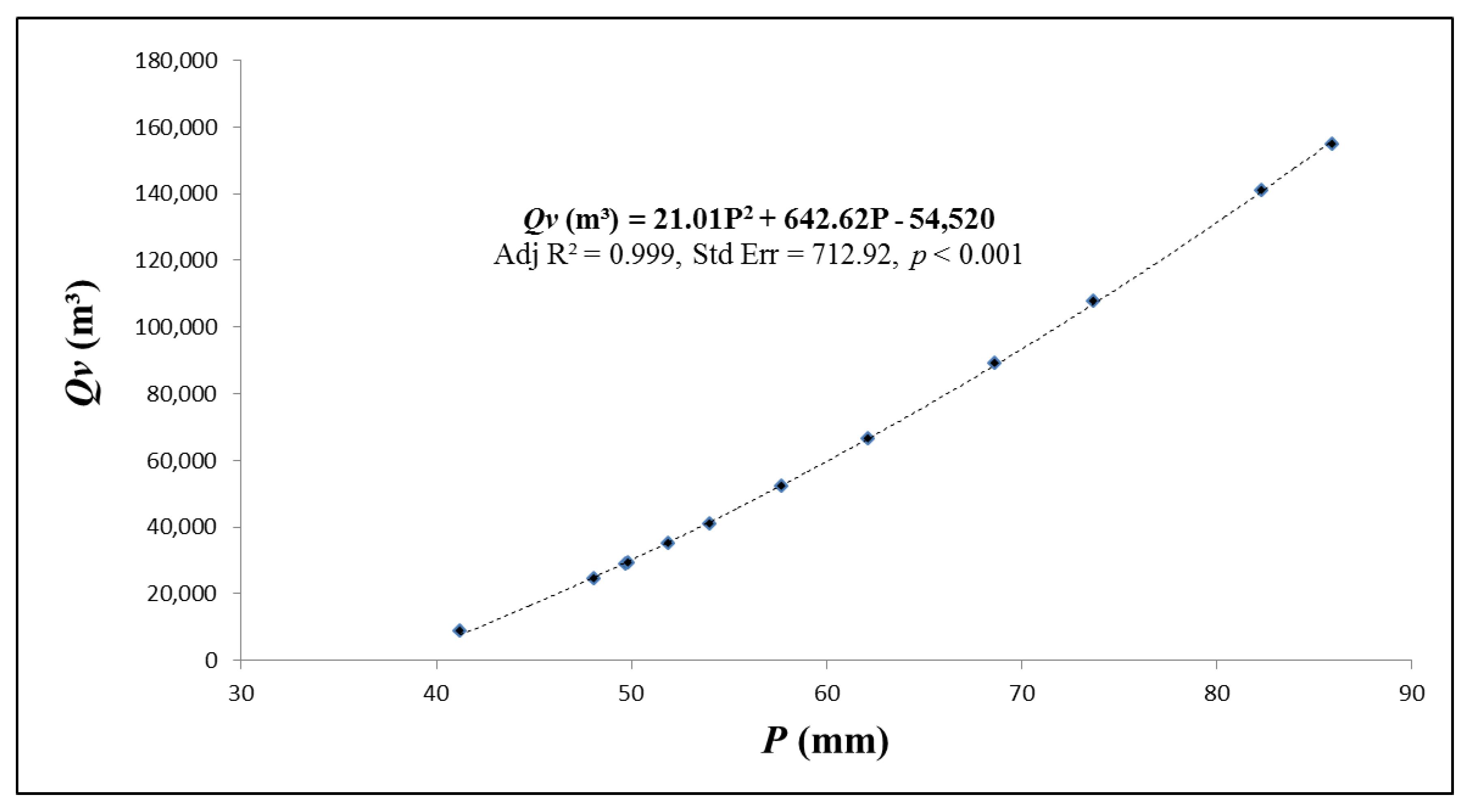
Without model calibration, the conventional $SCS$-$CN$ model over predicted runoff volume significantly from rainfall depths of 40 mm onward at the 1670 ha Wangjiaqiao watershed in China (see Figure 4). Through Equation (14), it is possible to quantify and model the runoff over prediction volume according to its corresponding rainfall depths. SPSS mapped that $Q_v$ (m³) $=21.01P^2+642.62P-\mathrm{54,520}$ was able to quantify the runoff over prediction volume from the conventional $SCS$-$CN$ model with and an Adj $R^2$ near to 1.0 and low standard error of 712.92 m³ ($p<0.001$).

4. Conclusions

A new watershed-specific $SCS$-$CN$ calibration method was proposed to identify the optimum $\lambda$ and S values, and derive $CN$ with the use of non-parametric inferential statistics, the rainfall-runoff data pairs and the supervised non-linear numerical optimization technique. The proposed model was applied to the Wangjiaqiao watershed in China. Inferential statistics showed that the conventional $SCS$-$CN$ model was not statistically significant at $\alpha =0.01$ level, and therefore, it was not applicable to model the runoff conditions of the Wangjiaqiao watershed in China. The proposed model identified the optimum median $\lambda$ of 0.043 (with the 99% confidence interval ranging from 0.035 to 0.062) as the best collective $\lambda$ for the Wangjiaqiao watershed. A watershed-specific S correlation equation was mapped in this study to show that the $CN$ value of the Wangjiaqiao watershed can be derived directly without referring to the NEH handbook. The estimated $CN$ of Wangjiaqiao watershed in China was 72.28 with a 99% confidence interval ranging from 62.06 to 78.0.

The newly calibrated watershed-specific $SCS$-$CN$ model improved the previous study results: the E index increased by 7.4%, the $BIAS$ of predictive model was reduced by 93.8% and model’s $RSS$ was lowered by 24.4%. These improvements were achieved with a $\lambda$ of 0.043 instead of rounding it to 0.050. The proposed model also outperformed the AFM model, the conventional $SCS$-$CN$ model and the linear regression model to predict runoff amount at the Wangjiaqiao watershed. The proposed model had the lowest $BIAS$ and $RSS$, and the highest E index when compared to those runoff predictive models. On the other hand, the linear regression model had the second highest model inaccuracy after the conventional $SCS$-$CN$ model, and both models produced negative runoff prediction results that were unable to yield a meaningful hydrological interpretation to predict surface runoff at the Wangjiaqiao watershed. Both models were also unable to produce positive runoff prediction results for rainfall depths less than 20 mm.

A runoff corrected equation was formulated through the proposed residual modeling technique under this study. The equation managed to correct runoff inconsistencies of the conventional $SCS$-$CN$ model and improved its runoff prediction accuracy. The S correlation equation from other study cannot be adopted as it reflects specific watershed conditions. It must be derived with watershed-specific $\lambda$ and rainfall–runoff data pairs in order to convert the $C{N}_{\lambda }$ into an equivalent $C{N}_{0.20}$. This study also found that the rounding of $\lambda$ and $CN$ values will induce the runoff prediction errors. As a result, $CN$ with at least two decimal places is recommended to $SCS$ practitioners for their future studies.

Based on the proposed SCS-CN calibration method, Equation (12) is recommended for the runoff prediction of the dataset from [13] at the Wangjiaqiao watershed in the Three Gorges Area. When a new rainfall–runoff dataset becomes available, SCS practitioners should re-derive the calibrated SCS runoff model again with the proposed methodology.

References

- Wang, Z.; Jiao, J.; Rayburg, S.; Wang, Q.; Su, Y. Soil erosion resistance of “Grain for Green” vegetation types under extreme rainfall conditions on the Loess Plateau, China. Catena 2016, 141, 109–116. [Google Scholar] [CrossRef]
- Zhou, J.; Fu, B.; Gao, G.; Lü, Y.; Liu, Y.; Lü, N.; Wang, S. Effects of precipitation and restoration vegetation on soil erosion in a semi-arid environment in the Loess Plateau, China. Catena 2016, 137, 1–11. [Google Scholar] [CrossRef]
- Chen, H.; Zhang, X.P.; Abla, M.; Lu, D.; Yan, R.; Ren, Q.F.; Ren, Z.Y.; Yang, Y.H.; Zhao, W.H.; Lin, P.F. Effects of vegetation and rainfall types on surface runoff and soil erosion on steep slopes on the Loess Plateau, China. Catena 2018, 170, 141–149. [Google Scholar] [CrossRef]
- Merritt, W.S.; Letcher, R.A.; Jakeman, A.J. A review of erosion and sediment transport models. Environ. Model. Softw. 2003, 18, 761–799. [Google Scholar] [CrossRef]
- Beven, K. Changing ideas in hydrology—The case of physically based models. J. Hydrol. 1989, 105, 157–172. [Google Scholar] [CrossRef]
- Ferro, V.; Minacapilli, M. Sediment delivery processes at basin scale. Hydrol. Sci. J. 1995, 40, 703–717. [Google Scholar] [CrossRef] [Green Version]
- Loague, K.; Freeze, R.A. Comparison of rainfall-runoff modeling techniques on small upland catchments. Water Resour. Res. 1985, 21, 229–248. [Google Scholar] [CrossRef]
- Perrin, C.; Michel, C.; Andreassian, V. Does a large number of parameters enhance model performance? Comparative assessment of common catchment model structures on 429 catchments. J. Hydrol. 2001, 242, 275–301. [Google Scholar] [CrossRef]
- Steefel, C.I.; Van Cappellan, P. Reactive transport modeling of natural systems. J. Hydrol. 1998, 209, 1–7. [Google Scholar]
- Kleissen, F.; Beck, M.; Wheater, H. The identifiability of conceptual hydrochemical models. Water Resour. Res. 1990, 26, 2979–2992. [Google Scholar] [CrossRef]
- SCS National Engineering Handbook (SCS NEH). Section 4, Hydrology, Chapter 21. In National Engineering Handbook; SCS: Washington, DC, USA, 1965. [Google Scholar]
- Shi, P.J.; Yuan, Y.; Zheng, J.; Wang, J.A.; Ge, Y.; Qiu, G.Y. The effect of land use/cover change on surface runoff in Shenzhen region, China. Catena 2007, 69, 31–35. [Google Scholar] [CrossRef]
- Shi, Z.H.; Chen, L.D.; Fang, N.F.; Qin, D.F.; Cai, C.F. Research on the SCS-CN initial abstraction ratio using rainfall- runoff event analysis in the Three Gorges Area, China. Catena 2009, 77, 1–7. [Google Scholar] [CrossRef]
- Jain, M.K.; Mishra, S.K.; Babu, S.; Singh, V.P. Enhanced runoff curve number model incorporating storm duration and a non-linear Ia-S relation. J. Hydrol. Eng. ASCE 2006, 11, 631–635. [Google Scholar] [CrossRef]
- Ponce, V.M.; Hawkins, R.H. Runoff curve number: Has it reached maturity? J. Hydrol. Eng. 1996, 1, 11–19. [Google Scholar] [CrossRef]
- Mishra, S.K.; Singh, V.P. Long-term hydrological simulation based on the soil conservation service curve number. Hydrol. Process 2004, 18, 1291–1313. [Google Scholar] [CrossRef]
- Baltas, E.A.; Dervos, N.A.; Mimikou, M.A. Technical note: Determination of the SCS initial abstraction ratio in an experimental watershed in Greece. Hydrol. Earth Syst. Sci. 2007, 11, 1825–1829. [Google Scholar] [CrossRef] [Green Version]
- Hawkins, R.H.; Ward, T.J.; Woodward, D.E.; Van Mullem, J.A. Curve Number Hydrology: State of Practice; American Society of Civil Engineers: Reston, VI, USA, 2009. [Google Scholar]
- Fu, S.; Zhang, G.; Wang, N.; Luo, L. Initial abstraction ratio in the SCS-CN method in the Loess Plateau of China. Trans. ASABE 2011, 54, 163–169. [Google Scholar] [CrossRef]
- D’Asaro, F.; Grillone, G. Empirical investigation of curve number method parameters in the Mediterranean area. J. Hydrol. Eng 2012, 17, 1141–1152. [Google Scholar] [CrossRef]
- D’Asaro, F.; Grillone, G.; Hawkins, R.H. Curve number: Empirical evaluation and comparison with curve number handbook tables in Sicily. J. Hydrol. Eng. 2014, 19. [Google Scholar] [CrossRef]
- Singh, P.K.; Mishra, S.K.; Berndtsson, R.; Jain, M.K.; Pandey, R.P. Development of a modified SMA based MSCS-CN model for runoff estimation. Water Resour. Manag. 2015, 29, 4111–4127. [Google Scholar] [CrossRef]
- Ross, C.; Prihodko, L.; Anchang, J.; Kumar, S.; Ji, W.; Hanan, N. HYSOGs250m, global gridded hydrologic soil groups for curve-number-based runoff modeling. Sci. Data 2018, 5, 1–8. [Google Scholar] [CrossRef] [PubMed]
- Jaafar, H.; Ahmad, F.; El Beyrouthy, N. GCN250, new global gridded curve numbers for hydrologic modeling and design. Sci. Data 2019, 6, 1–8. [Google Scholar] [CrossRef] [PubMed] [Green Version]
- National Engineering Handbook (NEH). Part 630 Hydrology. In National Engineering Handbook; USDA: Washington, DC, USA, 2004. [Google Scholar]
- Efron, B.; Tibshirani, R. An Introduction to the Bootstrap; Chapman & Hall/CRC: Boca Raton, FL, USA, 1994; ISBN 978-0-412-04231-7. [Google Scholar]
- Davison, A.C.; Hinkley, D.V. Bootstrap methods and their application. In Cambridge Series in Statistical and Probabilistic Mathematics; Cambridge University Press: Cambridge, UK, 1997; ISBN 0-521-57391-2. [Google Scholar]
- Efron, B. Large-Scale Inference: Empirical Bayes Methods for Estimation, Testing and Prediction; Institute of Mathematical Statistics Monographs, Cambridge University Press: Cambridge, UK, 2010; ISBN 978-0-521-19249-1. [Google Scholar]
- Rochoxicz, J.A., Jr. Bootstrapping Analysis, Inferential Statistics and EXCEL. Spreadsheets Educ. 2011, 4, 4. [Google Scholar]
- Schneider, L.E.; McCuen, R.H. Statistical guidelines for curve number generation. J. Irrig. Drain. Eng. 2005, 131, 282–290. [Google Scholar] [CrossRef]
- Andy, F. Discovering Statistics Using IBM SPSS, 4th ed.; SAGE Publications: Thousand Oaks, CA, USA, 2013; pp. 595–609. [Google Scholar]
- Nash, J.; Sutcliffe, J. River flow forecasting through conceptual models part 1 - A discussion of principles. J. Hydrol. 1970, 10, 282–290. [Google Scholar] [CrossRef]
- Moriasi, D.N.; Arnold, J.G.; Van Liew, M.W.; Bingner, R.L.; Harmel, R.D.; Veith, T.L. Model evaluation guidelines for systematic quantification of accuracy in watershed simulations. Trans. ASABE 2007, 50, 885–900. [Google Scholar] [CrossRef]
- Hawkins, R.H. Asymptotic determination of runoff curve numbers from data. J. Irrig. Drain. Eng. 1993, 119, 334–345. [Google Scholar] [CrossRef]
- Soulis, K.X.; Valiantzas, J.D.; Dercas, N.; Londra, P.A. Investigation of the direct runoff generation mechanism for the analysis of the SCS-CN method applicability to a partial area experimental watershed. Hydrol. Earth Syst. Sci. 2009, 13, 605–615. [Google Scholar] [CrossRef] [Green Version]
- Soulis, K.X.; Valiantzas, J.D. Identification of the SCS-CN parameter spatial distribution using rainfall-runoff data in heterogeneous watersheds. Water Resour. Manag. 2013, 27, 1737–1749. [Google Scholar] [CrossRef]
- Mishra, S.K.; Singh, V.P. SCS-CN method. Part-I: Derivation of SCS-CN based models. Acta Geophy. Pol. 2002, 50, 457–477. [Google Scholar]
- Mishra, S.K.; Singh, V.P. Soil Conservation Service Curve Number (SCS-CN) Methodology; Kluwer: Dordrecht, The Netherlands, 2003; ISBN 1-4020-1132-6. [Google Scholar]
- Sahu, R.K.; Mishra, S.K.; Eldho, T.I.; Jain, M.K. An advanced soil moisture accounting procedure for SCS curve number method. Hydrol. Process. 2007, 21, 2872–2881. [Google Scholar] [CrossRef]
- Kim, N.W.; Lee, J. Temporally weighted average curve number method for daily runoff simulation. Hydrol. Process. 2008, 22, 4936–4948. [Google Scholar] [CrossRef]
- Wang, S.; Kang, S.; Zhang, L.; Li, F. Simulation of an agricultural watershed using an improved curve number method in SWAT. Trans. ASABE 2008, 51, 1323–1339. [Google Scholar] [CrossRef]
- Ajmal, M.; Moon, G.; Ahn, J.; Kim, T. Investigation of SCS-CN and its inspired modified models for runoff estimation in South Korean watersheds. J. Hydro-Environ. Res. 2015, 9, 592–603. [Google Scholar] [CrossRef]
- Ajmal, M.; Waseem, M.; Wi, S.; Kim, T. Evolution of a parsimonious rainfall–runoff model using soil moisture proxies. J. Hydrol. 2015, 530, 623–633. [Google Scholar] [CrossRef]
- Ajmal, M.; Khan, T.A.; Kim, T.W. A CN-based ensembled hydrological model for enhanced watershed runoff prediction. Water 2016, 8, 20. [Google Scholar] [CrossRef] [Green Version]
- Arnbjerg-Nielsen, K.; Harremoes, P. Prediction of hydrological reduction factor and initial loss in urban surface runoff from small ungauged catchments. Atmos. Res. 1996, 42, 137–147. [Google Scholar] [CrossRef]
Figure 1.
Location of study area in Wangjiaqiao watershed, China [13].
Figure 2.
Standard behavior pattern, for Wangjiaqiao watershed.
Figure 3.
Runoff difference between the proposed calibrated model and the conventional - model.
Figure 4.
Runoff volumetric differences between the proposed, calibrated - model and the conventional - model.