Leak Localization in Water Distribution Networks Using Pressure and Data-Driven Classifier Approach

1
Advanced Control Systems Group at the Institut de Robòtica i Informàtica Industrial (CSIC-UPC), Llorens i Artigas, 4–6, 08028 Barcelona, Spain
2
CETaqua, Water Technology Centre, 08904 Barcelona, Spain
*
Author to whom correspondence should be addressed.
Water 2020, 12(1), 54; https://doi.org/10.3390/w12010054
Submission received: 15 November 2019
/
Revised: 2 December 2019
/
Accepted: 19 December 2019
/
Published: 21 December 2019
(This article belongs to the Section Water Resources Management, Policy and Governance)
Abstract
:Leaks in water distribution networks (WDNs) are one of the main reasons for water loss during fluid transportation. Considering the worldwide problem of water scarcity, added to the challenges that a growing population brings, minimizing water losses through leak detection and localization, timely and efficiently using advanced techniques is an urgent humanitarian need. There are numerous methods being used to localize water leaks in WDNs through constructing hydraulic models or analyzing flow/pressure deviations between the observed data and the estimated values. However, from the application perspective, it is very practical to implement an approach which does not rely too much on measurements and complex models with reasonable computation demand. Under this context, this paper presents a novel method for leak localization which uses a data-driven approach based on limit pressure measurements in WDNs with two stages included: (1) Two different machine learning classifiers based on linear discriminant analysis (LDA) and neural networks (NNET) are developed to determine the probabilities of each node having a leak inside a WDN; (2) Bayesian temporal reasoning is applied afterwards to rescale the probabilities of each possible leak location at each time step after a leak is detected, with the aim of improving the localization accuracy. As an initial illustration, the hypothetical benchmark Hanoi district metered area (DMA) is used as the case study to test the performance of the proposed approach. Using the fitting accuracy and average topological distance (ATD) as performance indicators, the preliminary results reaches more than 80% accuracy in the best cases.
1. Introduction
Water scarcity, leak detection, and network efficiency are the main factors driving the implementation of smart water solutions across the globe. Particularly, water leaks inside water distribution networks (WDN) can cause water losses in fluid transportation, risks of bacteria, and pollutant contamination [1]. Besides that, water leaks may also lead to increases in the consumers’ water bills, although in some countries (e.g., European and Canadian countries), higher water prices are connected with higher investment in the WDN in order to prevent leaks [2,3,4].
According to the standard water balance methodology presented by IWA/AWWA (International Water Association/American Water Works Association), water leakage is an important reason of water loss [5], as in many WDNs, the losses due to leaks are estimated to account for up to 27% of the total amount of extracted water [6]. In China, around 8 billion cubic meters of water was lost in 2017 [7], and the total amount in Asia is around 29 billion cubic meters (value more than 9 billion dollars) per year [8]. The mean value for water losses in EurEau (European Federation of National Associations of Water Services) member countries in the year of 2017 are 23% and 2171 m3/km/year [9]. Considering the worldwide problem of water scarcity, added to the challenges that a growing population brings, it is critical to minimize the water losses through the detection and localization of water leaks in the WDN in a timely and efficient manner using advanced techniques.
In order to accurately localize the water leaks, correct and oriented monitoring of detail information concerning system behavior is required. Among these monitoring devices, the acoustic equipment (e.g., noise correlators and listening sticks) is efficient to localize the leaks manually through reading abnormal behaviors at potential locations of the WDN system [10,11]. However, the expensive cost, as well as time consuming and labour demanding features prevent the acoustic equipment being widely used in reality. Due to that, flow and pressure meters are optional devices of reading useful system information for leak detection and localization. Compared with flow meters, pressure meters are easily installed and less expensive. Moreover, as discussed in [12], focusing more on using pressure data can facilitate leak localizations and reduce the required investments as well. The key principle of using real-time pressure measurements for leak detection and localization in WDNs is the deviation of real-time data from the normal range of system behaviors [11].
The state-of-the-art for leak localization in WDN is filled with contributions of different approaches. Among them, the original popular approaches rely on estimating hydraulic dynamics using mathematical models [13,14]. For example, [15] estimates the location of a leak through building a pressure drop surface with triangle-based cubic interpolation approach. Meanwhile, [16] infers a leak location in WDN through creating a sensitive matrix of different pressure measurements when a leak happens. However, the performance of model-based approaches is limited too much by the accuracy of the mathematical models, and it is not easy to choose an appropriate model [17]. Further, the investment requirement for a large number of sensors also slows down the development of this method. Moreover, the high computation demand and the difficulty of parameter estimations hinder the final usage of model-based approaches, especially for the large WDNs. During the past decades, with the advances of online monitoring devices, data-driven approaches which focus on the knowledge mining of available data have prevailed in the field of leak localization [11,12,18,19,20]. Accordingly, [18] proposes a mixed hydraulic and data-based model that relies on pressure residual and leak sensitivity analysis, which is based on analyzing the difference between measurements and their estimation using a hydraulic network model. More recently, [19] presented a completely data-driven approach through analyzing the pressure residual between a healthy WDN and a network with leakages, using [20] to interpolate the pressure in nodes without sensor information. However, due to the graph structure of the WDN, the accuracy of this approach is affected by the distance between the leaking and inlet node.
Due to the powerful capacities for pattern recognition and feature identification, a machine learning algorithm has been proven efficient for solving leak localization problems, using support vector machines and clustering algorithms, etc. [11,12]. However, the difficulty of using a machine learning method is selecting the proper algorithm and designing suitable feature extractors to learn complex features [11,12]. Among numerous machine learning approaches, the neural network (NNET) is a method which is capable of leak localization considering the ability of processing and modelling multiple inputs without explicit knowledge of the involved parameters. Further, linear discriminant analysis (LDA) is another method used in statistics and machine learning which explicitly attempts to find a linear combination of features to separate classes of objects. The high resolution of LDA makes this method a good tool to predict locations (e.g., leaks) based on limited information [21,22,23].
This work proposed a data-driven approach based on limit pressure measurements to localize a leak inside a WDN. Two different machine learning classifiers based on LDA and NNET are used to determine the probabilities of each node having a leak inside a WDN. In order to improve the localization accuracy, a Bayesian temporal reasoning is applied afterwards to rescale the probabilities of each possible leak location at each time step after a leak is detected. With the aim of achieving an accurate estimation of consumed water, the WDN has been divided into smaller sub-networks, named district metered areas (DMAs) for management. Almost all of the previous implementations are applied on the DMA level [10]. Practically, the performance of the leak localization methods is highly sensitive to the numbers of the installed sensors, as well as the placement of these sensors. In order to ensure the optimal performance of the proposed leak localization approaches, in this paper, the sensor placement strategies for a WDN from [24] are used directly without digging into this topic [24,25,26,27]. To estimate the nodes head where sensors are not placed, the Kriging spatial interpolation [20] with hydraulic topology of the network is used, which also generates a perfect no-leak scenario as a reference. Further, historical data for each leak scenario of each node are provided through simulation as training data for the classification. As an initial illustration, the benchmark Hanoi DMA is used as the case study to test performance of the proposed approach. Discussions about the costs and benefits of the proposed approach are also presented, as well as the future research plan.
2. Materials and Methods
2.1. Methodology
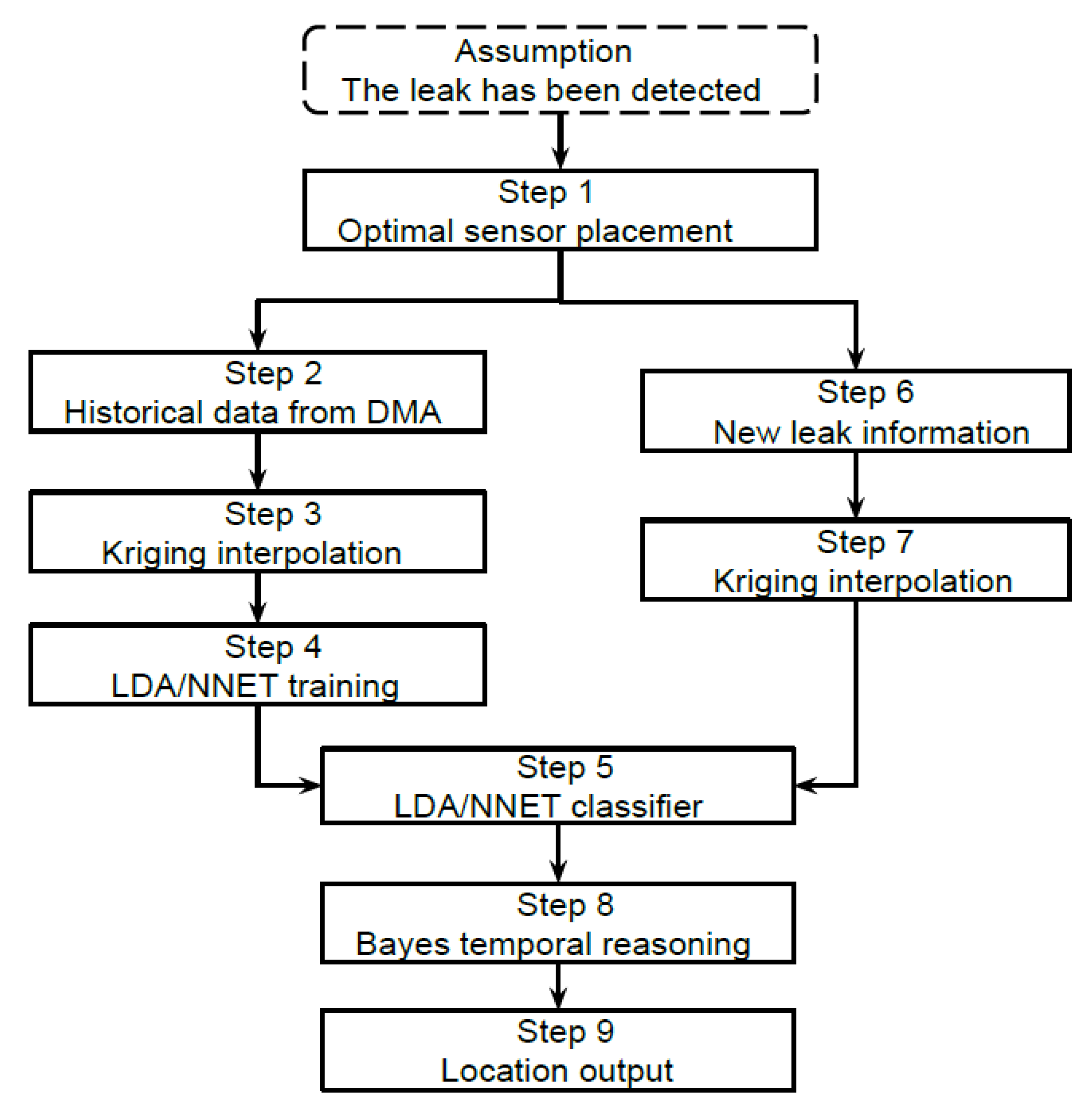
The scheme of the proposed pressure based data-driven leak localization approach [28] is depicted in Figure 1.
A key assumption has been made initially that a leak has already been detected in a DMA. Further, a number of pressure sensors is supposed to be installed to read pressure measurements for some nodes. A flow sensor is also required to read the inlet flow value to the DMA.
The first step of the proposed approach is selecting of the nodes with pressure sensor installed based on the optimal sensor placement strategy generated by [24]. Afterwards, datasets are prepared which include historical data of DMA comprising pressure measurements with corresponding leak location labels and flows at the inlet node. Topology information of the DMA is also needed to correctly interpolate for the nodes without sensors. More detailed definitions about the required datasets will be explained in the next section. After that, Kriging spatial interpolation is used in Step 3 to estimate the pressure at the nodes which are not equipped with sensors based on hydraulic proximity [29]. Later on, the machine learning classifiers in view of LDA and NNET are developed and trained using the datasets created at Step 2. The fitting accuracy, Kappa coefficient [30], and the average topological distance (ATD) are used as performance indicators for training the classifiers, and the best classifiers are selected to be used later on in Step 5. When a leak has been detected in Step 6, equal prior probabilities are initially set to all the nodes. Based on the limit pressure measurements from the sensors embedded in this DMA, as well as the estimated pressure interpolated by Kriging, the trained LDA/NNET classifiers are used to compute, in Step 5, probabilities of each node being the leak location based on raw pressure without estimating a hydraulic model nor a reference model. In order to better infer the leak node, the Bayes temporal reasoning rule is used at Step 8 to re-calibrate the probabilities given by the classifiers. The final estimated location of the leak is obtained at Step 9.
2.2. Data Structure
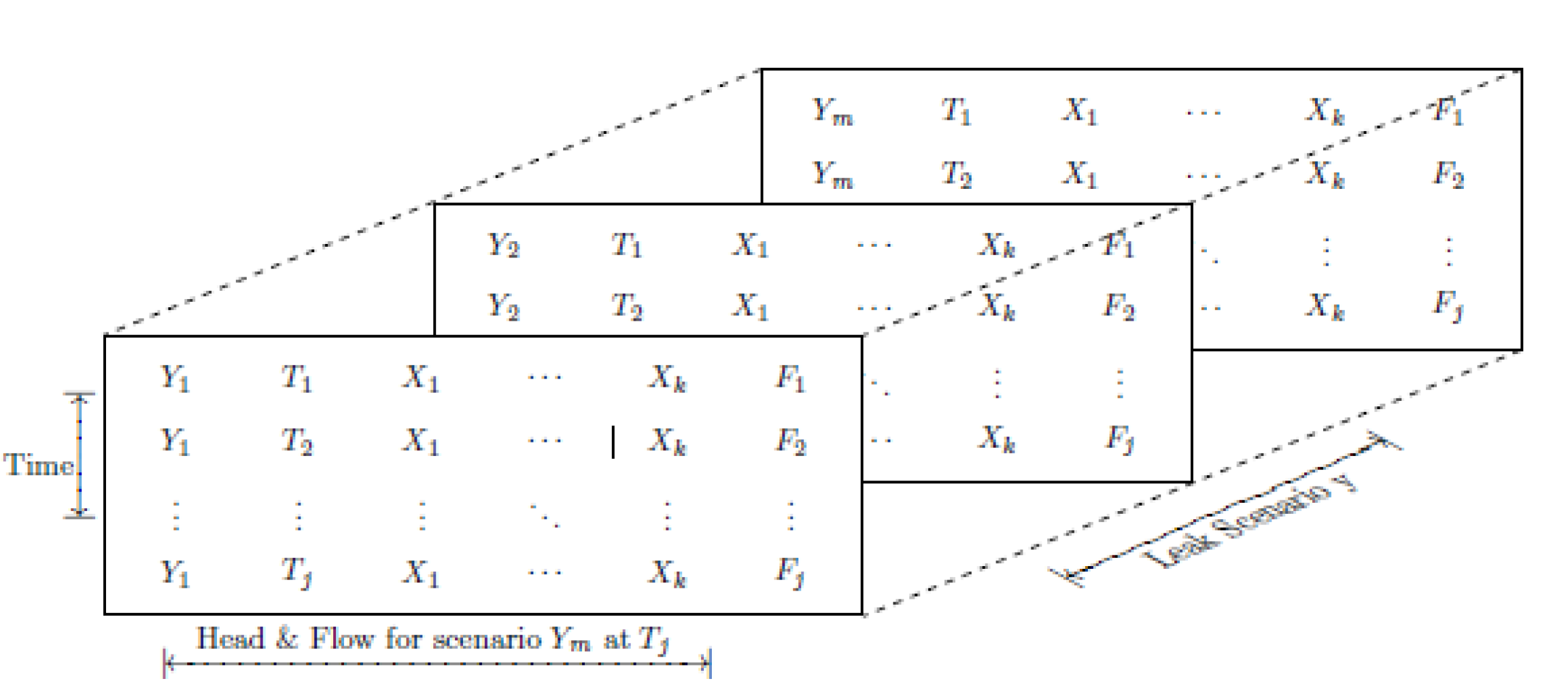
The data structure required for the leak localization approach is defined in a matrix (Figure 2) which contains: (1) The leak vector Y , which is a label where the true leak was located, and this information is assumed to be provided; (2) The time vector T in the unit of hour. The data structure is ordered by time, which is the time elapsed from when the leak was first created. As a leak has been detected, this information is also known; (3) The pressure vector X (m), which can actually either represents the head, pressure, or the residual with the reference model. The pressure information should be the value given directly from the sensors; (4) The flow vector F in the unit of m3/s. Flow from the inlet in the DMA, which is also the flow enters to the DMA, is the value provided by flow sensor measurement for analyzing.
The matrix should be read taking snapshots of the DMA at any given moment. So, for the leak scenario Y1, there is pressure Xk for the node k at given time Tj. The data set can be melted into a single matrix with each Y label repeated, which will be easier manipulated by RStudio, an open source software for R [31]. Considering there is not always a sensor at all the nodes, the pressures for the nodes which do not have a sensor is interpolated used Kriging, as explained in [19].
Table 1 includes an example of how the dataset should look:
2.3. Classifier
The classifiers in view of LDA and NNET are defined and tested individually with the objective of looking for a pattern where different leaks can be segregated to predict future events according to past historical data.
As explained in the introduction section, LDA [21] is a method to find a linear combination of features which separates two or more classes of data. The resulting combination may be used as a linear classifier. In this study, since there are more than two classes, multiclass LDA are used, in which a subspace is found in order to contain all the class variability. LDA models the distribution of the predictors (given X, in this study represents the node pressures) separately in each of the response classes (given Y, in this study means the different leak localization labels) and uses the Bayes theorem [32] to flip them into estimates. When these distributions are assumed to be normal, it turns out that the model is very similar to the logistic regression. Given the high complexity of calculation, the logistic regression in favor of LDA is omitted, which will be more efficient and deliver better results [33].
The NNET [34] fits a single-hidden-layer neural network trained for classification. Using cross-validation, the model has been tuned to both avoid over-fitting and setting the number of units in the hidden layer [33]. To avoid the over-fitting in the NNET, weight decay is used to penalize the sum of squares of the weights.
2.3.1. Cross Validation
In order to reduce over-fitting in the training set, 10-fold cross-validation is applied, which will consequently slow down the parameter process search. However, considering that the over-fitting is hard to removed entirely, a validation set is held out for the final estimation with expected prediction error. The cross-validation methods are defined as:
- Hold Out Method: Divide the training sample (70%) vs. testing sample (30%). If the error rate is similar on both, it means that the model is not over fitted. This method requires low computing time, however, it is prone to sample bias.
- K-Fold Cross Validation: The sample is spliced into K equal sub size samples. All of the models used have been calculated through a 10-fold cross validation. Since the response feature is categorical, the parameters will be tuned according to the results of accuracy. The K results can then be averaged to produce a single estimation. The upside of this method is that how to divide the data is less impactful, as selection bias will no longer be present.
2.3.2. Evaluation Metrics
The fitting accuracy, Kappa and ATD are the metrics being used to evaluate the classification performance in the dataset:
- Accuracy is the percentage of correctly classified instances out of all the instances. It is a more meaningful metric in binary classification than multi-class classification problems, since in multi-class problems it is harder to determine how the accuracy breaks down across the different classes.
- Kappa (or Cohen’s Kappa) is similar to classification accuracy, except that it is normalized at the baseline of random chance of the data [30]. It is a more useful measure to use on problems that have an imbalance in the classes. However, with the usage of simulations, this problem is negated, as all leak scenarios appear the same amount of times. It compares how the classifier performs against the performance of a classifier which simply guesses at random according to the frequency of each class. Values between 0.6 and 0.8 are considered good [35] even though they supplied no evidence to support it.
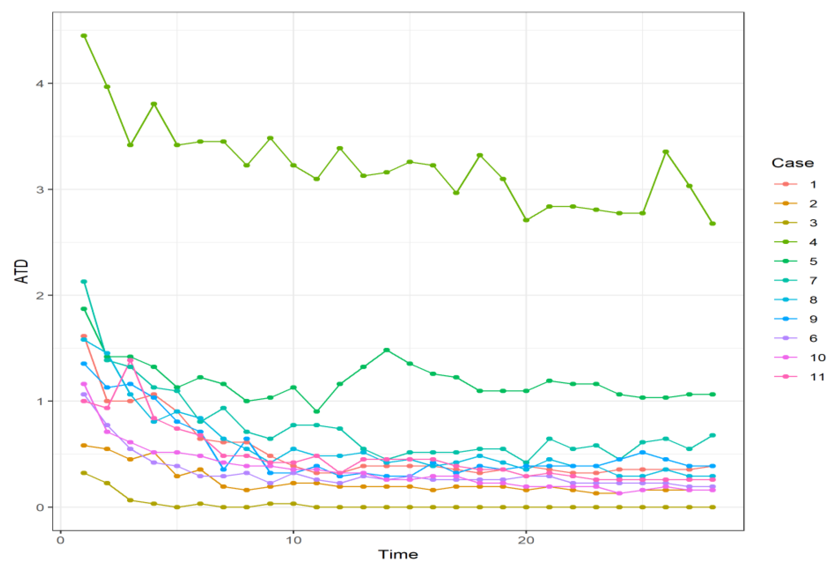
- ATD, average topological distance, which represents the distance in nodes between the node predicted as having the leak with the true node that has the leak. ATD is useful for node relaxation which will assess the overall performance.
Other than that, in the training phase of the model, fitting accuracy is also used as the metric for parameter tuning and for selecting the best model.
2.4. Bayes Temporal Reasoning
Bayes temporal reasoning has already been previously used to improve the diagnosis using the residuals generated in the model-based leak localization methodologies [19]. In this study, Bayesian temporal reasoning is used to improve the diagnosis in the proposed data-driven leak localization approach, working with probabilities given directly by the classifier which uses the head/pressure directly.
Due to the fact that the simulations of the dataset includes cases where a leak is created for a long period of time and the section with a healthy state in between the leaks is ignored, real situations cannot be fully represented. Besides that, in the healthy state, the leak localization procedure is irrelevant since the precondition is that a leak has been detected. All the leaks are also static, meaning, once created, it will present in the network until it is fixed.
Following this reasoning, a Bayes rule is added to re-scale the probabilities using as prior of the probabilities for each node being the candidate leak location at previous time steps. At every time step t, the probability of a leak occurrence is estimated as a result of the application of the Bayes rule:
where nl is the number of different leak labels, c(x(t)) is the probabilities returned by the classifier, LDA or NNET, given the head or pressure at time step t. P(yi|c(x(t))) is the posterior probability that the instance c(x(t)) belongs to the class yi at time step t given the previous information. P(c(x(t))|yi) is the likelihood of the instance c(x(t)) assuming that the leak has been created in node yi. P(yi|c(x(t − 1))) is the prior probability for the class yi taking into account previous time steps. P(c(x(t))) is a normalizing factor given by the total probability law:
At each iteration, the prior probabilities used are considered as equal for all different labels. The variable t = 1, …, k is the time step when a leak is first created until it is fixed, then P(yi|c(x(0))) = for i = 1, …, nl.
3. Case Study
3.1. Hanoi DMA
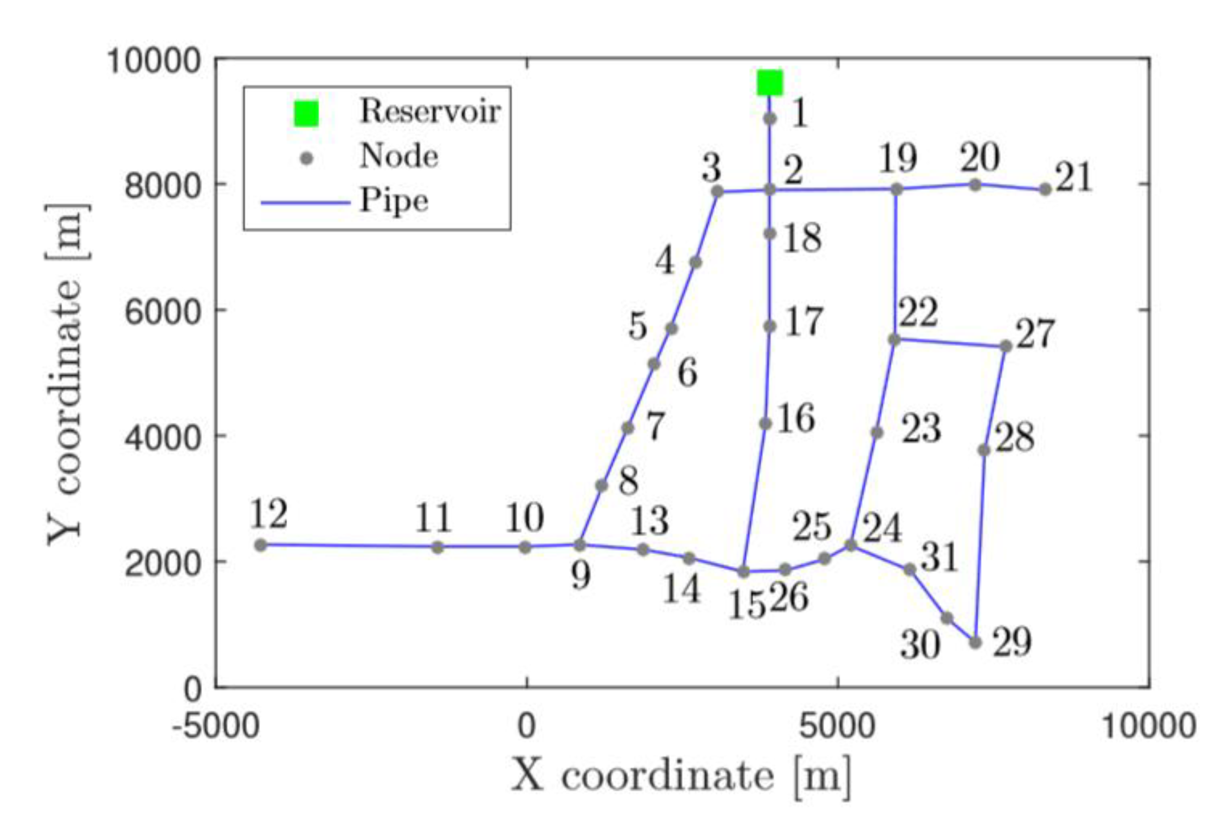
The Hanoi DMA (Figure 3) is used as the case study to initially illustrate the performance of the proposed approach. In this network, the reservoir acts as the inlet node of this DMA. Considering data for all the nodes are expected to generate, all the nodes are assumed have a sensor and the real distribution of the real sensor nodes placed inside the Hanoi network is ignored during the simulation phase. The simulation is obtained using the simulator EPANET 2 [36], where for each leak scenario, of the 31 nodes, a leak is simulated with one-hour time steps lasting 96 h. All the generated data from the simulation are used for calibrating the classifier models. A perfect case without leaks has been used as a reference.
3.2. Sensitivity Analysis with Residual
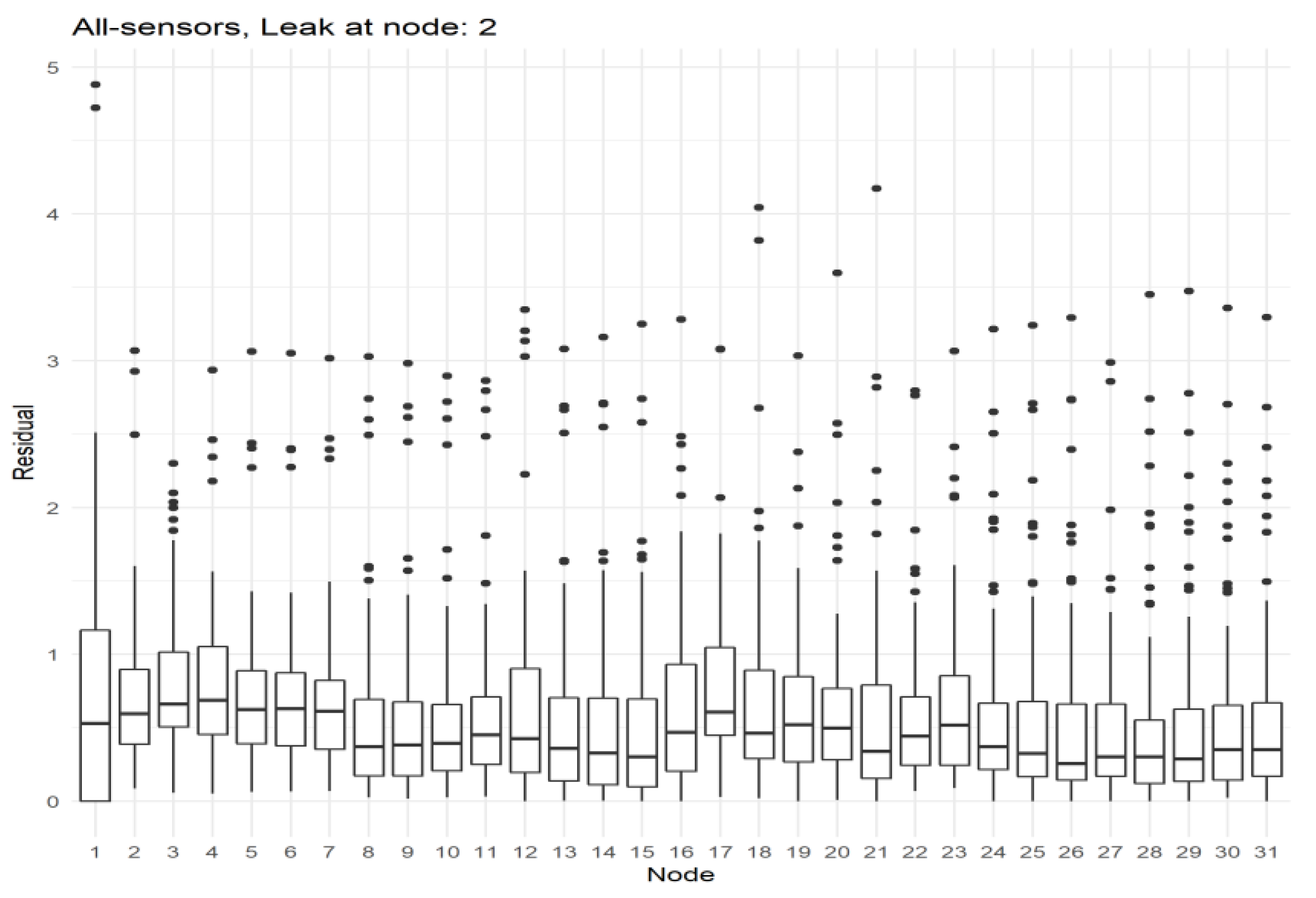
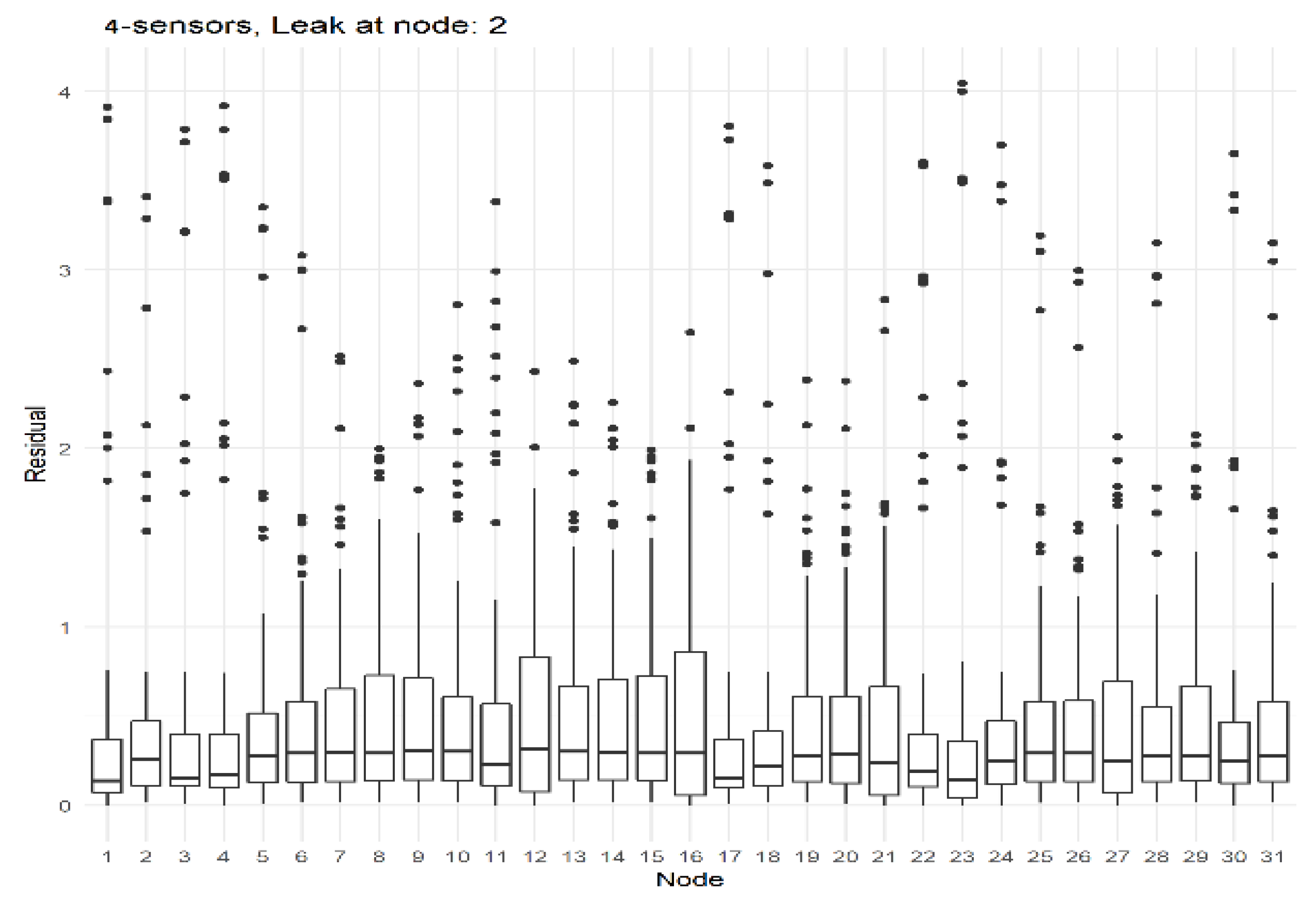
The state-of-the-art up has been that the node which has the highest difference (residual) between the reference model and the real time model should be the candidate which contains the leak. However, this is not always the case, especially when there are no sensors placed in all the different nodes inside the DMA. The following boxplots (Figure 4 and Figure 5) provide the distribution of residuals at each simulation time for all of the 31 leak scenarios, which shows that, the median for the node which contains the leak is, in most cases, is higher than the other groups. A significant increase is also observed with respect to the same node without a leak. However, other nodes which are topologically close to the true leak location have a higher median as well. Even when the leak is far away, it seems to obtain an increased residual compared to when there is not a leak in the network, affected by the topology of the DMA. Since these networks are graph structures by definition, once there is a leak in the DMA, the whole network is affected, and the network is limited in the choices to mitigate the leak. A node “previous” to the leak, in height or structure, will also be affected since the difference in head between its links will change, and the flow of water will modify its path accordingly. Nodes that are “posterior” to the leak, will also change from their default state, since the leak has been created. Water flows and pressure entering the posterior nodes will vary.
This hypothesis is further tested by checking the fringe nodes. On average, with the simulations, using the maximum residual approach accounted for a success rate of 28.5%. Of this 28.5%, 20% came from leaf nodes (in this case node 12 with an accuracy of 96.9% and node 21 with an accuracy of 86.5%). These nodes ranked the highest in success rate thanks to the fact that they are at the end of the network. Since they do not have “children” nodes, the error will not propagate along those links. However, 0% accuracy starting with node 10 and 11 also happen.
In these boxplots, it is clear to conclude that, leak localization is very dependent on the amount of nodes with sensors. A good result can be expected with sensors at all the nodes with respect to how the residual is much higher in the node which has the leak.
Finally, this approach is still reliant on Kriging to interpolate the pressure in nodes which do not have sensors placed. However, by the very definition of the problem, the assumption in which the variance of the field is stationary is at risk [37]. The creation of a leak inside the model will create an irregular event in which it is difficult to justify a stationary variance. The unknown evolution of the leak, and how irregular the variance will become once added to the model. With respect to the mean absolute percentage error, average errors are higher than 50%, except in the optimal four sensor placement, which is almost zero. Besides, after Kriging the amount of observations which surpassed three standard deviations was around 35% which indicates that the Kriging might not be working as well as we intended in this data.
3.3. Sensitivity Analysis with Pressures
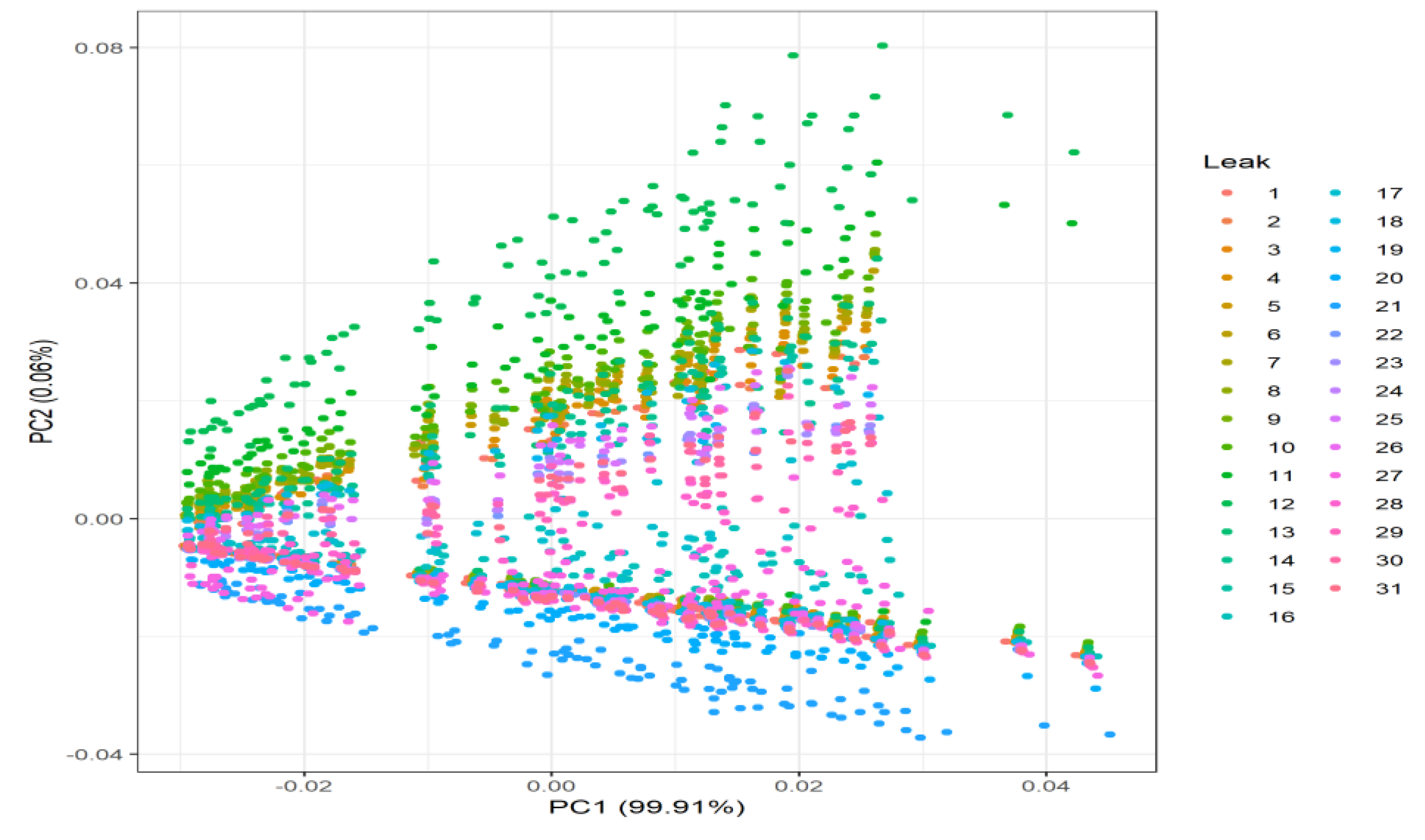
After the previous sensitivity analysis with residual, it is doubtful that the residuals are that useful at predicting the true leak location. A simpler approach using directly the pressure instead of the residual is taken. As explained in the methodology, only interpolate using Kriging once to obtain the head/pressure for all the nodes on the online model, omitting the reference model and residual calculations is considered.
Principal Component Analysis (PCA) [38] has been performed on the case with sensors at every node (Figure 6), and the non-perfect-information case (Figure 7), in which there are only four sensors placed inside the network (12, 16, 21, and 27) [24]. Removing time and flow features to see the structure of the data, a sort of rainbow effect can be detected, whereby thanks to the linear combination of pressures, it is able to differentiate where the different leak locations are. This, in turn, should translate to better and easier classification results when add to the flow.
3.4. Results
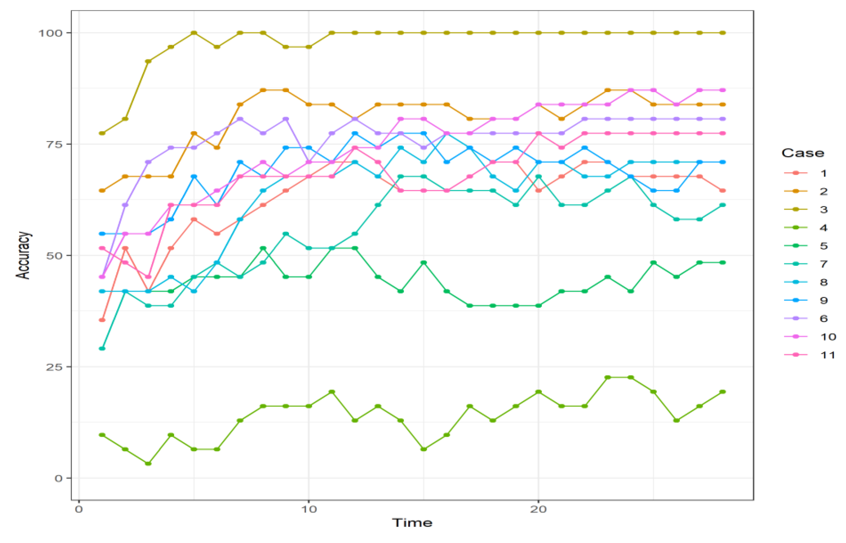
Following the method explained above, two different classifiers based on LDA and NNET are applied using R. The 72-h simulation from each leak scenario is used to train the model, and the 10-fold cross-validation is used to tune the parameters and to select the model with the best accuracy. Once trained, the resulting classifier is validated using the remaining 24 h to get accurate results of the evaluation metrics. Bayes time reasoning is also recursively applied on this validation data set.
Results in Table 2, Table 3 and Table 4 show how the NNET, when applied with posterior Bayes time reasoning, can result in around 70% accuracy in the average case. However, when there are five sensors placed in the network, very bad results are produced in both LDA and NNET. This might be due to the Kriging, in which the average error in this case was the worst compared to all the other sensor placement. This is not a new result, as it is known from posterior works that the placement of the sensors will produce very different results [39].
4. Conclusions
A new data-driven solution to the leak localization problem in WDNs based on limit pressure measurements has been presented in this study. The proposed approach has been explained or referred to, and an example is presented using the Hanoi DMA as case study.
After reviewing the results, the use of a reference model to calculate the residual is put into question. The main reason for this is that it hinders the data structure of the residuals by adding bias thanks to a not adequate Kriging estimation. As stated before, in the average case, the mean absolute percentage error is higher than 50% when applied to the interpolation. This fault is attributed to the Kriging assumptions, which do not hold in the network structure inherent to WDNs, as well as the intrinsic variability which a leak brings to the network.
As is common in the field, the number of sensors, and moreover the placement of these sensors affect the performance of both the classifier and the data interpolation. By directly tackling the data interpolation problem it is possible to have a better knowledge of both the state of the network and the optimal sensor placement. Making further improvements in the interpolation will in turn make the classification problem easier for future algorithms. It is necessary to look further into a better interpolation technique suitable for networks.
The case study applied herein demonstrates that using the raw pressures instead of the residuals when using LDA or NNET for classification purposes can achieve better results. The same can be said in the average case when using Bayes temporal reasoning. It can be seen that a classifier made vast improvements over a simple heuristic, such as selecting the biggest residual. However, it is still far from perfect. Even when simulated with perfect data, assuming sensors are installed at all nodes, significantly better results still could not be obtained. This suggests over-fitting when using the classifier or careful selection of which nodes are used for the classifier.
The main drawback here is in supervised learning itself, which needs previous historical data in which leaks for all leak scenarios have been found. The classifier model will deteriorate quickly when there is no information concerning a leak scenario. However, this problem can be mitigated with node relaxation. More data and case studies are needed before adequately referring to this model as a proper solution to any DMA. In the simulations of this study, many types of uncertainty present in the real world have not been accounted for.
Author Contributions
C.S. contributed to the subject of research, the idea of applying the classifiers and the drafting of the paper. B.P. contributed in selecting classifiers and the best features, doing the test and preparing the technical report. V.P. contributed in defining the analyzing methods, performance indicators and the manuscript review. G.C. collaborated in defining real problems and digital solution development. All authors have read and agreed to the published version of the manuscript.
Funding
This work has been funded by the Ministerio de Economa, Industria y Competitividad (MEINCOP) of the Spanish Government through the project DEOCS (ref. DPI2016-76493) by MEICOMP and FEDER, through the grant IJCI-2014-20801 and by the Catalan Agency for Management of University and Research Grants (AGAUR), the European Social Fund (ESF) and the Secretary of University and Research of the Department of Companies and Knowledge of the Government of Catalonia through the grants FI-DGR 2015 (ref. 2015 FI_B 00591). Besides, this work has also been supported by the Spanish State Research Agency through the María de Maeztu Seal of Excellence to IRI (MDM-2016-0656).
Conflicts of Interest
The authors declare no conflict of interest.
References
- Fontanazza, C.M.; Notaro, V.; Puleo, V.; Nicolosi, P.; Freni, G. Contaminant intrusion through leaks in water distribution system: Experimental Analysis. Procedia Eng. 2015, 119, 426–433. [Google Scholar] [CrossRef] [Green Version]
- Renzetti, S.; Dupont, D.; Dupont, D.P. Buried Treasure: The Economics of Leak Detection and Water Loss Prevention in Ontario; Rep. No. ESRC-2013-001; Environmental Sustainability Research Centre: St Catharines, ON, Canada, 2013. [Google Scholar]
- EEA, European Environment Agency. Water Use Efficiency (in Cities): Leakage. Available online: https://www.eea.europa.eu/data-and-maps/indicators/water-use-efficiency-in-cities-leakage#tab-figures-supporting-this (accessed on 26 November 2019).
- Ociepa, E.; Mrowiec, M.; Deska, I. Analysis of Water Losses and Assessment of Initiatives Aimed at Their Reduction in Selected Water Supply Systems. Water (Switzerland) 2019, 11, 1037. [Google Scholar] [CrossRef] [Green Version]
- AWWA. Water Audits and Loss Control Programs. In Manual of Water Supply Practices-M36; American Water Works Association: Denver, CO, USA, 2018; Available online: http://arco-hvac.ir/wp-content/uploads/2018/04/AWWA-M36-Water-Audits-and-Loss-Control-Programs-3rd-Ed-2009-1.pdf (accessed on 2 December 2019).
- van den Berg, C. Drivers of Non-Revenue Water: A Cross-National Analysis. Util. Policy 2015, 2015, 71–78. [Google Scholar] [CrossRef]
- CUWA. Urban Water Statistics Yearbook 2017; China Statistics Press: Beijing, China, 2017. (In Chinese) [Google Scholar]
- Frauendorfer, R.; Liemberger, R. The Issues and Challenges of Reducing Nonrevenue; Asian Development Bank: Manila, Philippines, 2010; Available online: http://hdl.handle.net/11540/1003 (accessed on 1 December 2019).
- Europe’s Water in Figures. An Overview of the European Drinking Water and Waste Water Sectors. 2017. Available online: https://www.danva.dk/media/3645/eureau_water_in_figures.pdf (accessed on 2 December 2019).
- Wu, Y.; Liu, S.; Wu, X.; Liu, Y.; Guan, Y. Burst detection in district metering areas using a data driven clustering algorithm. Water Res. 2016, 100, 28–37. [Google Scholar] [CrossRef]
- Zhou, X.; Tang, Z.; Xu, W.; Meng, F.; Chu, X.; Xin, K.; Fu, G. Deep learning identifies accurate burst locations in water distribution networks. Water Res. 2019, 166. [Google Scholar] [CrossRef]
- Wu, Y.; Liu, S. A review of data-driven approaches for burst detection in water distribution systems. Urban Water J. 2017, 14, 972–983. [Google Scholar] [CrossRef]
- Savic, D.; Kapelan, Z.; Jonkergouw, Q.P. Vadis water distribution model calibration? Urban Water J. 2009, 6, 3. [Google Scholar] [CrossRef]
- Puust, R.; Kapelan, Z.; Savic, D.A.; Koppel, T. A review of methods for leakage management in pipe networks. Urban Water J. 2010, 7, 25. [Google Scholar] [CrossRef]
- Mounce, S.R.; Khan, A.; Wood, A.S.; Day, A.J.; Widdop, P.D.; Machell, J. Sensor-fusion of hydraulic data for burst detection and location in a treated water distribution system. Inf. Fusion 2003, 4, 217–229. [Google Scholar] [CrossRef]
- Farley, B.; Mounce, S.R.; Boxall, J.B. Development and field validation of a burst localization methodology. J. Water Resour. Plan. Manag. 2013, 139, 604–613. [Google Scholar] [CrossRef]
- Menapace, A.; Avesani, D.; Righetti, M.; Bellin, A.; Pisaturo, G. Uniformly Distributed Demand EPANET Extension. Water Resour. Manag. 2018, 32, 2165–2180. [Google Scholar] [CrossRef]
- Pérez, R.; Sanz, G.; Quevedo, J.; Nejjari, F.; Meseguer, J.; Cembrano, G.; Tur, J.M.M.; Sarrate, R. Leak Localization in Water Networks. IEEE Control. Syst. Mag. 2014, 34, 24. [Google Scholar]
- Soldevila, A.; Jensen, T.N.; Blesa, J.; Tornil-Sin, S.; Femandez-Canti, R.; Puig, V. Leak localization in water distribution networks using a kriging data-based approach. In Proceedings of the 2018 IEEE Conference on Control Technology and Applications (CCTA), Copenhagen, Denmark, 21–24 August 2018; p. 577. [Google Scholar]
- Kleijnen, J.P. Regression and Kriging Metamodels with Their Experimental Designs in Simulation: A Review. Eur. J. Oper. Res. 2017, 256, 1–16. [Google Scholar] [CrossRef] [Green Version]
- Teknomo, K. Discriminant Analysis Tutorial. Available online: https://people.revoledu.com/kardi/tutorial/LDA/ (accessed on 2 December 2019).
- Tahmasebi, P.; Hezarkhani, A.; Mortazavi, M. Application of discriminant analysis for alteration separation; sungun copper deposit, East Azerbaijan, Iran. Australian. J. Basic Appl. Sci. 2010, 6, 564–576. [Google Scholar]
- Perrière, G.; Thioulouse, J. Use of correspondence discriminant analysis to predict the subcellular location of bacterial protains. Comput. Methods Programs Biomed. 2003, 70, 99–105. [Google Scholar] [CrossRef] [Green Version]
- Soldevila, A.; Blesa, J.; Tornil-Sin, S.; Fernandez-Cantí, R.M.; Puig, V. Sensor placement for classifier-based leak localization in water distribution networks using hybrid feature selection. Comput. Chem. Eng. 2018, 108, 152–162. [Google Scholar] [CrossRef] [Green Version]
- Righetti, M.; Bort, C.M.G.; Bottazzi, M.; Menapace, A.; Zanfei, A. Optimal selection and monitoring of nodes aimed at supporting leakages identification in WDS. Water (Switzerland) 2019, 11, 629. [Google Scholar] [CrossRef] [Green Version]
- Blesa, J.; Nejjari, F.; Sarrate, R. Robust sensor placement for leak location: Analysis and design. J. Hydroinform. 2016, 18, 136–148. [Google Scholar] [CrossRef] [Green Version]
- Steffelbauer, D.B.; Fuchs-Hanusch, D. Efficient Sensor Placement for Leak Localization Considering Uncertainties. Water Resour. Manag. 2016, 30, 5517–5533. [Google Scholar] [CrossRef] [Green Version]
- Parellada, B.; Sun, C.; Puig, V.; Cembrano, G. Leak Localization in Water Distribution Networks Using Pressure and a Data-Driven Classifier Approach; Technical Report IRI-TR-19-04; Institut de Robòtica i Informàtica Industrial, CSIC-UPC: Barcelona, Spain, 2019. [Google Scholar]
- Michele, R.; Kapelan, Z.; Savic, D.A. Geostatistical Techniques for Approximate Location of Pipe Burst Events in Water Distribution Systems. J. Hydroinformatics 2013, 15, 634–651. [Google Scholar]
- Carletta, J. Assessing Agreement on Classification Tasks: The Kappa Statistic. Comput. Linguist. 1996, 22, 249–254. [Google Scholar]
- R Core Team. R: A Language and Environment for Statistical Computing; R Foundation for Statistical Computing: Vienna, Austria, 2018; Available online: https://www.R-project.org/ (accessed on 2 November 2019).
- Soldevila, A.; Fernandez-Cantí, R.M.; Blesa, J.; Tornil-Sin, S.; Puig, V. Leak Localization in Water Distribution Networks Using Model-Based Bayesian Reasoning. In Proceedings of the 2016 European Control Conference, Aalborg, Denmark, 29 June–1 July 2016; pp. 1758–1763. [Google Scholar]
- William, V.N.; Ripley, B.D. Modern Applied Statistics with S-Plus; Springer Science & Business Media: New York, NY, USA, 2013. [Google Scholar]
- Barradas, I.; Garza, L.E.; Morales-Menendez, R.; Vargas-Martínez, A. Leaks Detection in a Pipeline Using Artificial Neural Networks. In Progress in Pattern Recognition, Image Analysis, Computer Vision, and Applications; Bayro-Corrochano, E., Eklundh, J.O., Eds.; CIARP 2009. Lecture Notes in Computer Science; Springer: Berlin, Germany, 2009. [Google Scholar]
- Richard, L.J.; Koch, G.G. An Application of Hierarchical Kappa-Type Statistics in the Assessment of Majority Agreement Among Multiple Observers. Biom. JSTOR 1977, 1977, 363–374. [Google Scholar]
- Lewis, R.A. EPANET 2: User’s Manual; US Environmental Protection Agency; Office of Research, Development: Washington, DC, USA, 2000. [Google Scholar]
- Ricardo, O.A. Geostatistics for Engineers and Earth Scientists; Springer Science & Business Media: New York, NY, USA, 2012. [Google Scholar]
- Wold, S.; Esbensen, K.; Geladi, P. Principal Component Analysis. Chemom. Intell. Lab. Syst. 1987, 2, 37–52. [Google Scholar] [CrossRef]
- Soldevila, A.; Tornil-Sin, S.; Femandez-Canti, R.; Blesa, J.; Puig, V. Optimal Sensor Placement for Classifier-Based Leak Localization in Drinking Water Networks. In Proceedings of the 2016 3rd Conference on Control and Fault-Tolerant Systems (Systol), Barcelona, Spain, 7–9 September 2016; pp. 325–330. [Google Scholar]
Figure 1.
Scheme of pressure-based data driven approach.

Figure 2.
Input data structure.

Figure 3.
Hanoi DMA.

Figure 4.
Distribution of the residuals for leak scenario at node 2 when all nodes have sensors.

Figure 5.
Distribution of the residuals for leak scenario at node 2 when the nodes with sensors are 12, 16, 21 and 27.
Figure 5.
Distribution of the residuals for leak scenario at node 2 when the nodes with sensors are 12, 16, 21 and 27.

Figure 6.
Structure of the pressure values in the Hanoi DMA simulations with sensors at all nodes.

Figure 7.
Structure of the pressure values in the Hanoi DMA simulations when the nodes with sensors are 12, 16, 21, and 27.
Figure 7.
Structure of the pressure values in the Hanoi DMA simulations when the nodes with sensors are 12, 16, 21, and 27.

Figure 8.
Evolution of accuracy when using the Bayes temporal reasoning on pressures.

Figure 9.
Evolution of ATD when using the Bayes temporal reasoning on pressures.


Table 1.
Input data structure.
| Leak | Time | Pres 1 | Pres 2 | … | Pres n | Flow |
|---|---|---|---|---|---|---|
| 1 | 1 | 12.46 | 11.12 | … | 12.50 | 211 |
| 1 | 2 | 12.64 | 11.53 | … | 12.66 | 195 |
| 1 | 3 | 12.72 | 11.17 | … | 12.73 | 141 |
| … | … | … | … | … | … | … |
Table 2.
Average evaluation metrics for LDA using pressure.
| Case | Nodes with Sensors | Accuracy (%) | Kappa | ATD |
|---|---|---|---|---|
| 1 | 12, 21 | 44.01 | 0.42 | 1.33 |
| 2 | 12, 21, 27 | 62.67 | 0.61 | 0.67 |
| 3 | 12, 16, 21, 27 | 86.06 | 0.85 | 0.30 |
| 4 | 12, 13, 16, 21, 27 | 14.40 | 0.11 | 3.10 |
| 5 | 1, 12, 13, 16, 21, 27 | 22.12 | 0.19 | 2.17 |
| 6 | 1, 3, 12, 26, 28, 29 | 50.81 | 0.49 | 0.99 |
| 7 | 1, 12, 13, 16, 21, 27, 31 | 30.99 | 0.28 | 1.81 |
| 8 | 1, 12, 13, 16, 21, 26, 27 | 41.82 | 0.39 | 1.34 |
| 9 | 1, 12, 13, 16, 17, 21, 26, 27 | 40.44 | 0.38 | 1.41 |
| 10 | 1, 3, 6, 12, 16, 20, 21, 25, 26, 28, 29, 31 | 54.38 | 0.52 | 0.84 |
| 11 | All | 55.30 | 0.53 | 0.86 |
Table 3.
Average evaluation metrics for NNET using pressure.
| Case | Nodes with Sensors | Accuracy (%) | Kappa | ATD |
|---|---|---|---|---|
| 1 | 12, 21 | 48.73 | 0.47 | 1.15 |
| 2 | 12, 21, 27 | 66.71 | 0.66 | 0.54 |
| 3 | 12, 16, 21, 27 | 84.10 | 0.84 | 0.20 |
| 4 | 12, 13, 16, 21, 27 | 15.21 | 0.12 | 3.01 |
| 5 | 1, 12, 13, 16, 21, 27 | 26.15 | 0.24 | 1.91 |
| 6 | 1, 3, 12, 26, 28, 29 | 58.06 | 0.57 | 0.77 |
| 7 | 1, 12, 13, 16, 21, 27, 31 | 36.29 | 0.34 | 1.57 |
| 8 | 1, 12, 13, 16, 21, 26, 27 | 44.59 | 0.43 | 1.27 |
| 9 | 1, 12, 13, 16, 17, 21, 26, 27 | 47.00 | 0.45 | 1.19 |
| 10 | 1, 3, 6, 12, 16, 20, 21, 25, 26, 28, 29, 31 | 57.03 | 0.56 | 0.73 |
| 11 | All | 60.48 | 0.59 | 0.79 |
Table 4.
Average evaluation metrics for NNET with Bayes Time Reasoning using pressure.
| Case | Nodes with Sensors | Accuracy (%) | Kappa | ATD |
|---|---|---|---|---|
| 1 | 12, 21 | 65.32 | 0.64 | 0.48 |
| 2 | 12, 21, 27 | 86.98 | 0.87 | 0.18 |
| 3 | 12, 16, 21, 27 | 96.31 | 0.96 | 0.04 |
| 4 | 12, 13, 16, 21, 27 | 16.82 | 0.14 | 2.17 |
| 5 | 1, 12, 13, 16, 21, 27 | 44.12 | 0.42 | 1.02 |
| 6 | 1, 3, 12, 26, 28, 29 | 79.61 | 0.79 | 0.31 |
| 7 | 1, 12, 13, 16, 21, 27, 31 | 51.38 | 0.50 | 0.92 |
| 8 | 1, 12, 13, 16, 21, 26, 27 | 70.62 | 0.70 | 0.41 |
| 9 | 1, 12, 13, 16, 17, 21, 26, 27 | 75.69 | 0.75 | 0.29 |
| 10 | 1, 3, 6, 12, 16, 20, 21, 25, 26, 28, 29, 31 | 70.16 | 0.69 | 0.36 |
| 11 | All | 75.35 | 0.75 | 0.32 |
© 2019 by the authors. Licensee MDPI, Basel, Switzerland. This article is an open access article distributed under the terms and conditions of the Creative Commons Attribution (CC BY) license (http://creativecommons.org/licenses/by/4.0/).
Share and Cite
MDPI and ACS Style
Sun, C.; Parellada, B.; Puig, V.; Cembrano, G. Leak Localization in Water Distribution Networks Using Pressure and Data-Driven Classifier Approach. Water 2020, 12, 54. https://doi.org/10.3390/w12010054
AMA Style
Sun C, Parellada B, Puig V, Cembrano G. Leak Localization in Water Distribution Networks Using Pressure and Data-Driven Classifier Approach. Water. 2020; 12(1):54. https://doi.org/10.3390/w12010054
Chicago/Turabian StyleSun, Congcong, Benjamí Parellada, Vicenç Puig, and Gabriela Cembrano. 2020. "Leak Localization in Water Distribution Networks Using Pressure and Data-Driven Classifier Approach" Water 12, no. 1: 54. https://doi.org/10.3390/w12010054
Note that from the first issue of 2016, this journal uses article numbers instead of page numbers. See further details here.