An Advanced Risk Modeling Method to Estimate Legionellosis Risks Within a Diverse Population

Abstract

Quantitative microbial risk assessment (QMRA) is a computational science leveraged to optimize infectious disease controls at both population and individual levels. Often, diverse populations will have different health risks based on a population’s susceptibility or outcome severity due to heterogeneity within the host. Unfortunately, due to a host homogeneity assumption in the microbial dose-response models’ derivation, the current QMRA method of modeling exposure volume heterogeneity is not an accurate method for pathogens such as Legionella pneumophila. Therefore, a new method to model within-group heterogeneity is needed. The method developed in this research uses USA national incidence rates from the Centers for Disease Control and Prevention (CDC) to calculate proxies for the morbidity ratio that are descriptive of the within-group variability. From these proxies, an example QMRA model is developed to demonstrate their use. This method makes the QMRA results more representative of clinical outcomes and increases population-specific precision. Further, the risks estimated demonstrate a significant difference between demographic groups known to have heterogeneous health outcomes after infection. The method both improves fidelity to the real health impacts resulting from L. pneumophila infection and allows for the estimation of severe disability-adjusted life years (DALYs) for Legionnaires’ disease, moderate DALYs for Pontiac fever, and post-acute DALYs for sequela after recovering from Legionnaires’ disease.

1. Introduction

1.1. Fundamental Background of L. pneumophila and Disease Endpoints

Legionella pneumophila (L. pneumophila) is a facultative saprozoic bacterium that is the causative agent of legionellosis [1]. Legionellosis has two distinct disease endpoints: Pontiac fever and Legionnaires’ disease (LD). Pontiac fever is a non-lethal, self-limiting, flu-like illness. LD, the more serious disease endpoint for L. pneumophila, is a community pneumonia that can result in death.

As of 2006, L. pneumophila became the third most common etiological agent in waterborne disease outbreak surveillance data, averaging 10,000–15,000 cases annually [2]. Due to the increased susceptibly of patients in healthcare environments, L. pneumophila is also a significant healthcare-associated infection hazard [3,4,5]. The water-associated transmission of L. pneumophila was first recognized in 1980 during an outbreak in a British hospital transplantation ward that was linked to the ward’s showers [6].

1.2. The Evolution of L. pneumophila Causes Water Systems Control Challenges and Drives Pathogenesis

Through its evolution, L. pneumophila has developed survival mechanisms to enter and grow in both biofilms and predatory cells, such as protozoa [7,8]. The evolution of its intracellular survival capabilities makes L. pneumophila challenging in public health and engineering, primarily due to L. pneumophila’s ability to invade and survive within both biofilms and host cells. Its survival is partially due to the ineffectiveness of residual disinfectants penetrating the biofilms of water distributions systems [9]. This is exacerbated by the saprozoic organisms’ use of biofilm nutrient transport mechanisms for persistence and growth. L. pneumophila’s persistence and growth within a biofilm is accelerated with the presence of a predating protozoan, a classic example of which is Acanthamoeba [10,11,12]. These factors and the widespread presence of biofilms in premise plumbing systems (PPS) are a likely reason L. pneumophila began overtaking all other etiological agents of water-associated diseases [7,13,14]. In response, there has been increased interest in developing means of controlling L. pneumophila in PPS [15,16]. However, choosing the optimal intervention (public health control measure or technology) requires the assessment of public health goals and risks.

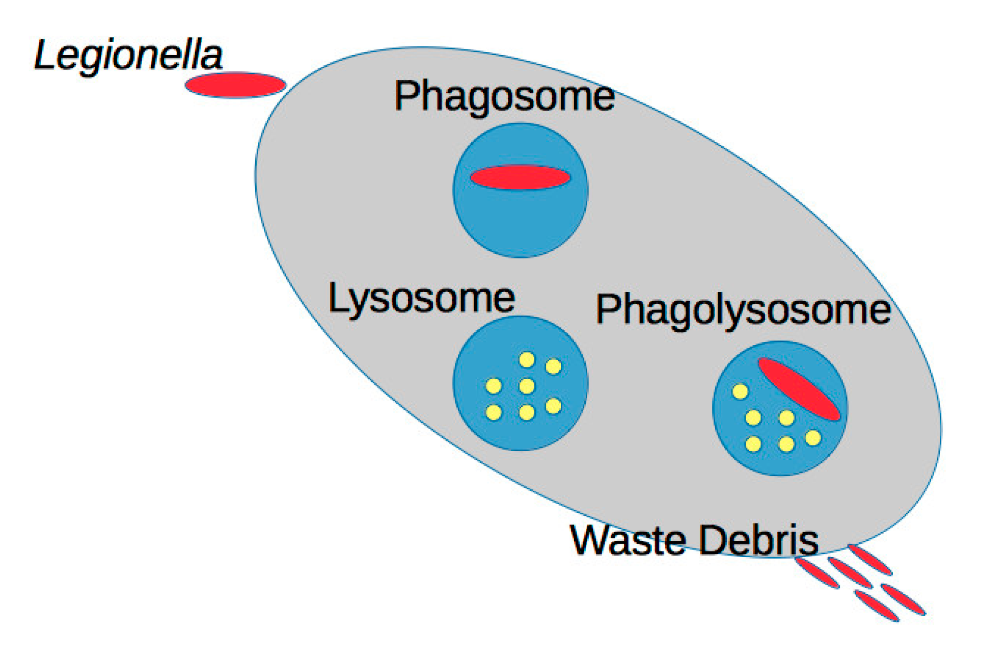
How L. pneumophila grows in the human body impacts therapeutic options, thus having a further public health impact. The human body has evolutionarily conserved cells (neutrophils) that serve as sentry cells to protect the body from hazards. The alveolar macrophage (AMac) is one such neutrophil and is the infectious location of L. pneumophila in the human body [17,18,19]. AMacs utilize phagocytosis (simplified in Figure 1) to internalize cells and other substrates necessary during their lifecycle. However, due to its intracellular growth capabilities, AMacs, like other phagocytes, are a critical component in L. pneumophila’s lifecycle [20,21,22]. Once internalized in the AMac, L. pneumophila primarily uses Dot/Icm Type-IV secretion systems to modulate the capsase-1 process within the AMac. The capsase-1 process is intended to limit the growth and proliferation of organisms intracellularly absorbed into the AMac [22,23]. The primary result of modulating the capsase-1 process is the prevention of lysosome-phagosome fusion, which the phagocyte uses to digest the internalized cell. This is just one of a set of biochemical processes that are used to halt the phagocytosis process allowing for proliferation of the pathogen. Space and scope do not allow for a full discussion of the pathogenesis; however, excellent resources are recommended to expand upon this brief synopsis [1,18,19,22,23,24].

During the pathogenesis process, L. pneumophila can then exit the host-cell (AMac) with or without apoptosis or lysis. Once externalized, L. pneumophila then attracts another phagocyte and continues proliferating, resulting in the rapid body burden that is typical of LD [25]. This rapid body burden is why therapeutics and recovery from LD are challenging. Therefore, controlling or eliminating exposure to L. pneumophila is crucial to protect public health.

1.3. Health Effects Within Diverse Populations Are Not Equal

Most infectious disease outcomes are heterogeneous within diverse populations. When examining demographic trends in LD cases for the USA, consistent outcomes are noted. The elderly, males, smokers, and African Americans are the demographic groups with the greatest caseloads [13,14]. Contrastingly to other infectious disease hazards, the young represent the lowest number of cases [13]. It is important to note that it is often tempting to combine this to say that African American elderly males are at the greatest risk. However, this confounds the epidemiological evidence since each of these demographic groups were analyzed separately, and not in combination, for example, only males and only elderly, not elderly males. Secondly, this conflates risk and caseloads, as caseloads are the realization of an estimated risk of infection and illness. Due to the heterogeneity in health outcomes, a risk model to target public health interventions for a population needs to consider this heterogeneity.

1.4. QMRA Can Optimize L. pneumophila Interventions

Quantitative microbial risk assessment (QMRA) is a computational science that allows for the analysis and forecasting of pathogenic health risks [26]. QMRA has demonstrated its capabilities as an analytical and decision support science in multiple environmental media and exposure scenarios [27,28,29,30]. Subsequently, QMRA can bridge the practitioner divide between environmental engineering and environmental health sciences. This bridge between fields is vital to improve targeted public health protection with the use of engineering controls. For example, in Hamilton et al. (2019) [31], QMRA modeling was used to estimate critical L. pneumophila concentrations for sets of health targets. Narrowing this gap between environmental engineering and environmental health sciences leads to more targeted and effective public health interventions moving forward.

1.5. Current QMRA Modeling Methods Are Inadequate for L. pneumophila

In QMRA modeling, to account for within-group heterogeneity, a group-specific exposure volume—for example, elderly inhalation volume for elderly hospital patients—is used to make the exposure model specific to that group. This method has been employed the most in recreational water QMRA models since children’s recreational risks are often used to prioritize intervention options [28,32,33,34]. Therefore, for host-age heterogeneity in L. pneumophila exposure modeling, inhalation volumes for children, adults, and the elderly can be chosen from the EPA exposure factors handbook [35] to make the exposure model specific to the population’s age heterogeneity. The concept is that once the exposure volume has been adapted to the specific age group, then the dose will be descriptive to that age group, then, in turn, the modeled risk will be descriptive to that group. In drinking water systems, particularly for opportunistic pathogens, the delineation of risks based on the demographics of the population is noted as a necessary component with the same underlying method used or recommended [8,15,26,29,36,37,38].

Unfortunately, due to limitations in the dose-response model derivation, this current method of altering group-specific exposure factors will produce risk estimates that are inaccurate when compared to the known clinical outcomes for humans exposed to pathogens such as L. pneumophila. Due, in part, to nearly identical respiration rates between the elderly and adult populations [35], the exposure factor adjustment method results in equivalent probabilities of infection. This is not considered an issue until the probability of illness is calculated using either the morbidity ratio, conditional dose-response, or probability of illness dose-response. In any of these methods, to estimate the probability of illness or disease outcome, the equivalence of risk estimates remains due to a fundamental limitation of the mechanistic dose-response models.

The microbial dose-response model derivation (simplified in Equation (1)) implicitly assumes host susceptibility homogeneity when considering the probability of infection, when these models are used to model the probability of illness or disease endpoint, this host homogeneity assumption remains. The mechanistic dose-response models’ derivation is described in greater detail elsewhere; however, a simplified version will be presented here [26,38,39].

$$\begin{array}{cccc}p\left(d\right)=& {\displaystyle \sum _{k=k_{min}}^{\infty }}\frac{{\left(d·r\right)}^2{e}^{-d·r}}{k!}& {\displaystyle \sum _{j=k}^{\infty }}\frac{d{\left(1-r\right)}^{j-k}{e}^{-d\left(1-r\right)}}{\left(j-k\right)!}& \\ & \hfill p\left(d\right)=& {\displaystyle \sum _{k=k_{min}}^{\infty }}\frac{{\left(d·r\right)}^2{e}^{-d·r}}{k!}\cong & p\left(d\right)=1-\exp \left(-r·d\right)\end{array}$$

(1)

The mechanistic microbial dose-response models are derived from the same set of three first principles that we can track through Equation (1):

• The host is exposed to an average dose in the environment (d), modeled as a random discrete Poisson dose (red in Equation (1)).
• From this d, there are j pathogens that are delivered to a susceptible location within the host, for example, alveoli for L. pneumophila.
• From those j organisms, k survive to initiate an infection, which is a Boolean outcome and, thus, the binomial distribution (blue in Equation (1)). These likelihoods are coupled to develop the joint probability that d will result in an infection, which is then simplified to the exponential dose-response function at the far right (green in Equation (1)).

The simplicity of this derivation allows the mechanistic dose-response models to be used across a wide range of host and pathogen species and exposure routes. However, it is not possible to model host effects, such as age, physiology, or immune response in the standard dose-response models. Since probability of illness dose-response models retain this derivational limitation, this same implicit assumption of host homogeneity exists. For only a small number of pathogens, where appropriate data were garnered from literature reviews, host-side dynamics have been included in dose-response models [40,41,42]. However, these data for such advanced dose-response models are expensive and difficult to develop. Thus, this research was targeted at developing a means of describing host heterogeneity outside of the dose-response models, until these host heterogeneity dose-response models can be developed.

1.6. Scope and Purpose of Research

Through this research, we have developed a method to model the risk of illness and specific health effects for different age, sex, and racial groups within diverse populations. Once the probability of illness is accurately modeled, then severe disability-adjusted life years (DALYs) are used to estimate the risk of LD and moderate DALYs for Pontiac fever. This resolution in the QMRA model is vital to target realistic public health interventions within diverse populations. The method developed in this research is targeted to modeling a demographic-specific morbidity ratio using surveillance data from the CDC. This will allow for the estimation of a probability of illness for a specific demographic group with greater accuracy than possible under current QMRA methods.

Since the QMRA methodology is scenario dependent, we have developed this QMRA model to address a heterogeneous population comprised of a mixture of races and sexes and ages. Total numbers of each group are not pertinent since we will only be comparing the general daily risks and DALYs, not estimating the likely numbers of cases. The scenario is the use of a shower (length of shower is a model variable), where there is an uncertain concentration of L. pneumophila in the premise plumbing water.

2. Modeling Methods

This research is developed in two stages. The first stage develops a stochastic simulation to estimate the risk of infection since the dose-response model available estimates the probability of infection [43]. The second stage is the development of the new method to model the probability of illness and DALYs for the heterogeneous population. For the first stage, the probability of infection is modeled for broad age ranges: children (0–18 years), adults (19–60), and the elderly (≥60). This will facilitate the evaluation of the improvement in model accuracy using the new method. Further, when conducting a simulation using random variates, it is important to conduct the appropriate quality assurance tests to ensure that a random sample is truly random. Ross (2007) [44] has a good description of this.

2.1. Two-Dimensional Simulation for Risk Modeling

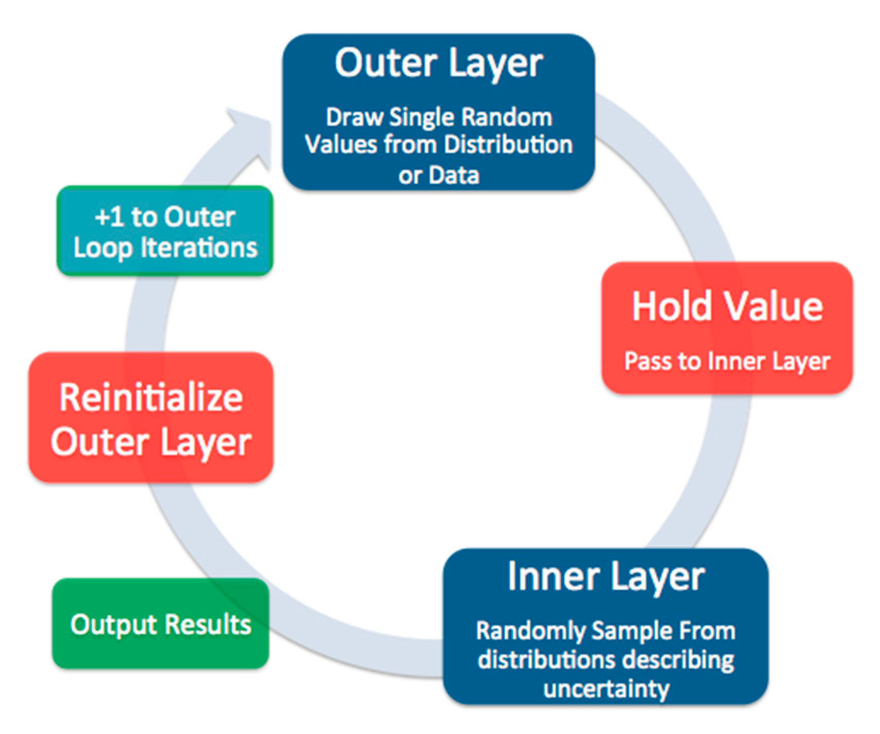
Due to the uncertainty and variability in the model variables and outputs, the two-dimensional Monte Carlo (2D-simulation) method is used. Two-dimensional-simulation modeling is an effective method of accounting for both variability and uncertainty in a model [45]. By sampling variable and uncertain variables at different levels, uncertainty in the simulation can be accounted for with greater confidence. Figure 2 shows a conceptual diagram of the 2D-simulation, where variables with variability (variable variables) are sampled in the outer layer, and uncertain variables (variables with uncertainty) are sampled in the inner layer. This invokes the law of large numbers for each outer layer iteration. Thus, resulting in computational data with an n of 1001 for variable variables and 10,010,000 for uncertain variables. Variable variables and uncertain variables are randomly sampled from the probability distributions assigned to them (

Table 1. Parameters, distributions used, and distribution parameters of the Pinf model.

Model Parameter	Distribution Variability or Uncertainty a; AICw	Value(s)	Units	Citation
Hmix	Truncated Normal b—V AICw = 0.350	µ c = 0.5778; σ d = 0.0399 UB e = 0.5094; LB f = 0.6472	Unitless	Estimated in this research
Cmix	Cauchy—V AICw = 0.65	Location = 0.363; Scale = 0.0217
AFQ1H	Triangular—V AICw = NA h	Min = 0.0097; Median = 0.0013 Max = 0.0069		Distribution optimized in this research, data used for optimization from [46]
AFQ2H	Triangular—V AICw = NA h	Min = 0.0014; Median = 0.0027 Max = 0.0128
AFQ3H	Triangular—V AICw = NA h	Min = 0.0010; Median = 0.0015 Max = 0.0061
AFQ1C	Truncated Weibull—V AICw = 0.349	Scale = 2.754; shape = 0.0308 UB = 0.0478; LB = 1(10−15)
AFQ2C	Truncated Weibull—V AICw = 0.460	Scale = 4.125; shape = 0.0373 UB = 0.0473; LB = 1(10−15)
AFQ3C	Triangular—V AICw = NA h	Min = 0.0097; Median = 0.0128 Max = 0.0173
Cw	Uniform—U AICw = NA h	Min = 1; Max = 1(106)	CFU L−1	Min [47], Max [48]
PC	Uniform—V AICw = NA h	Min = 0.25; Max = 0.65	Unitless	Value from [29]
ts	Uniform—V AICw = NA h	Min = 0.0333; Max = 0.25	Hours	Estimated in this research
RI,Child	Triangular—V AICw = NA h	Min = 0.0076; Median = 0.0111 Max = 0.013	m3 h−1	Distributions chosen in this research, data from US EPA exposure factors handbook [35]
RI,Adult	Triangular—V AICw = NA h	Min = 0.012; Median = 0.0124 Max = 0.013
RI,Elderly	Point value—V AICw = NA h	0.012
DF1	Truncated Logistic b—U AICw = 0.525	Location = 0.06777; Scale = 0.04305 UB = 0.01; LB = 0.195	Unitless	Distributions from this research, data from [49]
DF2	Truncated Weibull b—U AICw = 0.658	Scale = 0.4134; shape = 0.2102 UB = 0.00; LB = 0.41
DF3	Truncated lognormal b—U AICw = 0.429	µ = –1.052; σ = 0.4350 UB = 0.159; LB = 0.62
k	Triangular—U AICw = NA h	Median = 0.00599; Min = 0.00326; Max = 0.131		Distribution from this research. Values from [43]
$\widehat{M{R}_C}$;$\widehat{M{R}_A}$;$\widehat{M{R}_E}$g	Point values AICw = NA h	0.0077; 0.097; 0.75 for Child Adult and Elderly respectively		Calculated in this research Data from [50]
$\widehat{M{R}_{AI}}$;$\widehat{M{R}_A}$;$\widehat{M{R}_B}$;$\widehat{M{R}_W}$;$\widehat{M{R}_O}$g	Point values AICw = NA h	0.0025; 0.010; 0.15; 0.61; 1.4 (10−5) for American Indian; Asian; Black; White and Other races respectively
$\widehat{M{R}_M}$;$\widehat{M{R}_F}$g	Point Values AICw = NA h	0.64; 0.36 for male and female respectively
DWM	Triangular—U AICw = NA h	Min = 0.039; median = 0.051; max = 0.06		Distributions from this research data from [51]
DWP	Triangular—U AICw = NA h	Min = 0.104; median = 0.125; max = 0.152
DWS	Triangular—U AICw = NA h	Min = 0.179; median = 0.217; max = 0.251

^a—V = Variability, U = Uncertainty, ^b—necessary to ensure no negative values, while using the distribution that best fit the data; ^c—µ = mean; ^d—σ = standard deviation; ^e—UB = Upper Bound; ^f—LB = Lower Bound; min = minimum; max = maximum; ^g—Corrected for population; ^h—AICw is not applicable for assumed distributions or point values.

). This research uses random sampling as opposed to one that is managed using a technique, such as the Latin hypercube, to ensure stochasticity using a seed of 36 (required for reproducible stochastic models). The 2D-simulation and all subsequent analyses and plotting were programmed in R (version 3.5.3 “Eggshell Igloo”; R Core Team, Vienna, Austria.). All statistical inferences were performed using the analysis of variance (ANOVA) with an alpha of 0.05. Because there are 10,010,000 computational data points of estimated risks, the central limit is overcome and negates the need for normality tests.

Since the Monte Carlo method uses probability distributions to describe model variables and parameters, these distributions either need to be optimized to data or carefully assumed [44,52]. This research assigns uniform or triangular distributions as assumed distributions. These distributions do not impose a detailed shape or underlying assumption of the functions. These distributions are parameterized to available descriptive statistics such as minimum, maximum, and likeliest value.

For those variables, where enough data (greater than 10 data points) is obtained, probability distributions are optimized to these data using the optim function in R. This function uses the Nelder-Mead algorithm to converge to the global minimum of the log-likelihood function. To determine the best fitting distribution, the Akaike Information Criterion weights (AICw) are used. The AICw discounts for the number of parameters in the optimized model, thus, making for a more even comparison between optimized models. AICw values for the best performing distributions can be found in Table 1; all continuous probability distributions available in R were optimized.

2.2. Exposure Model and Probability of Infection

An aerosol size small enough (≤5 µm) to allow for inhalation into the lung is required for at-risk exposure to L. pneumophila to result in any change of infection. Outbreak data implicates showers as the activity most associated with use patterns, aerosol generation/exposure, and LD illnesses. Additional studies corroborate that showers also produce the highest level of contained aerosolized particles on a consistent basis [6,24,29,53]. Therefore, the exposure model must account for the following:

• Concentration of L. pneumophila in the premise plumbing water;
• Concentration of L. pneumophila in the air during showering, within a shower duration;
• Generation of aerosols sized ≤5 µm;
• Delivered dose to alveoli of human lungs, accounting for intermediate losses in the previous two regions of the respiratory system.

Using an environmental chamber configured as a shower, Zhou et al., (2007) [46] investigated the generation and size distribution of drinking water aerosols. Their study examined three separate flow rates and two temperature ranges, 24–25 °C for cold water and 43–44 °C for hot water [46].

Equation (2) uses the Zhou et al. (2007) data to model AF_Qx, which is the fraction of aerosols that are ≤5 µm, generated after mixing hot and cold water at flow rate x. This is performed using fractional proportions of 43 °C water for hot water and 24 °C for cold water. This models the aerosol fractions for each flow rate and each broad temperature classification, where AF_QxC and AF_QxH are the cold and hot water aerosol fractions for each flow rate x (5.1, 6.6, and 9.0 L min⁻¹), respectively. This level of granularity of the aerosolization has not been included in a QMRA previously; therefore, these data were chosen to provide for this option.

However, people do not shower in only cold or hot water; therefore, warm water needs to be modeled. Equation (2) uses cold and hot water mixtures, C_mix and H_mix, which are fractional portions of cold and hot water used to develop a safe and comfortable showering temperature. The mixed water temperature modeled is monitored to ensure that it does not exceed 43 °C to prevent scalding [54]. Distributions for C_mix and H_mix were chosen by iteratively solving for each mixture value (C_mix and H_mix) at each temperature setting for an upper value of 43 °C and a low value of 30 °C, using 0.5 °C increments. Then probability distributions are optimized to the iteratively solved mixture values (AICw in Table 1). Distributions and parameter values for AF_QxC, AF_QxH, C_mix, and H_mix can be seen in Table 1.

$$A{F}_{Qx}=\left(H_{mix}·A{F}_{QxH}\right)+\left(C_{mix}·A{F}_{QxC}\right)$$

(2)

Equation (3) uses AF_QX estimates to model the concentration of L. pneumophila in the air within aerosols ≤5 µm aerosols. For Equation (3), the variability of concentration in the water (C_w) is modeled as a uniform distribution parameterized from the open literature [47,48]. The concentration of L. pneumophila in these studies is serogroup-1 and based on a culture method [47,48]. L. pneumophila concentrations vary greatly in municipal water, and a QMRA model developed for the real world uses site-specific sampling results to inform the concentration. This model is intended as a generalized risk model rather than a model for a specific municipality or region. Thus, as in all QMRA models, the values used in the distributions should not be used for a policy or engineering application but rather for the method used. Then, a partitioning coefficient (PC) allows the estimation of L. pneumophila concentration in the air during a shower (C_aQx; Table 1).

$$C_{aQx}=C_w·PC·A{F}_{Qx}$$

(3)

To model the dose delivered to the alveoli, three compartment models are operated in series using the three-region lung model [49]. Equation (4) models the inhalation of the aerosols generated in the shower. The concentration in the air (region-0) is converted to a dose inhaled into the respiratory system ($D_{R_{0}Qx}$) for shower flow rate x. Then, shower duration (t_s) and the inhalation rate dependent on age group (R_I,age; normalized to t_s) models $D_{R_{0}Qx}$.

$$D_{R_{0}Qx}=C_{aQx}·t_s·R_{I,age}$$

(4)

Equation (5) models the dose lost to region-1 of the respiratory system for flow rate x ($D_{R_{1}Qx}$), using the deposition fraction in region-1 (DF₁; Table 1). The $D_{R_{1}Qx}$ estimates and deposition fraction for region-2 (DF₂; Table 1) by modeling the dose lost to region-2 at flow rate x ($D_{R_{2}Qx}$; Equation (6)). Equation (7) uses these previous results from Equations (4–6) to model the dose to the alveolated region of the lungs at flow rate x ($D_{R_{3}Qx}$) using the deposition fraction for region-3 (DF₃; Table 1). $D_{R_{3}Qx}$ is the dose that deposits within the alveoli, which is the dose that is used to estimate the risk of infection for flow rate x (P_{inf, x}). The deposition fractions used are from a standard text used throughout inhalation toxicology as well as QMRA modeling [30,55]. P_{inf, x} is modeled using Equation (8), the exponential dose-response model (Equation (8)). The exponential has one parameter k (Table 1), where k is the probability of a pathogen surviving to initiate an infection in the host [26].

$$D_{R_{1}Qx}=D_{R_{0}Qx}·D{F}_1$$

(5)

$$D_{R_{2}Qx}=\left(D_{R_{0}Qx}-D_{R_{1}Qx}\right)·D{F}_2$$

(6)

$$D_{R_{3}Qx}=\left[D_{R_{0}Qx}-\left(D_{R_{1}Qx}+D_{R_{2}Qx}\right)\right]·D{F}_3$$

(7)

$$P_{{\inf }_x}=1-\exp \left(-k·D_{R_{3}Qx}\right)$$

(8)

2.3. Risk Characterization: Probability of Illness and DALYs

The data from the morbidity and mortality weekly report (MMWR) for racial and gender incidence rates are not age-adjusted [13]. Therefore, before calculating the probability of illness and DALYs for the demographic groups, the groups’ risk estimates must be combined into an overall population risk. Equation (9) is an expansion of the inclusion/exclusion principle of a union, which can be used to combine the probability of infection estimates for all ages (children, adults, and the elderly) at flow rate x (${R_E}_x$ in Equation (9)) [30]. Once P(${R_E}_x$) is modeled, the probability of illness can be estimated using this research’s new method.

$$P_{R_x}=\left|{\displaystyle \bigcup }_{i=1}^n{R}_i\right|={\displaystyle \sum }_{j=1}^n{\left(-1\right)}^{j+1}\left({\displaystyle \sum }_{1\le i_1\le \dots \le i_j\le n}\left|R_i\cap \dots \cap R_{i_j}\right|\right)$$

(9)

2.4. Method to Estimate Morbidity Ratio Proxies and Dynamic Health Effect QMRA Models

Morbidity ratios are often used to model the probability of illness (P_ill) given exposure and infection [56,57]. Using data from the morbidity and mortality weekly report (MMWR) [13], the incidence rate for each demographic group is used to calculate a morbidity ratio proxy for that group ($\widehat{M{R}_G}$). This will allow for the P_ill to be modeled for each group and overcome the assumed homogeneity of health effects from the dose-response model derivation.

The method for estimating $\widehat{M{R}_G}$ for each of the demographic groups is founded on concepts of utilizing relative risks from incidence rates. Using Equation (10), $\widehat{M{R}_G}$ can be estimated using the national attack rate (AR) or incidence proportion of 0.05 [58], legionellosis incidence rate for the demographic group (IR_G) from the MMWR [59], and the legionellosis incidence rate for the total US population (IR_P) during the years of the MMWR study. All $\widehat{M{R}_G}$ values can be seen in Table 1. A brief logic explanation is provided in the supplementary material.

$$\widehat{M{R}_G}=AR·\frac{I{R}_G}{I{R}_P}$$

(10)

Using $\widehat{M{R}_G}$, the probability of illness given exposure and infection for each demographic group at flow rate x ($P_{ill,G_x}$) is estimated using Equation (11). Equation (11) estimates P_ill,G for the following groups: children (P_ill,C), adults (P_ill,A), Elderly (P_ill,E), American Indians (P_ill,AI), Asian (P_ill,Asian), Black (P_ill,B), White (P_ill,W), Other race (P_ill,O), females (P_ill,F), and males (P_ill,M).

$$P_{ill,G_x}=P_{R_x}·\widehat{M{R}_G}$$

(11)

Once the $P_{ill,G_x}$ is estimated the disability-adjusted life years (DALYs) can be estimated for each demographic group at flow rate x. For improved intervention assessment separating moderate, severe and post-acute DALYs for flow rate x ($DAL{Y}_{M_x}$, $DAL{Y}_{S_x}$ and $DAL{Y}_{P_x},$ respectively) is needed. This is postulated as a means of modeling Pontiac Fever ($DAL{Y}_{M_x}$), LD ($DAL{Y}_{S_x}$_S) and sequela from LD ($DAL{Y}_{P_x}$) at flow rate x utilizing the associated disability weights published by the World Health Organization. Equation (13) multiplies the annualized risks from Equation (12) (P_ill,G,A) by the disability weights for moderate illness, DW_M, or severe DW_S (termed DW_a in Equation (12)). The value of $DAL{Y}_{P_x}$ is estimated using Equation (14) to account for post-acute illness (DW_P) and DW_S disability weights. DWs is used in Equation (14) since post-acute is estimating sequela for survivors of LD.

$$P_{ill,G,A}=1-{\displaystyle \prod }_1^j\left(1-P_{ill,G_x}\right)$$

(12)

$$DAL{Y}_{a_x}=P_{ill,G,A}·D{W}_a$$

(13)

$$DAL{Y}_{P_x}=P_{ill,G,A}·\sum \left(D{W}_P,D{W}_S\right)$$

(14)

3. Results

Due to space considerations, the 5.1 L min⁻¹ flow rate will be used to demonstrate the results. The plots depict the same fundamental trends for the other two flow rates, 6.6 and 9.0 L min⁻¹. Results of the statistical comparisons across flow rates using the ANOVA are presented below. All plots for the other two flow rates can be seen in the supplementary information. Full model plotting and analysis source code are available in the supplementary information.

3.1. Effects of Flow Rate

With a p-value of 1 (10⁻⁵), there is a significant difference between the first two flow rates (5.1 and 6.6 L min⁻¹) when comparing the probability of illness. There is also a significant difference in probability of illness or DALY between the lowest and highest, 5.1 and 9 L min⁻¹ p-value of 1 (10⁻⁴), and medium and highest 6.6 and 9.0 L min⁻¹, p-value of 1 (10⁻⁵). With higher flow rates, there is an increased concentration of aerosolized L. pneumophila in the shower air resulting in higher inhalation doses, thereby higher risks.

3.2. Age Demographic Risks

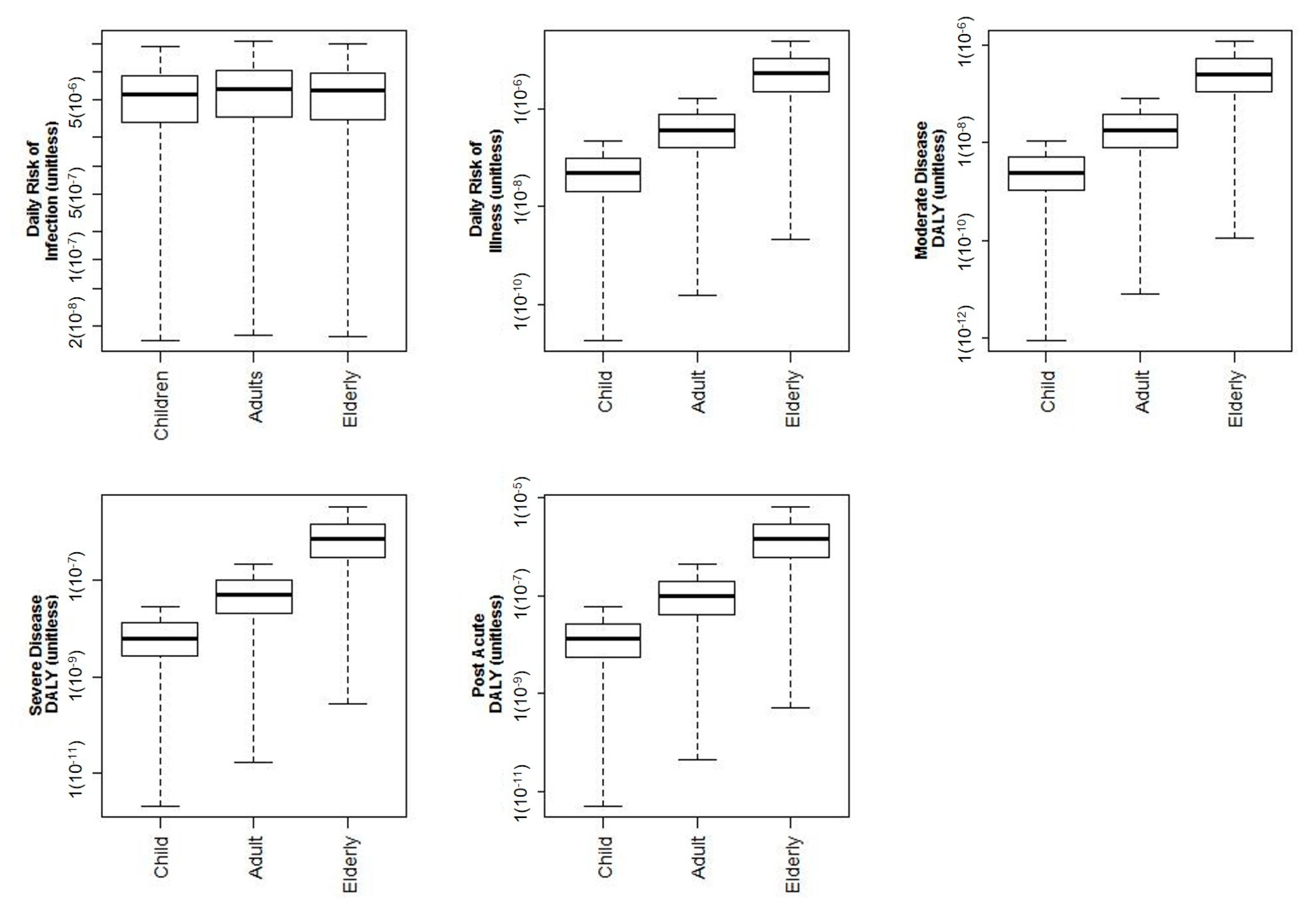
Risk results were compiled into boxplots for the presentation of the results and ease of comparison between groups. All the boxplots are visualizing the natural log of the risks to allow for improved visualization. Age demographic risk results can be seen in

Table 2. Risk model results for each demographic set for flow 5.1 L min⁻¹.

Demographic Group	Statistic	Pinf a	Pill b	MDALY c	SDALY d	PDALY e
Child	U95 f	7.29 (10−6)	2.39 (10−7)	1.20 (10−8)	3.03 (10−8)	6.36 (10−8)
	M g	2.61 (10−6)	4.98 (10−8)	2.48 (10−9)	6.28 (10−9)	1.32 (10−8)
	L95 h	2.69 (10−7)	4.19 (10−9)	2.08 (10−10)	5.28 (10−10)	1.11 (10−9)
Adult	U95	7.93 (10−6)	1.84 (10−6)	9.30 (10−8)	2.36 (10−6)	4.88 (10−7)
	M	2.84 (10−6)	3.85 (10−7)	1.91 (10−8)	4.87 (10−8)	1.02 (10−7)
	L95	2.93 (10−7)	3.24 (10−8)	1.60 (10−9)	4.09 (10−9)	8.53 (10−9)
Elderly	U95	7.57 (10−6)	2.64 (10−5)	1.33 (10−6)	3.37 (10−6)	7.00 (10−6)
	M	2.71 (10−6)	5.54 (10−6)	2.75 (10−7)	7.03 (10−7)	1.47 (10−6)
	L95	2.79 (10−7)	4.65 (10−7)	2.30 (10−8)	5.88 (10−8)	1.23 (10−7)
Combined Ages	U95	5.95 (10−5)	Not Modeled j
	M	1.25 (10−5)
	L95	1.05 (10−6)
American Indian	U95	NA i	8.34 (10−6)	4.20 (10−7)	1.07 (10−6)	2.21 (10−6)
	M		1.75 (10−6)	8.70 (10−8)	2.21 (10−7)	4.65 (10−7)
	L95		1.47 (10−7)	7.27 (10−9)	1.86 (10−8)	3.91 (10−8)
Asian	U95		5.56 (10−6)	2.80 (10−7)	7.05 (10−7)	1.48 (10−6)
	M		1.16 (10−6)	5.78 (10−8)	1.48 (10−7)	3.09 (10−7)
	L95		9.80 (10−8)	4.86 (10−9)	1.24 (10−8)	2.60 (10−8)
Black	U95		3.45 (10−5)	1.74 (10−6)	4.9 (10−6)	9.19 (10−6)
	M		7.24 (10−6)	3.63 (10−7)	9.15 (10−7)	1.92 (10−6)
	L95		6.09 (10−7)	3.04 (10−8)	7.68 (10−8)	1.62 (10−7)
White	U95		2.34 (10−5)	1.71 (10−6)	2.97 (10−6)	6.20 (10−6)
	M		4.91 (10−6)	2.45 (10−7)	6.21 (10−7)	1.30 (10−6)
	L95		4.13 (10−7)	2.04 (10−8)	5.21 (10−8)	1.10 (10−7)
Other	U95		1.48 (10−7)	7.38 (10−9)	1.87 (10−8)	3.93 (10−8)
	M		3.10 (10−8)	1.55 (10−9)	3.91 (10−9)	8.22 (10−9)
	L95		2.61 (10−9)	1.30 (10−10)	3.29 (10−10)	6.90 (10−10)
Female	U95		2.10 (10−5)	1.06 (10−6)	2.69 (10−6)	5.61 (10−6)
	M		4.41 (10−6)	2.19 (10−7)	5.59 (10−7)	1.17 (10−6)
	L95		3.71 (10−7)	1.84 (10−8)	4.69 (10−8)	9.80 (10−8)
Male	U95		3.85 (10−5)	1.92 (10−6)	4.93 (10−6)	1.02 (10−5)
	M		8.07 (10−6)	4.03 (10−7)	1.02 (10−6)	2.14 (10−6)
	L95		6.79 (10−7)	3.37 (10−8)	8.56 (10−8)	1.79 (10−7)

^a—Probability of infection; ^b—Probability of illness; ^c—Moderate disability-adjusted life years (DALY) (Pontiac Fever); ^d—Severe DALY (Legionaries’ Disease); ^e—Post Acute DALY; ^f—Upper 95th Percentile; ^g—Median; ^h—Lower 95th Percentile; ⁱ—Combined Ages Pinf using equation 8 used; ^j—due to data from MMWR not age-adjusted.

and Figure 3.

As can be seen, and as discussed previously, modeling the probability of infection does not represent realistic population impacts. The risk of infection incorrectly assesses equivalent risks to adults and the elderly. This is due to the similarity of respiration volumes for these groups.

When the new method is used to model the probability of illness for the elderly population, these risks are higher than the other age groups (Figure 3). This follows through to a higher burden of disease using DALYs for the moderate illness (MDALY), from Pontiac Fever, post-acute illness DALY (PDALY), and severe illness (SDALY). When modeling infection, there is no significant difference between ages—ANOVA p = 0.12. When modeling P_ill and DALY, there is a significant difference between ages for probability of illness—p = 4 (10⁻⁴), PDALY—p = 3 (10⁻⁴), SDALY—p = 3 (10⁻⁴), and MDALY—p = 4 (10⁻⁴).

3.3. Race Demographic Risks

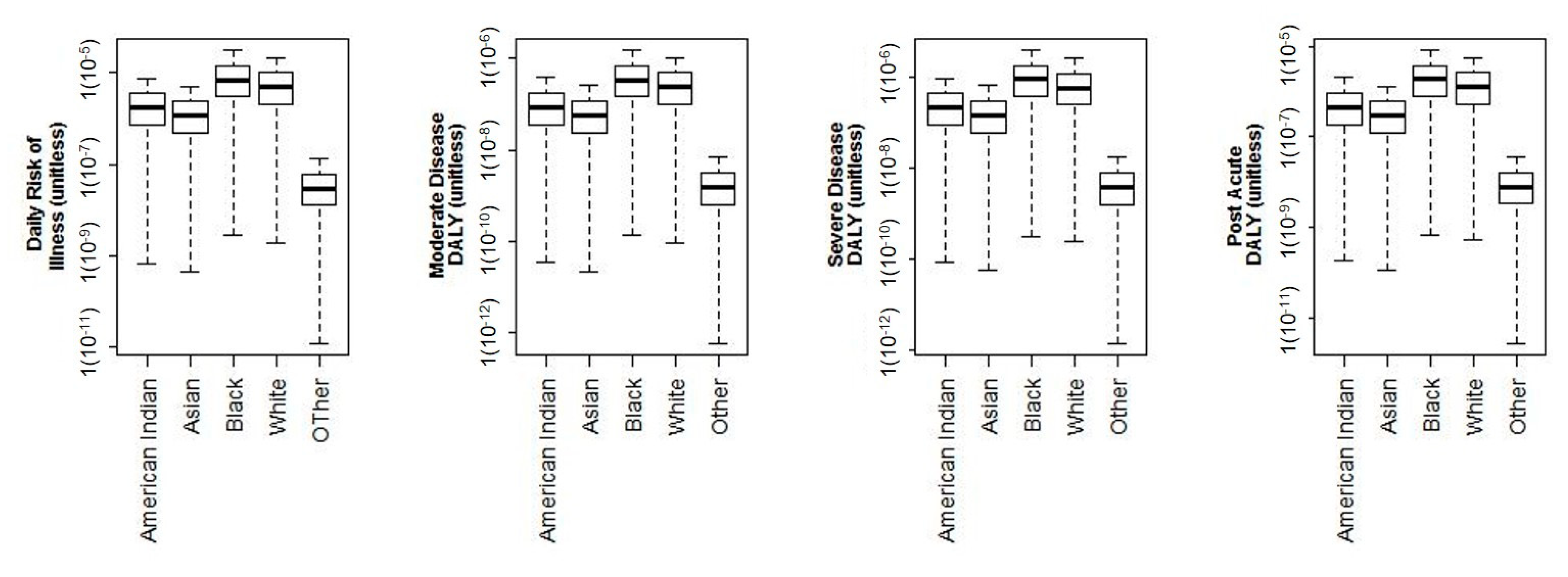
Racial demographics were modeled for American Indian, Asian, Black, White, and Other racial demographics. Figure 4 shows the risks of illness and DALYs for each of the racial demographic groups. There is a significant difference between Black and Asian risks—p = 3 (10⁻⁴), Black and Other risks—p = 5 (10⁻⁵), Black and White risks—p = 1 (10⁻³), and White and Other risks—p = 1 (10⁻⁵).

3.4. Sex Demographic Risks

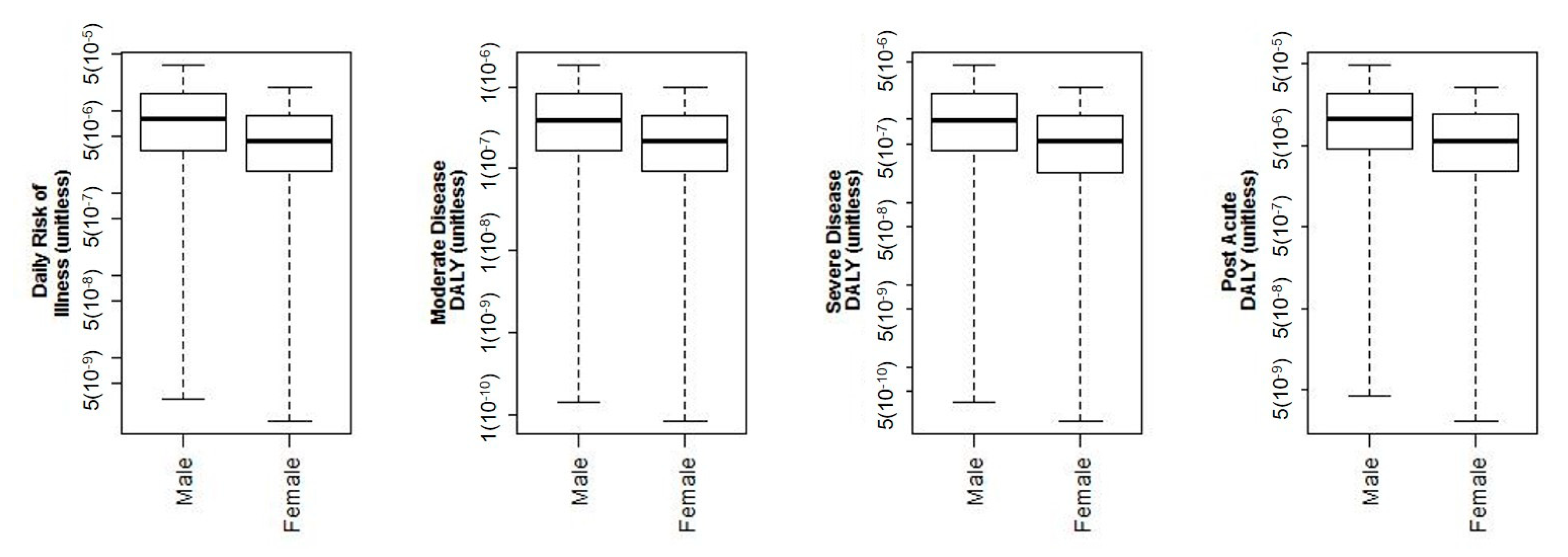
Risk results for the sex demographics can be seen in Figure 5. The male population has increased risk of severe and post-acute DALYs as compared to the female population. This is also representative of known clinical manifestations of legionellosis since men have more frequent illnesses and fatalities [13,24,50]. The differences between sex were statistically significant for only SDALY p = 3 (10⁻⁴) and PDALY p = 1 (10⁻³).

4. Discussion

4.1. Interpretation of Results

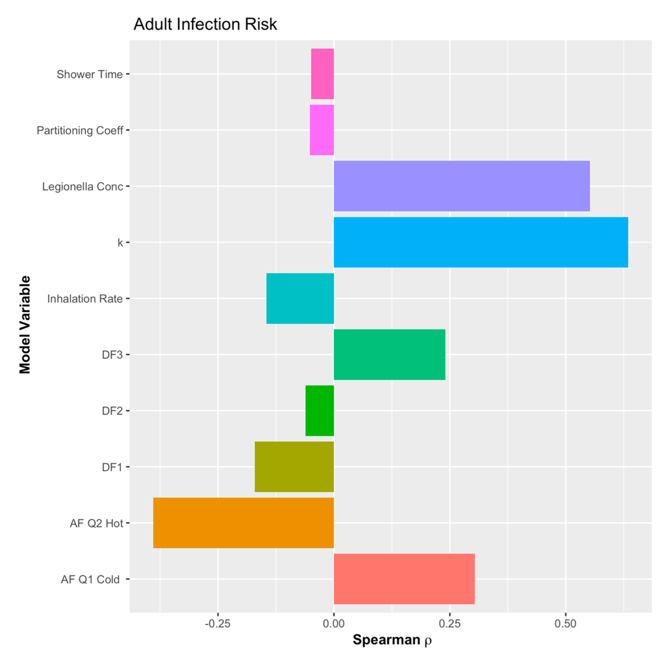
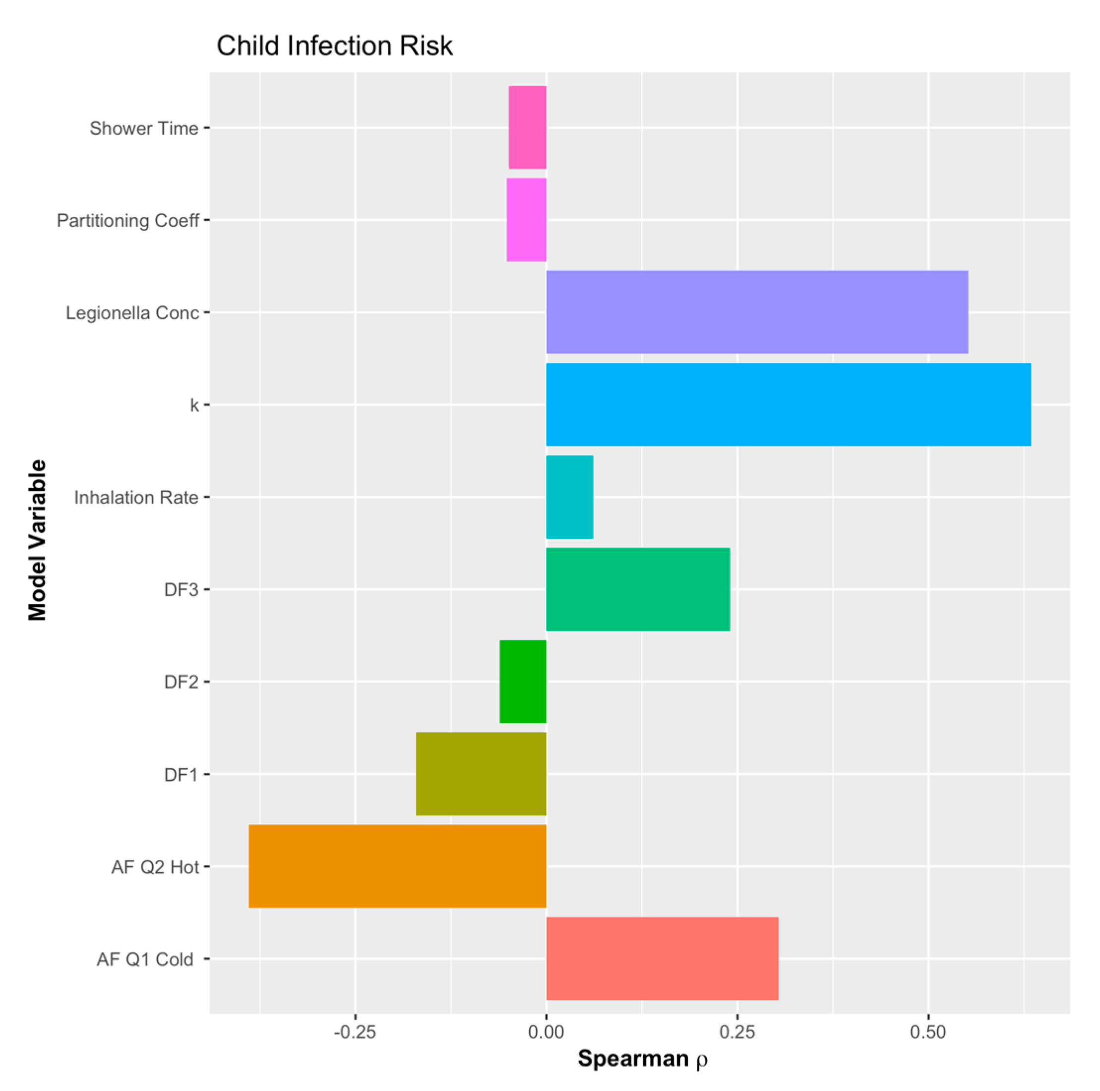
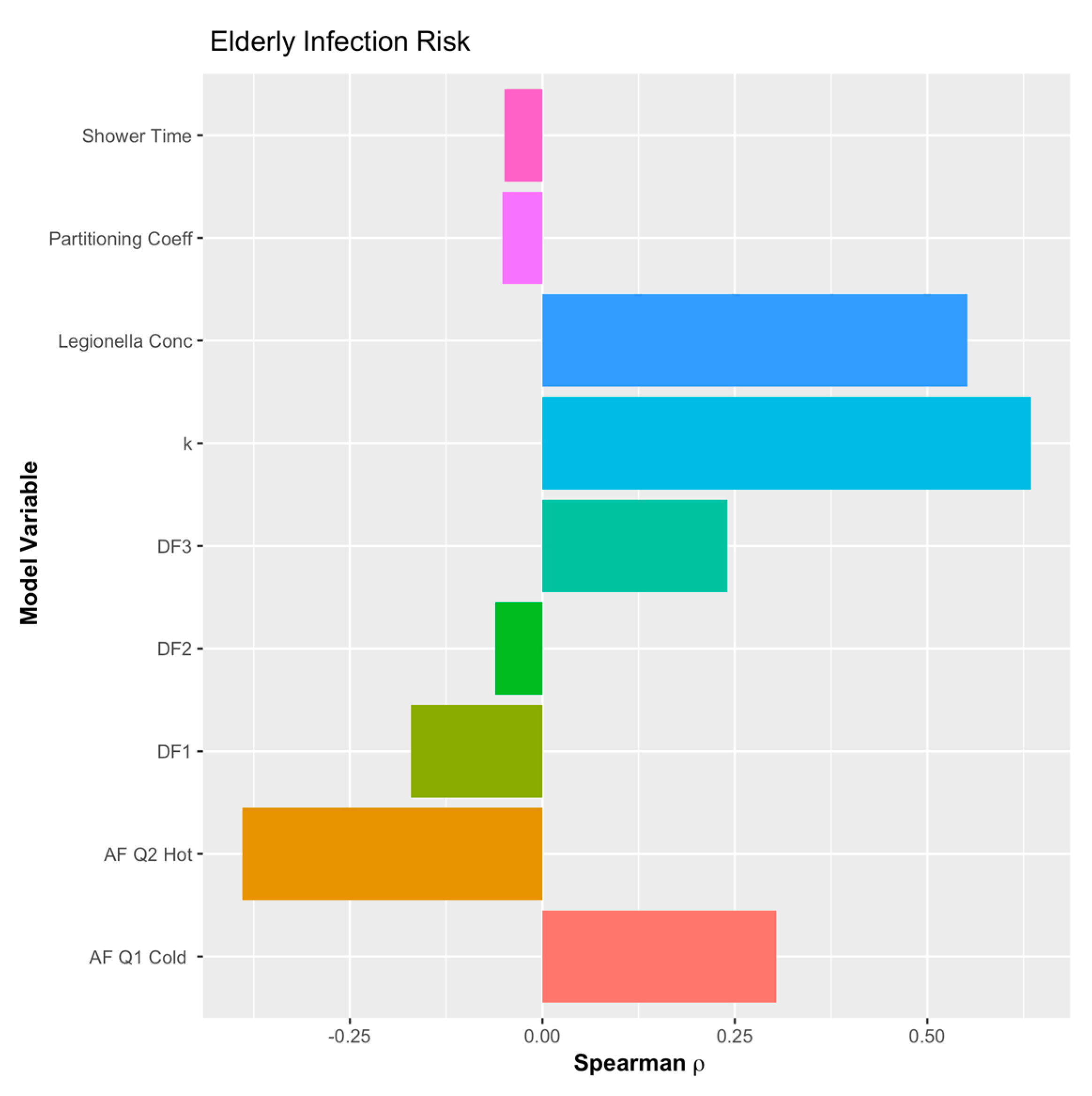
A sensitivity analysis was conducted for the example QMRA model, but the morbidity ratio proxy could not be included since it can only be estimated as a point value. Thus, without variation in the Monte Carlo simulation, it cannot be included in the sensitivity analysis. However, as can be seen in Figure 6, Figure 7 and Figure 8, the concentration of L. pneumophila in the water is the second most critical parameter in the example QMRA model, just following the exponential dose-response model parameter (k). It is also important to note that the deposition fraction within the respiratory system (DF values) demonstrate a negative impact on the estimated risks, until the third region of the lungs (DF3 in Figure 6, Figure 7 and Figure 8). This demonstrates fidelity to the reality of L. pneumophila needing to reach the alveolated third region of the lung to develop an infection in the host. The model for children demonstrates a shift from negative to lessened but positive impact from the inhalation rate variable, all the other relationships remaining the same. A sensitivity analysis for the elderly demonstrated the same impacts as adults but without an inhalation rate since that was a point value as well.

In currently used L. pneumophila QMRA models [29,31,60], risk estimations including host-age heterogeneity have not been included, quite likely due to the limitation in the dose-response model derivation that inspired this research. In this research’s QMRA model, the improvement in modeling the P_ill and DALY as compared to P_inf is highlighted best for elderly populations. The elderly population is the group best known clinically to demonstrate a significant increase in susceptibility to L. pneumophila, including the likelihood of LD and mortality. The method developed in this research derives morbidity ratio proxies to model P_ill and health outcome specific DALYs for each demographic group. This is the first instance of this level of resolution for specific demographics in QMRA modeling. This level of resolution is important to target future research towards sampling location for exposure intervention or research to explain sex and racial differences in LD risks.

A more robust method would involve a large case-control study that quantifies exposure levels to determine morbidity ratios for each of the demographic groups. Another method would be an advanced dose-response model to model the risk of illness in specific populations. These dose-response experiments would be limited to host-age and gender since only animal models could be used for L. pneumophila exposure experiments. However, as has been demonstrated in other advanced dose response models, these differences from age and other factors can be included in the mechanistic dose response models without requiring re-derivation [38,40,61]. Lastly, it may be possible to include host cell infectivity of L. pneumophila and cofactors of human illness susceptibility cofactors using an environmentally mediated transmission modeling framework [62]. The difficulty in this is like the case-control study, in that characterizing the exposures and linking them to health outcomes in the cohorts will be the most challenging aspect to model. However, by leveraging more complex methods of air transport, such as computational fluid dynamics, may provide the level of precision needed to design and operate such studies.

With regards to the source of the dose-response parameter (k), there is possible confusion over the host animal used in the dose-response experiments–guinea pigs. As was demonstrated in Bartrand et al. (2008) [62] and is discussed in greater detail in Weir 2016 [38], there is no need to adjust for host animal species. This is because the mechanistic dose-response models are derived using generalized pathogenesis principles and are derived as single-hit infection models. Therefore, so long as the host species is competent and can be infected via the same exposure route, it is a competent host species, and will not require adjustment to humans. This contrasts with toxicological dose-response modeling, where the body weight of the host must be accounted for due in major part to the toxin or toxicant needing to be digested and metabolized, from which impacts are body-size dependent. This is not the same when modeling the probability of infection since infection from a single-hit perspective is dependent on a cell being infected and allowing for the propagation of the infection.

4.2. Model Limitations

This model is limited in three primary areas. First, the model uses an approximation of the L. pneumophila concentration in premise plumbing systems. A further refined or advanced model that accounts for growth and persistence of L. pneumophila in plumbing systems will improve this substantially. Second, the development of estimates of the morbidity ratio proxy should be replaced with true morbidity ratios that are estimated from the aforementioned case-control study or replaced with an advanced dose-response model. Third, as has been discussed previously, a more complete assessment and incorporation of different susceptibility within the population can be accomplished by incorporating additional cofactors in the dose-response model. However, as also discussed, this is a first step in the improvement of Legionellosis risk estimation.

4.3. Other Potential Methods for Future Research

A method of back-calculating a probability of illness given exposure by Hamilton et al. (2017) is another possible means of modeling the probability of illness [63]. However, their method uses a very generalized assumption of non-tubercular Mycobacterium lung diseases attributable to the Mycobacterium avium complex. The underlying assumption of rates of illness for a broad set of bacterial agents presents severe limitations to the expandability of that method as well as the accuracy of the estimates from it. Furthermore, the Hamilton et al. (2017) method does not overcome the inherently assumed host homogeneity in current microbial dose-response modeling.

Another potential method to model the probability of illness is to use a mortality dose-response model. The rationale is that mortality results from severe illness. However, this still uses and potentially exacerbates the assumed homogeneity of response within hosts. Furthermore, the doses required to result in observed probabilities of mortality in controlled experiments are significantly higher than for infection, thus losing low dose resolution. This makes a QMRA model that uses such an extreme health outcome inefficient for modeling realistic interventions.

This method and the need for it highlights the fundamental limitation with current mechanistic microbial dose-response models for microbial hazards. While capable of use for multiple pathogens, exposure routes, and host species, their capabilities are limited to the simple distilled approximation of general pathogenesis. The second-generation dose response models, starting with Weir and Haas (2009), demonstrate the potential to advance the current mechanistic dose response models [40,41,64]. This gives further credence to the need for third-generation microbial dose-response models [42,65]. However, this third-generation model will require an implicit inclusion of host-side dynamics, for example, host heterogeneity, thus not solely focused on the pathogens’ ability to generate a response.

4.4. Broader Impacts of This Research

This QMRA model can be used to develop advanced risk management strategies. There is a growing interest in understanding how premise plumbing pathogens are affecting healthcare facility populations. This improved QMRA modeling method for L. pneumophila illness and DALYs will make for an ideal tool, including its capability to model specific flow rates. The importance of this capability is reinforced with the significant difference in risk outcomes between modeled flow rates. For engineers, flow rate is a critical component of plumbing design, thus broadening the use and importance of this QMRA model.

By modeling host heterogeneity, accurately using this research’s method estimates of the likelihood of health risks are more precise for the real population risks. This will make the interventions more responsive to the population members’ needs and risks. Further, in Hamilton et al. (2019) [31], critical concentrations and, thereby, reduction targets were identified using QMRA models. That QMRA model can be easily adapted using the methodology from this research to include diverse populations in the building being modeled. This will, then, also output a range of health effects to include severe, moderate, and post-acute health outcomes, previously possible. Consequently, any monitoring programs developed using this QMRA modeling methodology or monitoring results used to assess risks to the population will be more precise and representative of the population.

References

- Stout, J.E.; Rihs, J.D.; Yu, V.L. Legionella; Cianciotto, N.P., Hacker, J., Lück, P.C., Fields, B.S., Marre, R., Frosch, M., Abu Kwaik, Y., Bartlett, C., Eds.; American Society of Microbiology: Washington, DC, USA, 2002; ISBN 978-1-55581-230-0. [Google Scholar]
- CDC. Legionella (Legionnaires’ Disease and Pontiac Fever)—History, Burden and Trends. Available online: https://www.cdc.gov/legionella/about/history.html (accessed on 10 March 2019).
- Stout, J.E.; Yu, V.L.; Muraca, P.; Joly, J.; Troup, N.; Tompkins, L.S. Potable Water as a Cause of Sporadic Cases of Community-Acquired Legionnaires’ Disease. N. Engl. J. Med. 1992, 326, 151–155. [Google Scholar] [CrossRef] [PubMed] [Green Version]
- Mandel, A.S.; Sprauer, M.A.; Sniadack, D.H.; Ostroff, S.M. State Regulation of Hospital Water Temperature. Infect. Control Hosp. Epidemiol. 1993, 14, 642–645. [Google Scholar] [CrossRef] [PubMed]
- Yaslianifard, S.; Mobarez, A.M.; Fatolahzadeh, B.; Feizabadi, M.M. Colonization of hospital water systems by Legionella pneumophila, Pseudomonas aeroginosa, and Acinetobacter in ICU wards of Tehran hospitals. Indian J. Pathol. Microbiol. 2012, 55, 352–356. [Google Scholar] [PubMed]
- Tobin, J.O.; Beare, J.; Dunnill, M.S.; Fisher-Hoch, S.; French, M.; Mitchell, R.G.; Morris, P.J.; Muers, M.F. Legionnaires’ disease in a transplant unit: Isolation of the causative agent from shower baths. Lancet 1980, 2, 118–121. [Google Scholar] [CrossRef]
- Falkinham, J.O.; Pruden, A.; Edwards, M. Opportunistic Premise Plumbing Pathogens: Increasingly Important Pathogens in Drinking Water. Pathogens 2015, 4, 373–386. [Google Scholar] [CrossRef] [Green Version]
- Falkinham, J.O.; Hilborn, E.D.; Arduino, M.J.; Pruden, A.; Edwards, M.A. Epidemiology and Ecology of Opportunistic Premise Plumbing Pathogens: Legionella pneumophila, Mycobacterium avium, and Pseudomonas aeruginosa. Environ. Health Perspect. Online Res. Triangle Park 2015, 123, 749. [Google Scholar] [CrossRef] [Green Version]
- Lechevallier, M.W.; Cawthon, C.D.; Lee, R.G. Factors promoting survival of bacteria in chlorinated water supplies. Appl. Environ. Microbiol. 1988, 54, 649–654. [Google Scholar]
- Berry, D.; Xi, C.; Raskin, L. Microbial ecology of drinking water distribution systems. Curr. Opin. Biotechnol. 2006, 17, 297–302. [Google Scholar] [CrossRef]
- Pinto, A.J.; Schroeder, J.; Lunn, M.; Sloan, W.; Raskin, L. Spatial-temporal survey and occupancy-abundance modeling to predict bacterial community dynamics in the drinking water microbiome. MBio 2014, 5, e01135-14. [Google Scholar] [CrossRef] [Green Version]
- Shen, Y.; Monroy, G.L.; Derlon, N.; Janjaroen, D.; Huang, C.; Morgenroth, E.; Boppart, S.A.; Ashbolt, N.J.; Liu, W.-T.; Nguyen, T.H. Role of Biofilm Roughness and Hydrodynamic Conditions in Legionella pneumophila Adhesion to and Detachment from Simulated Drinking Water Biofilms. Environ. Sci. Technol. 2015, 49, 4274–4282. [Google Scholar] [CrossRef] [Green Version]
- Beer, K.D.; Gargano, J.W.; Roberts, V.A.; Hill, V.R.; Garrison, L.E.; Kutty, P.K.; Hilborn, E.D.; Wade, T.J.; Fullerton, K.E.; Yoder, J.S. Surveillance for Waterborne Disease Outbreaks Associated with Drinking Water—United States, 2011–2012. Morb. Mortal. Wkly. Rep. 2015, 64, 842–848. [Google Scholar] [CrossRef] [PubMed]
- Beer, K.D.; Gargano, J.W.; Roberts, V.A.; Reses, H.E.; Hill, V.R.; Garrison, L.E.; Kutty, P.K.; Hillborn, E.D.; Wade, T.J.; Fullerton, K.E.; et al. Outbreaks Associated with Environmental and Undetermined Water Exposures—United States, 2011–2012. Morb. Mortal. Wkly. Rep. 2015, 64, 849–851. [Google Scholar] [CrossRef] [PubMed] [Green Version]
- Whiley, H. Legionella Risk Management and Control in Potable Water Systems: Argument for the Abolishment of Routine Testing. Int. J. Environ. Res. Public Health 2017, 14, 12. [Google Scholar] [CrossRef] [PubMed] [Green Version]
- National Academies of Sciences. Management of Legionella in Water Systems; National Academies of Sciences: Washington, DC, USA, 2019; ISBN 978-0-309-49379-6. [Google Scholar]
- Molofsky, A.B.; Shetron-Rama, L.M.; Swanson, M.S. Components of the Legionella pneumophila flagellar regulon contribute to multiple virulence traits, including lysosome avoidance and macrophage death. Infect. Immun. 2005, 73, 5720–5734. [Google Scholar] [CrossRef] [PubMed] [Green Version]
- Abu Khweek, A.; Fernández Dávila, N.S.; Caution, K.; Akhter, A.; Abdulrahman, B.A.; Tazi, M.; Hassan, H.; Novotny, L.A.; Bakaletz, L.O.; Amer, A.O. Biofilm-derived Legionella pneumophila evades the innate immune response in macrophages. Front. Cell. Infect. Microbiol. 2013, 3, 18. [Google Scholar] [CrossRef] [PubMed] [Green Version]
- Mraz, A.L.; Weir, M.H. Knowledge to Predict Pathogens: Legionella pneumophila Lifecycle Critical Review Part I Uptake into Host Cells. Water 2018, 10, 132. [Google Scholar] [CrossRef] [Green Version]
- Brüggemann, H.; Hagman, A.; Jules, M.; Sismeiro, O.; Dillies, M.-A.; Gouyette, C.; Kunst, F.; Steinert, M.; Heuner, K.; Coppée, J.-Y.; et al. Virulence strategies for infecting phagocytes deduced from the in vivo transcriptional program of Legionella pneumophila. Cell. Microbiol. 2006, 8, 1228–1240. [Google Scholar] [CrossRef]
- Amer, A.; Franchi, L.; Kanneganti, T.-D.; Body-Malapel, M.; Özören, N.; Brady, G.; Meshinchi, S.; Jagirdar, R.; Gewirtz, A.; Akira, S.; et al. Regulation of Legionella Phagosome Maturation and Infection through Flagellin and Host Ipaf. J. Biol. Chem. 2006, 281, 35217–35223. [Google Scholar] [CrossRef] [Green Version]
- Khweek, A.A.; Amer, A. Replication of Legionella Pneumophila in Human Cells: Why are We Susceptible? Front. Microbiol. 2010, 1, 133. [Google Scholar] [CrossRef] [Green Version]
- Abdelaziz, D.H.A.; Gavrilin, M.A.; Akhter, A.; Caution, K.; Kotrange, S.; Khweek, A.A.; Abdulrahman, B.A.; Hassan, Z.A.; El-Sharkawi, F.Z.; Bedi, S.S.; et al. Asc-Dependent and Independent Mechanisms Contribute to Restriction of Legionella Pneumophila Infection in Murine Macrophages. Front. Microbiol. 2011, 2, 18. [Google Scholar] [CrossRef] [Green Version]
- Winn, W.C. Legionnaires disease: Historical perspective. Clin. Microbiol. Rev. 1988, 1, 60–81. [Google Scholar] [CrossRef] [PubMed]
- Fields, B.S.; Benson, R.F.; Besser, R.E. Legionella and Legionnaires’ Disease: 25 Years of Investigation. Clin. Microbiol. Rev. 2002, 15, 506–526. [Google Scholar] [CrossRef] [PubMed] [Green Version]
- Haas, C.N.; Rose, J.B.; Gerba, C.P. Quantitative Microbial Risk Assessment, 2nd ed.; John Wiley and Sons: Hoboken, NJ, USA, 2014. [Google Scholar]
- Rose, J.B.; Haas, C.N.; Regli, S. Risk Assessment and Control of Waterborne Giardiasis. Am. J. Public Health 1991, 81, 709–712. [Google Scholar] [CrossRef] [PubMed] [Green Version]
- Ashbolt, N.J.; Schoen, M.E.; Soller, J.A.; Roser, D.J. Predicting pathogen risks to aid beach management: The real value of quantitative microbial risk assessment (QMRA). Water Res. 2010, 44, 4692–4703. [Google Scholar] [CrossRef]
- Schoen, M.E.; Ashbolt, N.J. An in-premise model for Legionella exposure during showering events. Water Res. 2011, 45, 5826–5836. [Google Scholar] [CrossRef] [PubMed]
- Weir, M.H.; Shibata, T.; Masago, Y.; Cologgi, D.L.; Rose, J.B. Effect of Surface Sampling and Recovery of Viruses and Non-Spore-Forming Bacteria on a Quantitative Microbial Risk Assessment Model for Fomites. Environ. Sci. Technol. 2016, 50, 5945–5952. [Google Scholar] [CrossRef]
- Hamilton, K.A.; Hamilton, M.T.; Johnson, W.; Jjemba, P.; Bukhari, Z.; LeChevallier, M.; Haas, C.N.; Gurian, P.L. Risk-Based Critical Concentrations of Legionella pneumophila for Indoor Residential Water Uses. Environ. Sci. Technol. 2019, 53, 4528–4541. [Google Scholar] [CrossRef] [Green Version]
- Schets, F.M.; Engels, G.B.; Evers, E.G. Cryptosporidium and Giardia in swimming pools in the Netherlands. J. Water Health 2004, 2, 191–200. [Google Scholar] [CrossRef] [Green Version]
- Pintar, K.D.M.; Fazil, A.; Pollari, F.; Charron, D.F.; Waltner-Toews, D.; McEwen, S.A. A Risk Assessment Model to Evaluate the Role of Fecal Contamination in Recreational Water on the Incidence of Cryptosporidiosis at the Community Level in Ontario. Risk Anal. 2010, 30, 49–64. [Google Scholar] [CrossRef]
- Vergara, G.G.R.V.; Rose, J.B.; Gin, K.Y.H. Risk assessment of noroviruses and human adenoviruses in recreational surface waters. Water Res. 2016, 103, 276–282. [Google Scholar] [CrossRef]
- U.S. EPA. Exposure Factors Handbook 2011 Edition (Final); U.S. Environmental Protection Agency: Washington, DC, USA, 2011.
- Smeets, P.; Medema, G.J.; Van Dijk, J.C. The Dutch secret: How to provide safe drinking water without chlorine in the Netherlands. Drink. Water Eng. Sci. 2009, 2, 1–14. [Google Scholar] [CrossRef] [Green Version]
- Bentham, R.; Whiley, H. Quantitative Microbial Risk Assessment and Opportunist Waterborne Infections–Are There Too Many Gaps to Fill? Int. J. Environ. Res. Public Health 2018, 15, 1150. [Google Scholar] [CrossRef] [PubMed] [Green Version]
- Weir, M.H. Dose-Response Modeling and Use: Challenges and Uncertainties in Environmental Exposure. In Manual of Environmental Microbiology; ASM Press: Sterling, VA, USA, 2016; pp. 1–17. [Google Scholar]
- Haas, C.N. Estimation of risk due to low doses of microorganisms: A comparison of alternative methodologies. Am. J. Epidemiol. 1983, 118, 573–582. [Google Scholar] [CrossRef] [PubMed]
- Weir, M.H.; Haas, C.N. Quantification of the Effects of Age on the Dose Response of Variola major in Suckling Mice. Hum. Ecol. Risk Assess. Int. J. 2009, 15, 1245–1256. [Google Scholar] [CrossRef]
- Weir, M.H.; Haas, C.N. A Model for In-vivo Delivered Dose Estimation for Inhaled Bacillus anthracis Spores in Humans with Interspecies Extrapolation. Environ. Sci. Technol. 2011, 45, 5828–5833. [Google Scholar] [CrossRef] [PubMed]
- Haas, C.N. Microbial Dose Response Modeling: Past, Present, and Future. Environ. Sci. Technol. 2015, 49, 1245–1259. [Google Scholar] [CrossRef] [PubMed]
- Armstrong, T.W.; Haas, C.N. A Quantitative Microbial Risk Assessment Model for Legionnaires’ Disease: Animal Model Selection and Dose-Response Modeling. Risk Anal. 2007, 27, 1581–1596. [Google Scholar] [CrossRef]
- Ross, S.M. Introduction to Probability Models; Academic Press: Burlington, MA, USA, 2007. [Google Scholar]
- Frey, C.H. Separating Variability and Uncertainty in Exposure Assessment: Motivation and Method. In Proceedings of the 86th Annual Meeting of the Air and Waste Management Association, Denver, CO, USA, 13–18 June 1993; pp. 13–18. [Google Scholar]
- Zhou, Y.; Benson, J.M.; Irvin, C.; Irshad, H.; Cheng, Y.-S. Particle Size Distribution and Inhalation Dose of Shower Water Under Selected Operating Conditions. Inhal. Toxicol. 2007, 19, 333–342. [Google Scholar] [CrossRef] [Green Version]
- Borella, P.; Guerrieri, E.; Marchesi, I.; Bondi, M.; Messi, P. Water ecology of Legionella and protozoan: Environmental and public health perspectives. Biotechnol. Annu. Rev. 2005, 11, 355–380. [Google Scholar]
- Völker, S.; Schreiber, C.; Kistemann, T. Drinking water quality in household supply infrastructure—A survey of the current situation in Germany. Int. J. Hyg. Environ. Health 2010, 213, 204–209. [Google Scholar] [CrossRef]
- McClellan, R.O.; Henderson, R.F. Concepts in Inhalation Toxicology; Hemisphere Publishing Corporation: New York, NY, USA, 1989. [Google Scholar]
- Dooling, K.L.; Toews, K.A.; Hicks, L.A.; Garrison, L.E.; Bachaus, B.; Zansky, S.; Carpenter, L.R.; Schaffner, B.; Parker, E.; Petit, S.; et al. Active bacterial core surveillance for legionellosis—United States, 2011–2013. Morb. Mortal. Wkly. Rep. MMWR 2015, 64, 1190–1193. [Google Scholar] [CrossRef] [PubMed]
- Haagsma, J.A.; Maertens de Noordhout, C.; Polinder, S.; Vos, T.; Havelaar, A.H.; Cassini, A.; Devleesschauwer, B.; Kretzschmar, M.E.; Speybroeck, N.; Salomon, J.A. Assessing disability weights based on the responses of 30,660 people from four European countries. Popul. Health Metr. 2015, 13, 10. [Google Scholar] [CrossRef] [PubMed] [Green Version]
- Rizzo, M.L. Statistical Computing with R; Taylor and Francis: Boca Raton, FL, USA, 2008. [Google Scholar]
- Baskerville, A.; Fitzgeorge, R.B.; Broster, M.; Hambleton, P.; Dennis, P.J. Experimental transmission of legionnaires’ disease by exposure to aerosols of Legionella pneumophila. Lancet 1981, 2, 1389–1390. [Google Scholar] [CrossRef]
- Moritz, A.R.; Henriques, F.C. Studies of Thermal Injury. Am. J. Pathol. 1947, 23, 695–720. [Google Scholar]
- Maruyama, W.; Hirano, S.; Kobayashi, T.; Aoki, Y. Quantitative Risk Analysis of Particulate Matter in Air Interspecies Extrapolation with Bioassay and Mathematical Models. Inhal. Toxicol. 2006, 18, 1013–1023. [Google Scholar] [CrossRef]
- Weir, M.H.; Pepe Razzolini, M.T.; Rose, J.B.; Masago, Y. Water reclamation redesign for reducing Cryptosporidium risks at a recreational spray park using stochastic models. Water Res. 2011, 45, 6505–6514. [Google Scholar] [CrossRef]
- Fujioka, R.S.; Solo-Gabriele, H.M.; Byappanahalli, M.N.; Kirs, M. US recreational water quality criteria: A vision for the future. Int. J. Environ. Res. Public Health 2015, 12, 7752–7776. [Google Scholar] [CrossRef] [Green Version]
- OSHA Technical Manual (OTM) | Section III: Chapter 7—Legionnaires’ Disease|Occupational Safety and Health Administration. Available online: https://www.osha.gov/dts/osta/otm/otm_iii/otm_iii_7.html (accessed on 20 September 2017).
- Centers for Disease Control and Prevention (CDC) Legionellosis—United States, 2000–2009. Morb. Mortal. Wkly. Rep. MMWR 2011, 60, 1083–1086.
- Hamilton, K.; Haas, C. Critical review of mathematical approaches for quantitative microbial risk assessment (QMRA) of Legionella in engineered water systems: Research gaps and a new framework. Environ. Sci. Water Res. Technol. 2016, 2, 599–613. [Google Scholar] [CrossRef]
- Weir, M.H.; Mraz, A.L.; Nappier, S.P.; Haas, C.N. Dose-Response Models for Eastern US, Western US and Venezuelan Equine Encephalitis Viruses in Mice—Part II: Quantification of the Effects of Host Age on the Dose Response. Microb. Risk Anal. 2018, 9, 38–54. [Google Scholar] [CrossRef]
- Bartrand, T.A.; Weir, M.H.; Haas, C.N. Dose-Response Models for Inhalation of Bacillus anthracis Spores: Interspecies Comparisons. Risk Anal. 2008, 28, 1115–1124. [Google Scholar] [CrossRef] [PubMed]
- Hamilton, K.A.; Weir, M.H.; Haas, C.N. Dose response models and a quantitative microbial risk assessment framework for the Mycobacterium avium complex that account for recent developments in molecular biology, taxonomy, and epidemiology. Water Res. 2017, 109, 310–326. [Google Scholar] [CrossRef]
- Huang, Y.; Bartrand, T.A.; Haas, C.N.; Weir, M.H. Incorporating TIme Postinoculation into a Dose-Response Model of Yersinia Pestis in Mice. J. Appl. Microbiol. 2009, 107, 727–735. [Google Scholar] [CrossRef] [PubMed]
- Brouwer, A.F.; Weir, M.H.; Eisenberg, M.C.; Meza, R.; Eisenberg, J.N.S. Dose-response relationships for environmentally mediated infectious disease transmission models. PLoS Comput. Biol. 2017, 13, e1005481. [Google Scholar] [CrossRef] [PubMed] [Green Version]
Figure 1.
Depiction of the phagocytosis process.
Figure 2.
Conceptual diagram of a 2D simulation.
Figure 3.
All log-10 risks and DALYs shown for age demographics for 5.1 L min−1 flow rate.
Figure 4.
log-10 Illness and DALY results delineated by racial demographics for 5.1 L min−1 flow rate.
Figure 5.
log-10 Illness and DALY results delineated by sex demographics for 5.1 L min−1 flow rate.
Figure 6.
Sensitivity analysis of the example quantitative microbial risk assessment (QMRA) model for adults.
Figure 7.
Sensitivity analysis of the example QMRA model for children.
Figure 8.
Sensitivity analysis of the example QMRA model for the elderly.