Exploring the Effects of Hydraulic Connectivity Scenarios on the Spatial-Temporal Salinity Changes in Bosten Lake through a Model


1
State Key Laboratory of Desert and Oasis Ecology, Xinjiang Institute of Ecology and Geography, Chinese Academy of Sciences, Urumqi 830011, China
2
Research Center for Ecology and Environment of Central Asia, Chinese Academy of Sciences, Urumqi 830011, China
3
Key Laboratory of GIS & RS Application Xinjiang Uygur Autonomous Region, Urumqi 830011, China
4
University of Chinese Academy of Sciences, Beijing 100049, China
*
Author to whom correspondence should be addressed.
Water 2020, 12(1), 40; https://doi.org/10.3390/w12010040
Submission received: 9 October 2019
/
Revised: 12 December 2019
/
Accepted: 18 December 2019
/
Published: 20 December 2019
(This article belongs to the Section Hydraulics and Hydrodynamics)
Abstract
:Lake water salinization in arid areas is a common problem and should be controlled for the better use of freshwater of lakes and for the protection of the environment around lakes. It is well known that the increasing of hydraulic connectivity improves water quality, but for a lake, understanding how hydraulic connectivity changes its water quality in terms of spatial aspects is of great significance for the protection and utilization of different regions of the lake water body. In this paper, the impacts of three connectivity scenarios on the spatial-temporal salinity changes in Bosten Lake were modeled through the three-dimensional (3D) hydrodynamic model, Environmental Fluid Dynamics Code (EFDC). The constructed Bosten Lake EFDC model was calibrated for water level, temperature, and salinity with acceptable results. As for the Bosten Lake, three connectivity scenarios were selected: (1) the increasing of the discharge water amount into the lake from the Kaidu River, (2) the transferring of 1 million cubic meter freshwater to the southwestern part of the lake (the Huangshuigou region of the lake), and (3) the changing of the outflow position from the southwestern part of the lake (the Kongque river) to the southeastern of the lake (the Caohu region). Through the simulations, we found that the region of the lake mainly influenced by the three scenarios presented here were different, and of the three scenarios, scenario 3 was the best means of controlling the overall lake salinity. On the basis of the salinity distribution results gained from the simulations, decision-makers can choose the ways to mitigate the salinity of the lake according to which region they want to improve the most in terms of economic efficiency and preserve in terms of ecological balance.
1. Introduction
Lakes are important components in the terrestrial system. They provide vital water sources for the development of the regional ecology and economy [1,2]. This is particularly true in arid and semi-arid regions, where regional development depends on water availability [3]. Moreover, in arid and semi-arid regions, lakes are important for the survival and development of their surrounding and internal living organisms and for the preservation of species diversity, also generally carrying cultural value and providing enormous economic, recreational, and aesthetic benefits to citizens [4]. Hence, lake scientific management is very important to sustainable development in arid and semi-arid regions.
It is a common problem that water is salinized with time in arid and semi-arid areas [5,6]. In Central Asia, many freshwater lakes have changed to oligosaline or saline lakes due to anthropogenic activities and climate change [7]. Lake Qarun, southwest of Cairo, Egypt, a formerly freshwater lake, has become a saline lake due to agricultural drainage [8]. The water salinity of the Aral Sea and Lake Chad has increased due to river regulation and diversions [9]. In arid and semi-arid regions, lake water salinization has been attributed primarily to high water evaporation rates, low rainfall rates, limited recharge and inflow water diversion for irrigation, among other uses [10,11,12].
The impacts of water salinization are manifold, adverse, and have largely irreversible environmental, economic, and social costs [8]. Many studies [13,14,15,16,17] demonstrate that the high salinity in lake water has harmful effects on water quality and the health of people, plants, and animals, hence restricting the utilization of water and damaging the integrity of ecosystems.
It is well known that water connectivity is important for controlling water quality and improving ecological environment. The river loop connection, existing prior to 1965, between the Keelung River and Danshuei River in northern Taiwan, had important effects on the residual transport and the salinities of the rivers [18]. Enhanced hydrological connectivity led to an improved water environment of the seasonal lakes in the Poyang Lake floodplains, China [19]. Greater hydrological connectivity to stream surface water increased inflows of allochthonous nutrients in the Piedmont physiographic province of Virginia [20]. In the wet season from February to April 2011, the surficial hydrological connectivity was a key factor dominating change in total dissolved nitrogen (TDN) and dissolved organic carbon (DOC) in small, seasonal wetlands in the upper Piedmont and lower Blue Ridge ecoregions of South Carolina, USA [21]. The community composition of bacterioplankton among floodplain lakes in the Middle Basin of the Biebrza River, Northeastern Poland, was different because of the variation of hydrological connectivity with the main river [22]. Reconnecting a lake group with the Yangtze River significantly changed the lake circulation patterns, increased the lake water replacement rate, and greatly enhanced the water exchange between sub-lakes [23]. Hydrological connectivity was a key factor influencing both physico-chemical conditions of water, mainly water trophy, and the qualitative and quantitative faunal structure related to Stratiotes aloides L. in oxbow lakes (North Poland) [24]. The hydrological connectivity alteration changed the interactions and synergistic processes between rivers and their floodplains, and clearly affected the distribution of wintering waterbirds in the Poyang Lake region [25]. Facilitating hydrologic connectivity by engineered and natural geomorphic features would have expanded the habitat of alligator gar in the Lower Mississippi River floodplain [26]. Total stormflow and peak streamflow were influenced by maximum subsurface connectivity in small headwater watersheds in the Swiss pre-Alps and the Italian Dolomites [27]. It has been shown that the water quality in Bosten Lake is largely impacted by the hydraulic connectivity between the lake and the upstream tributaries [28].
In this paper, in order to control the salinization of Bosten Lake, the largest lake in the arid area of Xinjiang, the impacts of different water connectivity on the spatial-temporal changes of water salinity of Bosten Lake were studied. Three water connectivity scenarios were selected: (1) the increasing of the inflow from the Kaidu River into the lake, (2) the transferring of freshwater to the Huangshuigou region, and (3) the changing of the outflow position from the Kongque River to the Caohu region. Water connectivity in the lake can be represented by increasing inflow and outflow and finding the proper location of the outflow. The impacts of the Kaidu River discharge on the salinity distribution of Bosten Lake were studied previously through a three-dimensional numerical model, the terrain-following estuarine, coastal, and ocean modeling system with sediments (ECOMSED) [29], which is studied here again to take it as one connectivity scenario and then comparing it with other two scenarios because the Kaidu River is the primary recharge of the lake. Bosten Lake is a flow-through lake, but both its inflow and outflow positions are in the southwestern corner of the lake. For a lake that is around 1000 km2, the only intense exchange happens at one corner of the lake, and even under wind force the circulation is weak. The Caohu region is at the southeastern corner of the lake, where there is weak water circulation, and thus in this region the salinity is high; the outflow of the Kongque River is near the southwestern corner, and we want to know how changing the outflow position to the Caohu region will influence the water salinity of the lake. In order to maintain the lake as a freshwater lake, the government wants to transfer 1 million cubic meters of fresh water through the Huangshuigou region to the lake. We are sure it will improve the salinity of the region, but the extent of the region it will influence, as well as how much it will reduce the salinity of the lake, needs to be studied. The objectives of this research are (1) to quantify the influence of the three connectivity scenarios on the spatial-temporal salinity changes of the lake, and (2) to compare the three scenarios to see which one is better for controlling the salinization of the lake. To achieve this objective, firstly, a hydrodynamic model was set up. Then, the influence of three scenarios of inflow and outflow on lake water salinity was analyzed on the basis of the hydrodynamic model. Finally, we quantitatively assessed the effects of three scenarios on lake water salinity.
We investigated the influence of increasing the flow quantity and recharging freshwater and changing the outflow position on the water salinity of Bosten Lake through the three-dimensional (3D) hydrodynamic model, Environmental Fluid Dynamics Code (EFDC). The simulation of the changes in water salinity under the three connectivity scenarios in this study can be used as a guidance for hydraulic engineering control and to assist the water resource management and planning for Bosten Lake. The results can heighten our comprehending of the effects of different hydraulic engineering activities on the lake water salinity and provide meaningful information on how to arrange hydraulic engineering activities to control water salinization. Our results can provide quantity information for lake water salinity control. Combined with water control objectives, the region to be controlled in terms of salinity, and the salinity value that is to be maintained, among others, it could be chosen by decision-makers using which engineering method from the three to control the water salinity, or integrating the three.
2. Methods
2.1. The Study Area
Bosten Lake (41°56′ N–42°14′ N, 86°40′ E–87°26′ E) is situated in southern Xinjiang, the arid and semi-arid region in northwest China. It is the biggest lake in Xinjiang and was previously the biggest inland freshwater lake in China that has evolved into an oligosaline (subsaline) lake in the previous 60 years [7,30]. Bosten Lake is rich in fish, reeds, and waterfowls. The lake was referred to as the “Oriental Hawaii of Xinjiang” due to its distinct lush scenery enclosed by the rough Gobi Desert. The lake held natural outflow conditions in history until an artificial pumping station was constructed in 1983. Then, via a channel, the water of the lake has been pumped out to the Kongque River. The lake is at the beginning of the Kongque River (KQR) and the terminal of the Kaidu River (KDR) (Figure 1).
The mean width and length of the lake is around 20–25 km from south to north and 55 km from east to west, respectively. When the water level is 1048 m a.m.s.l.(above mean sea level), the lake has an average and maximum water depth of 8.1 and 15 m, respectively, a water surface area of 1160 km2, and storage capacity of 8.41 × 10⁹ m3. The lake is very shallow close to the shores and the deepest part is in its east-central region with a dissymmetrical bottom topography [31]. The Kaidu River is the main perennial tributary stream of the lake, accounting for ≈83.4% of its total inflow. The annual runoff volume of the Kaidu River, on average, is 3.412 × 10⁹ m3. The Huangshuigou, the Qing-Shui River, and the Wu-La-Si-Te River are the other important tributary streams [32]. The Caohu region is the southeastern corner of the lake. The climate here is labeled as dry with a hot summer and cold winter. The annual precipitation is only 68.2 mm, mostly falling during the summer months, and the annual potential evaporation rate reaches up to approximately 1800–2000 mm, and the mean annual air temperature is 8.4 °C [33]. Winds principally come from the southwest, presenting the most important effect of the westerlies in the summer season. There are 14 monitoring sites for spatial salinity surveys (Figure 1). Site 1 is situated to the lake southwest, and in front of the lake water outflow. Sites 7–12 are situated close to the agricultural wastewater discharge and tourist sites on the western lakeside. Site 13 and 14 are situated near the Kaidu River, which supplies the lake a considerable amount of fresh water. The five other sites are situated in the center of the lake.
Bosten Lake is very important for the region. It plays an important part in preventing floods from the Kaidu River and supplying water for the Kongque River basin and the downstream of Tarim River. It plays a significant part in wild reed and fish production, as well as wildlife breeding, and provides precious but limited water resources for industry, drinking consumption water for about 1.3 million people, around 190,000 ha of agriculture irrigation, and more than 50,000 km2 downstream basin ecosystem. The lake water resource is of great importance for the societal stability and economic development of southern Xinjiang, as well as the ecological restoration of the lower reaches of the Tarim River watershed [6,17,34].
However, the lake has been threatened by water salinization because of the reduction of water inflow and the increment of salt inflow. The lake water salinity has been commonly over 1.0 g L−1 [35,36] and the lake has turned into a slight brackish lake since 1958 [37]. The Bosten Lake water salinity went through three change periods because of the combined effects of climate change and anthropogenic activities in the past several decades [38,39]. Specifically, the lake water salinity indicated an obvious upward trend from the first observation (0.39 g/L) [38], starting in 1956 and rising to its highest recorded salinity (1.87 g/L) in 1987. Then, the lake water salinity showed a successive downward trend and fell to its lowest record (1.17 g/L) in 2003. Thereafter, the water salinity rose dramatically from 2002 to 2010 and increased to 1.45 g/L in 2010. Increasing lake evaporation resulted in the successive increase in lake water salinity from 1958 to 1987. Increasing lake inflow and human-controlled lake outflow together resulted in the decrease in lake water salinity from 1988 to 2002. During 2003 to 2010, the lake water salinity increased sharply because the lake inflow significantly reduced due to a drop in precipitation; meanwhile, the water supply project of transferring water from Bosten Lake to Tarim River resulted in the growing of the lake outflow. The salinization of the lake is controlled by various elements, including the inflow, outflow, and water level of the lake, as well as the salt carried by agricultural drainage into the lake [6].
Water salinization harmfully influences lake water systems, local eco-environments, and water use, and has turned into a severe environmental problem in Bosten Lake. Salinity was found to be the dominant factor that controlled the sedimentary abundance of Betaproteobacteria and the bacterial community composition in the oligosaline Lake Bosten [7,40]. The spatial distribution of bacterial abundance was affected by the water salinity in Lake Bosten [41]. Its water salinization should be managed to supply enough water resources for the surrounding arid area, and for protecting the environment of the lake and its surroundings [6].
2.2. Model Description
In this paper, we implemented the EFDC Explorer 7, a widely used model developed by Dynamic Solutions International (DSI), for the hydrodynamic modeling of Bosten Lake. The EFDC model was originally developed by Hamrick (1992) [42] from the Virginia Institute of Marine Science, and afterwards was financed by the United States Environmental Protection Agency (U.S. EPA). It is capable of modelling one-, two-, and three-dimensional flow; transport; and biogeochemical evolutions in surface water systems. It models topographically and density-induced circulation; wind-driven flows; and temporal and spatial layouts of temperature, salinity, and conservative/non-conservative tracers. Its reliability and validity in hydrodynamic modeling has been extensively tested in various aquatic systems at numerous sites worldwide, including reservoirs, lakes, rivers, wetlands, estuaries, and coastal ocean regions contributing to environmental management and assessment [43,44].
The hydrodynamic portion of EFDC uses the three-dimensional continuity, vertically-hydrostatic, free-surface Reynolds-averaged Navier Stokes equations formulated using the turbulent-averaged motion equations for a changeable-density fluid with the Boussinesq approximation and Mellor–Yamada [45] turbulence closure [42,46]. The level 2.5 turbulence closure scheme of Mellor–Yamada is applied to calculate the vertical turbulent viscosity and diffusivity [45,47]. The code works out scalar transport equations in the aquatic column (e.g., salinity, temperature). Density-dependent vertical flows are simulated by ensuring mass conservation at every grid with a given flow boundary condition at the surface due to evaporation/condensation and precipitation, as well as at the bottom due to groundwater exchange. Horizontal flows are modelled by momentum equations without flow boundary conditions at lateral walls. The EFDC hydrodynamic model includes equations of continuity, momentum, state, and transport for salinity and temperature (see the Appendix A for equations). Details of the hydrodynamic model and mathematical schemes of the EFDC model are documented by Hamrick (1992; 2007a; 2007b) [42,43,44] and Hamrick and Wu (1997) [46].
The model of Bosten Lake was built with a curvilinear, orthogonal horizontal coordinate system and a sigma vertical coordinate system. The horizontal plane contained 3737 active cells with a grid size of 500 × 500 m. Vertical sigma coordinate could model the bottom terrain better. The vertical sigma layers number was fixed and set to a constant and equal fraction within the whole model domain, whereas the regional thickness of every layer varied with the bathymetry of the model. The bathymetry data of the model from field measured water depth were applied to the model grids by kriging interpolation (Figure 1). Ten equal thickness vertical layers were set to form the bathymetry. The simulation was performed from 1 April to 30 September 2005.
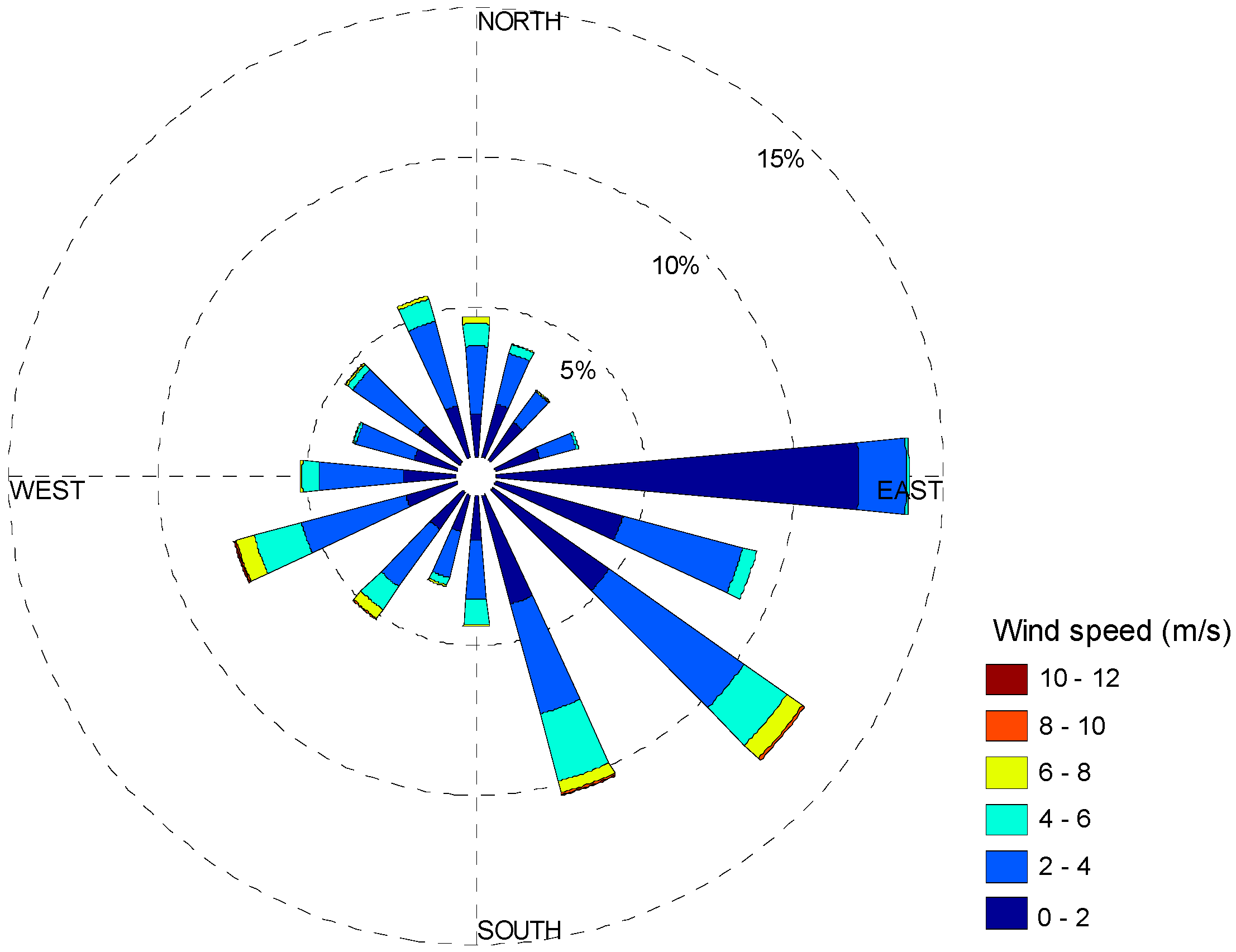
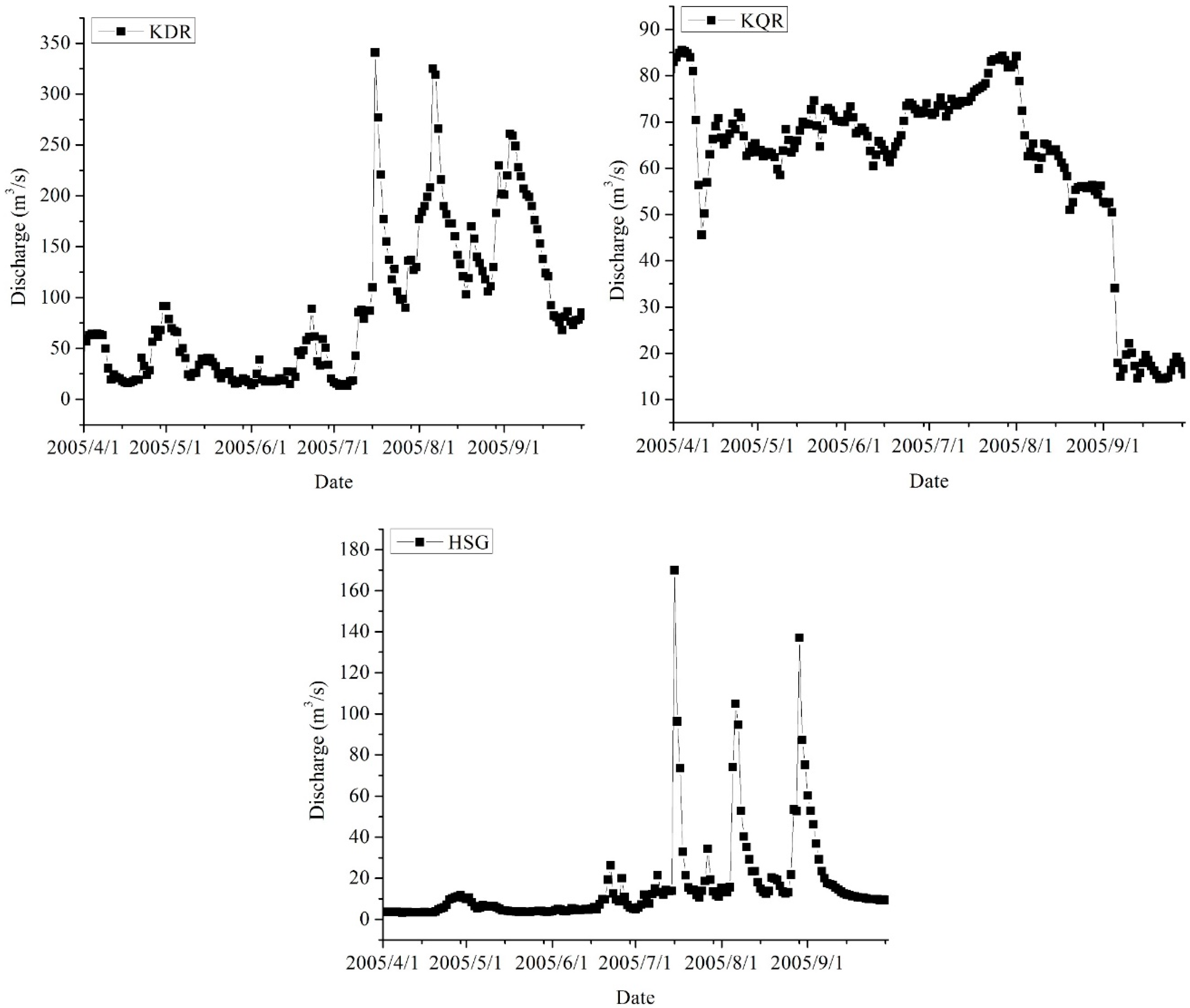
EFDC is forced by atmospheric conditions (e.g., wind shear, evaporation, and precipitation) and tributary inflow/outflows, among other factors. Hourly meteorological data of 2005 at Yanqi weather station (Figure 1) in the vicinity of Bosten Lake, including air temperature, wind speed and direction, atmospheric pressure, cloud cover, relative humidity, pan evaporation, and precipitation, were obtained from the China Meteorological Administration. The wind rose map of the station is presented in Figure 2. Due to the absence of solar radiation observations at Yanqi Station, or neighboring areas in 2005, solar radiation was calculated by the method of Rosati and Miyakoda (1988) [48] and presumed to be the same in the whole model area. The solar attenuation coefficient was set as 0.45. The model flow boundary conditions included two inflows from the main stream, the Kaidu River at the southwest and agriculture drainage at the Huangshuigou region at the northwest, and one outflow to the Kongque River at the southwest of the lake (Figure 1). Daily volumetric flow rate of river (Figure 3) and water temperature data specified for the inflow of the Kaidu River at Yanqi hydrological station and outflow of the Kongque River at Tashidian (TSD) hydrological station were acquired from the Hydrological Yearbook of the People’s Republic of China [49]. The time series of the Kaidu River discharge was taken as the inflow discharge into the Bosten Lake. In 2005, the Kaidu River discharges varied from 13.2 to 341 m3/s, having a mean of 67.1 m3/s. The time series of the Kongque River discharge was set as the outflow discharge out of the Bosten Lake. To simulate the real inflow and outflow of the lake, some factors were applied to the river inflow and outflow. Salinity of the inflows was set by the data obtained from interpolation of several monthly observations acquired at a nationally-managed environmental monitoring station.
The initial conditions involving water temperature and water salinity, and water level were set as constant values. The lake water surface was assumed to be horizontally flat. The initial water level was specified as 1047.5 m of the daily value of the Bohu hydrological station on 1 April 2005. The initial water flow rate was specified as zero.
Parameters associated with the Mellor–Yamada turbulence model [45] were specified as the suggested values that was used in the Princeton Ocean Model [50]. Similarly, the dimensionless horizontal viscosity in the Smagorinsky equation [51] was specified as a given value of 0.1 [52]. Bottom roughness (Z0) was specified as a representative value of 0.0036 m [42,50] for water level calibration. Critical wet and dry depth were specified as 0.1.
A two-time level explicit finite-difference scheme was used in the time integration of the model. Through an internal/external mode-splitting procedure, the internal shear (or baroclinic mode computed across each sigma layer) separated from the external free-surface gravity wave (or barotropic mode computed on the depth average). The model was executed using a 25 s time step to meet the needs of the stability criterion of Courant–Fredrichs–Lewy condition.
Model calibration and verification was dependent on water level data observed at Bohu hydrological station, as well as water temperature and salinity measures from 14 sites across the lake (Figure 1). The 2005 daily averaged water levels were obtained from hydrologic yearbooks of the People’s Republic of China. The water surface elevation varied substantially within a year, with the highest value of 1047.46 m during the winter, and the lowest value of 1046.87 m during the summer. The observations of lake spatial salinity and temperature were obtained from the Xinjiang Environmental Protection Academy of Science for 14 sites on 11 May, 10 June, 7 July, 5 August, and 3 September of 2005. Of these sites, sites 13 and 14 are situated near the Kaidu River, the freshwater region. The other sites are situated in oligosaline regions, where they are under the impact of human activities in terms of tourism or agriculture. Site 1 is situated to the southwest of the lake. Sites 7–12 are impacted by eutrophic and saline agriculture wastewater drainage from the western lakeshore and tourist sites on the western lakeside. Sites 5 and 4 are close to the tourist region of the northern lakeshore (Figure 1).
Because we are concerned with the impact of the hydraulic connectivity on the spatial-temporal salinity changes in Bosten Lake, three numerical experiments (Table 1) were carried out for studying the impacts of the hydrological connectivity scenarios on the salinity distribution of the lake. They were A2—the increasing of the inflow of the Kaidu River into the lake, A3—the transferring of some freshwater to the Huangshuigou region, and A4—the changing of the outflow positon from the outlet of the Kongque River to the Caohu region. The simulation A1 was driven by actual observed data and was subsequently considered as the control run. In simulation A1, the model was initialized using average water temperature and salinity on 5 April, and driven by hourly mean surface heat flux and wind stress, and daily average flows of the rivers. In total there were four simulations. Experiments A2–A4 were hydraulic connectivity scenarios. From simulations A1–A4, the influence of three connectivity scenarios on the salinity distribution of Bosten Lake can be found.
3. Results and Discussion
3.1. Model Validation
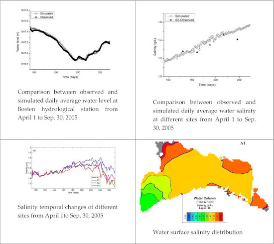
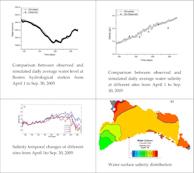
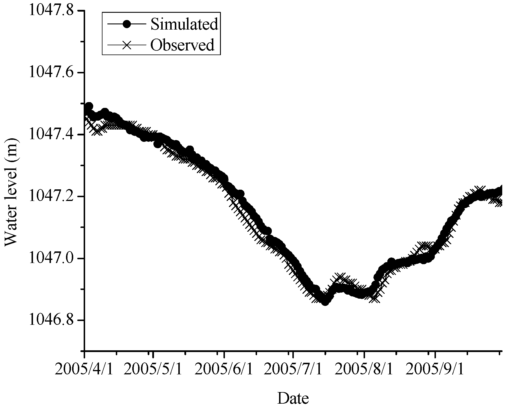
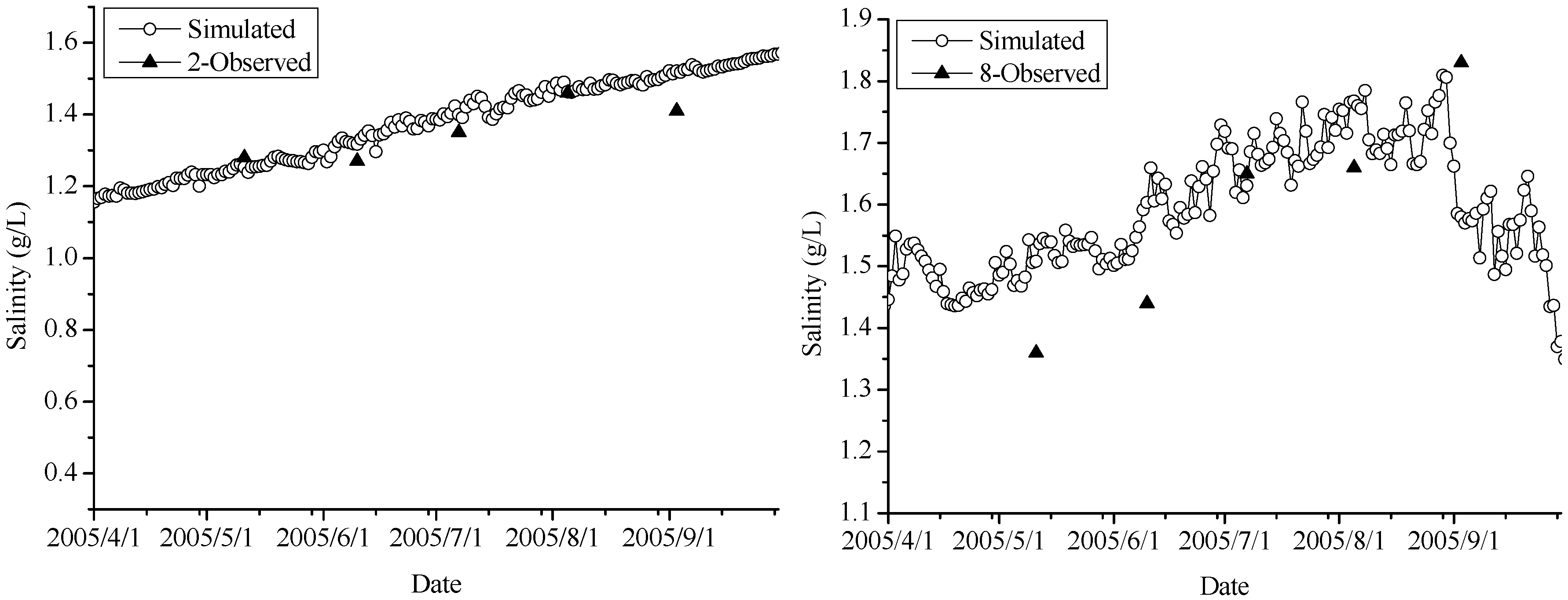
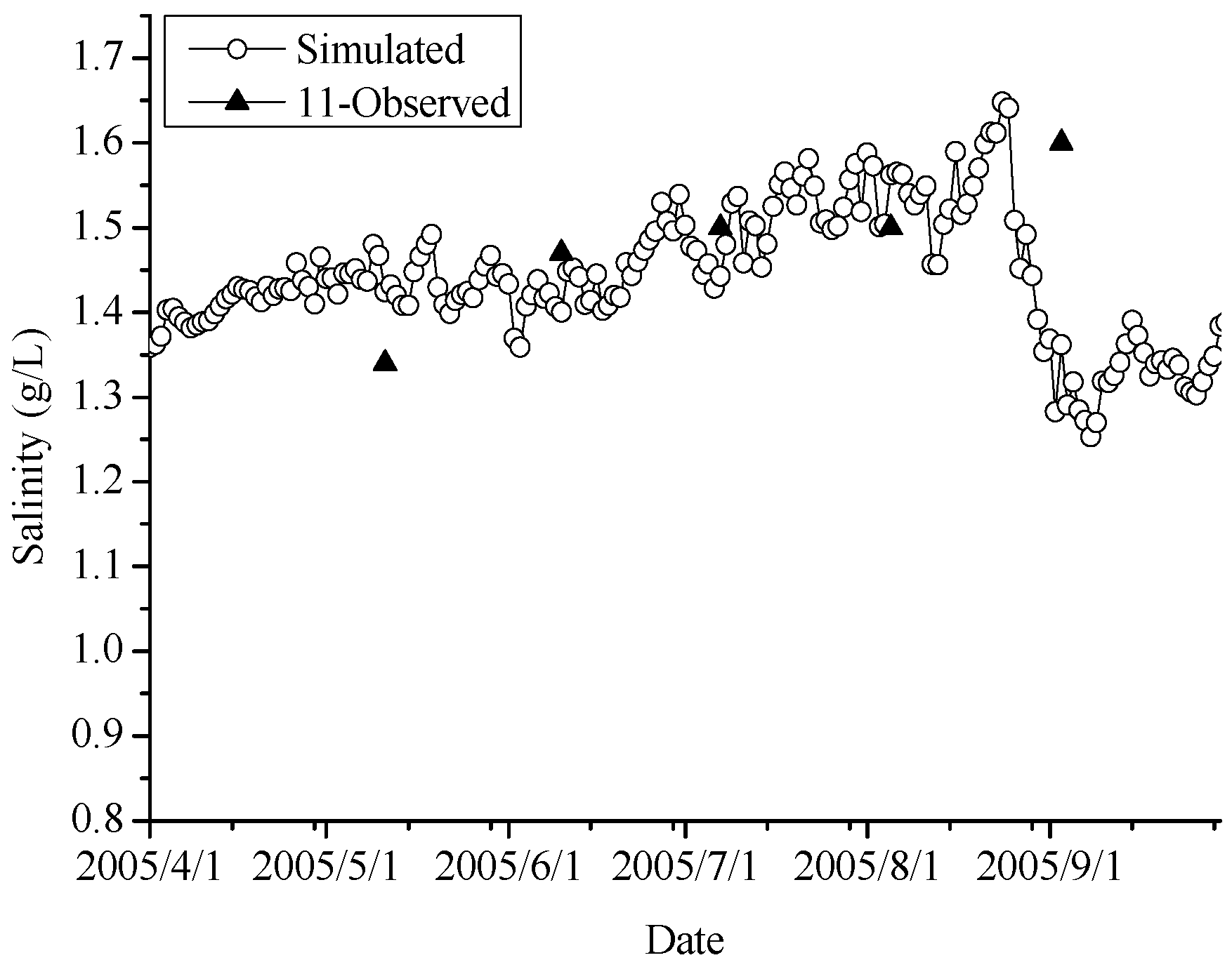
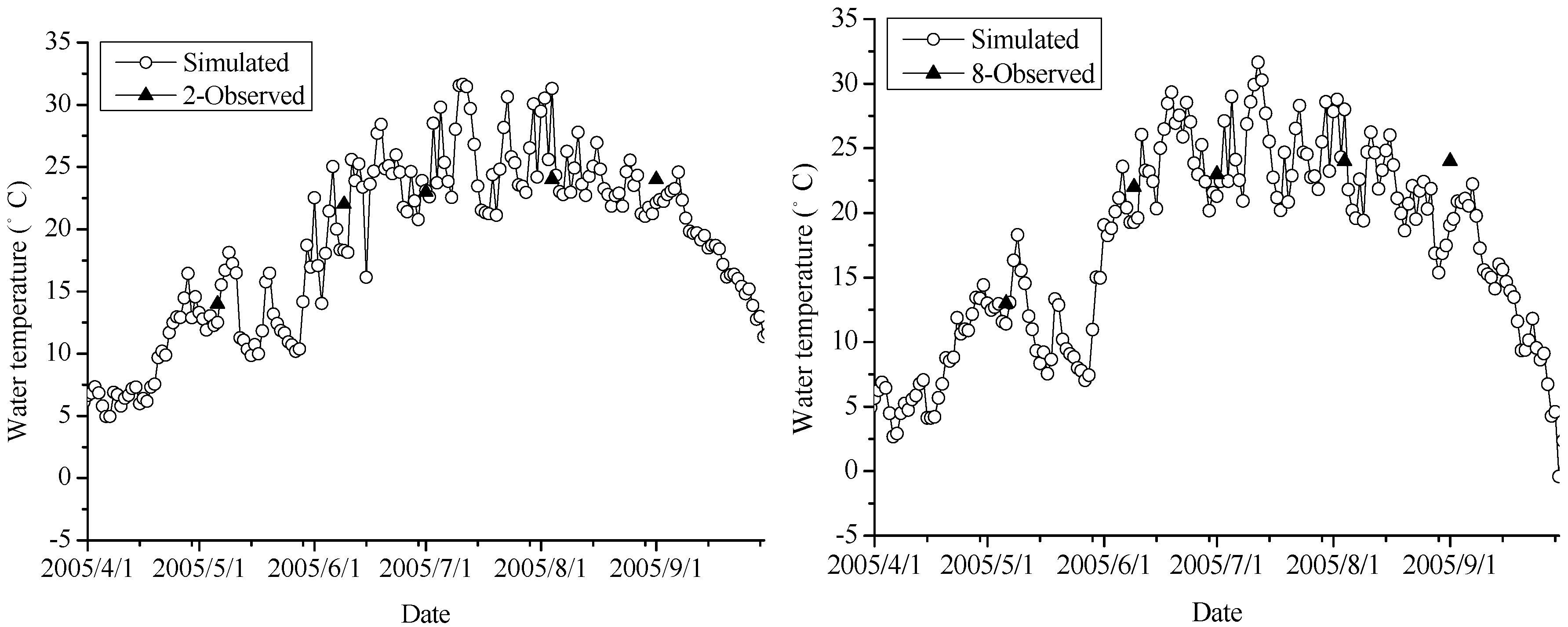
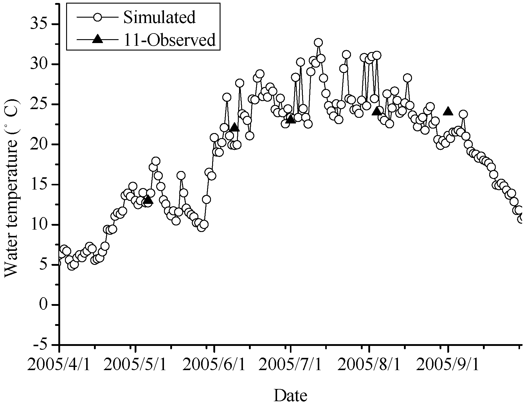
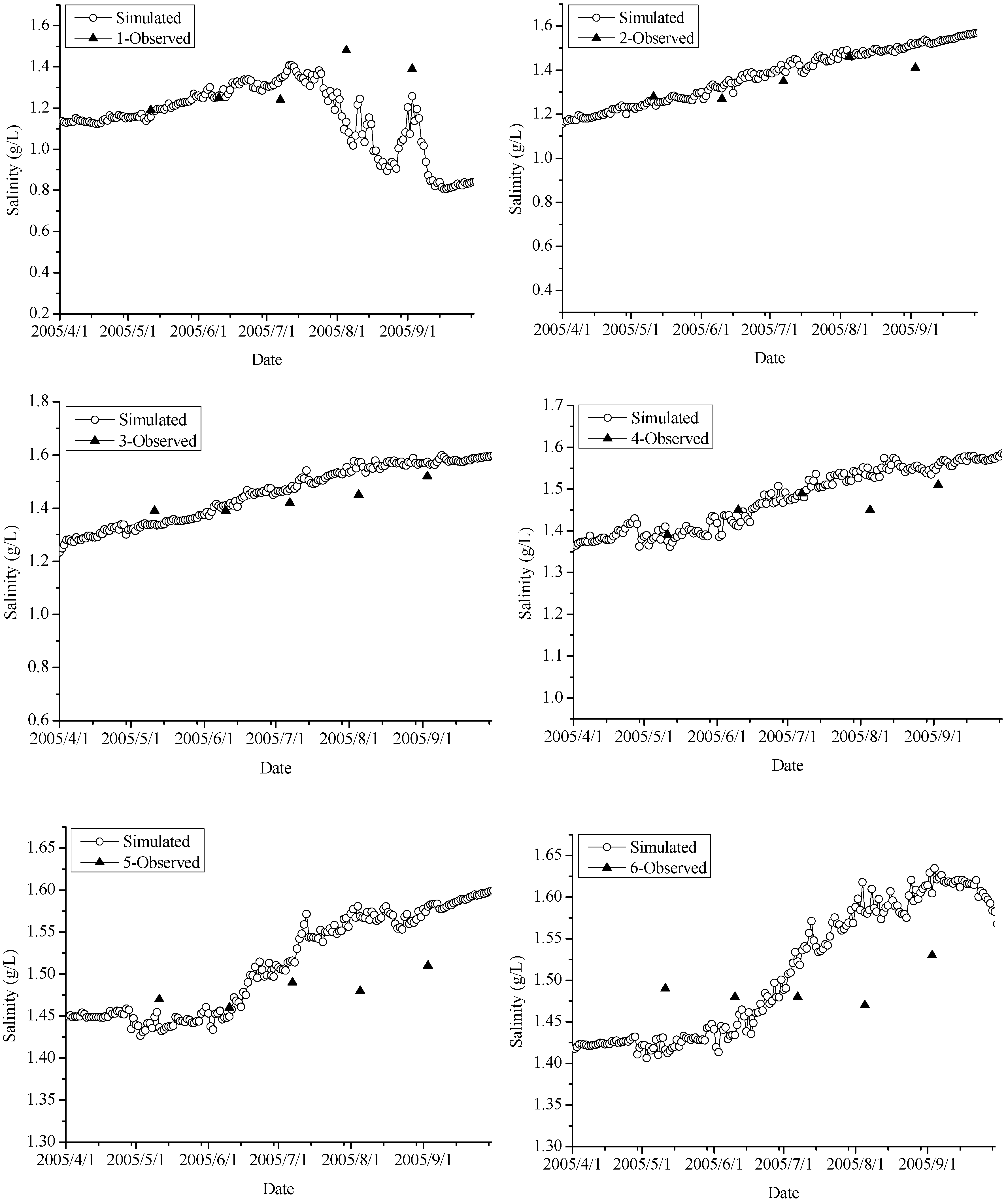
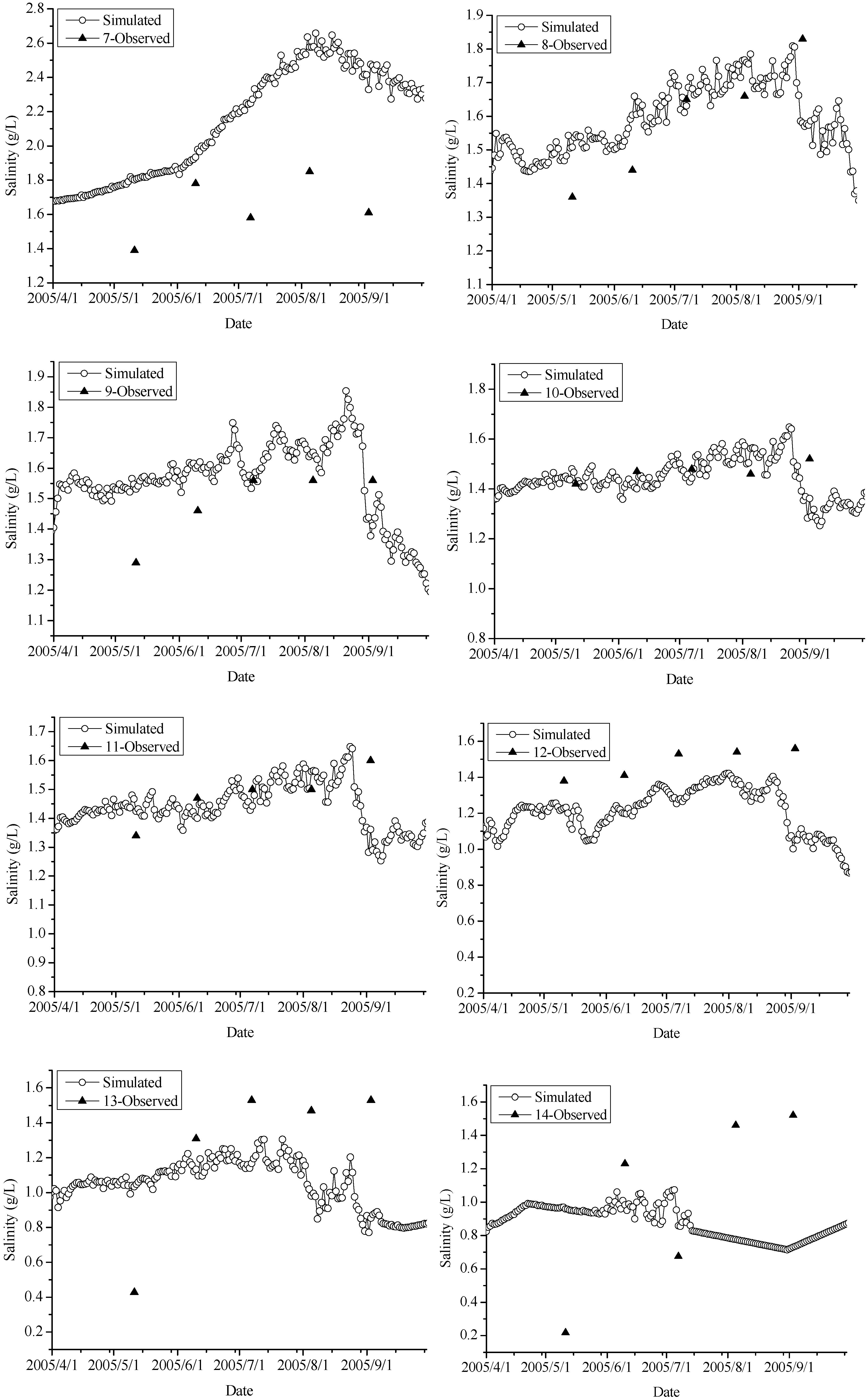
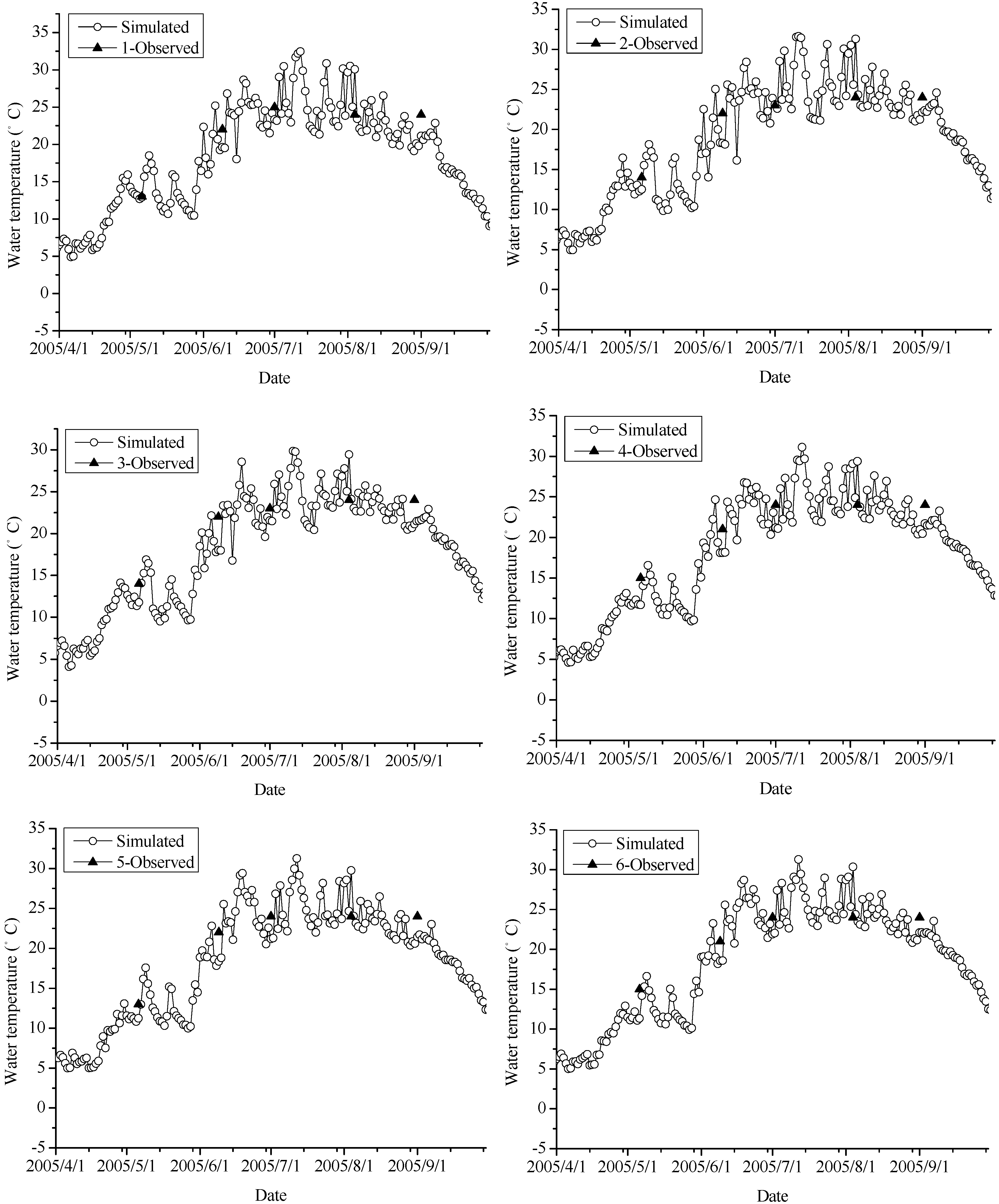
The model was calibrated by comparing the modelled results of water level, salinity, and temperature with the observed water level of Bosten hydrological station and salinity and temperature of different sites within the lake. Generally, the simulated values were in agreement with the observed data (Figure 4, Figure 5 and Figure 6). Here, we only showed the calibration results of S2, S8, and S11, as they were distributed in the typical places of the lake and can represent the whole lake condition (See the Appendix A for the calibration results of other sites). The modelled water level was almost equal to the observed data (Figure 4), which demonstrated that the model could model water surface variations considering changes in wind, freshwater discharge, evaporation, and precipitation. The water level of Bosten Lake presented a concave change during the simulation period, and was mainly influenced by the lake evaporation and the inflow and outflow discharges. However, the predicted salinity was slightly different from the observed data, which may have been due to the neglecting of the impact of the resuspended and dissolved bottom salt sediments. The predicted temperature was also a little higher than the observations, which may have been due to the neglecting of the spatial heterogeneity of the meteorological conditions, as well as the neglecting of the heat exchange between the bottom water and lakebed.
The root mean squared error (RMSE), mean absolute error (MAE), and mean absolute percentage error (MAPE) were applied to evaluate the average simulation error. The agreement between the simulated and measured water level at Bohu hydrological station (Figure 1) was reasonable, with an MAE value of 0.02 m, an RMSE value of 0.03 m, and an MAPE value of 0%, which meant the simulated and measured water levels were almost same (Figure 4, Table 2). The agreement between the measured and simulated water salinity at S2, S8, and S11 was satisfactory, with MAE values of 0.24, 0.17, and 0.19 g/L; RMSE values of 0.45, 0.19, and 0.31 g/L; and MAPE values of 16.24%, 10.36%, and 11.68%, respectively (Figure 5, Table 2). The agreement between the simulated and measured water temperature at S2, S8, and S11 was satisfactory, with MAE values of 3.53, 4.56, and 3.14 °C; RMSE values of 4.43, 5.86, and 4.08 °C; and MAPE values of 18.48%, 25.30%, and 15.94%, respectively (Figure 6, Table 2). The model has the possibility of simulating water level, temperature, and salinity with reasonable accuracy, which nonetheless needs to be improved. Overall, the model results are acceptable and can be used to analyze the salinity change due to different connectivity scenarios expressed by different inflows and outflows.
3.2. The Influences of Hydraulic Connectivity on Water Salinity
3.2.1. The Spatial Distribution of Water Salinity
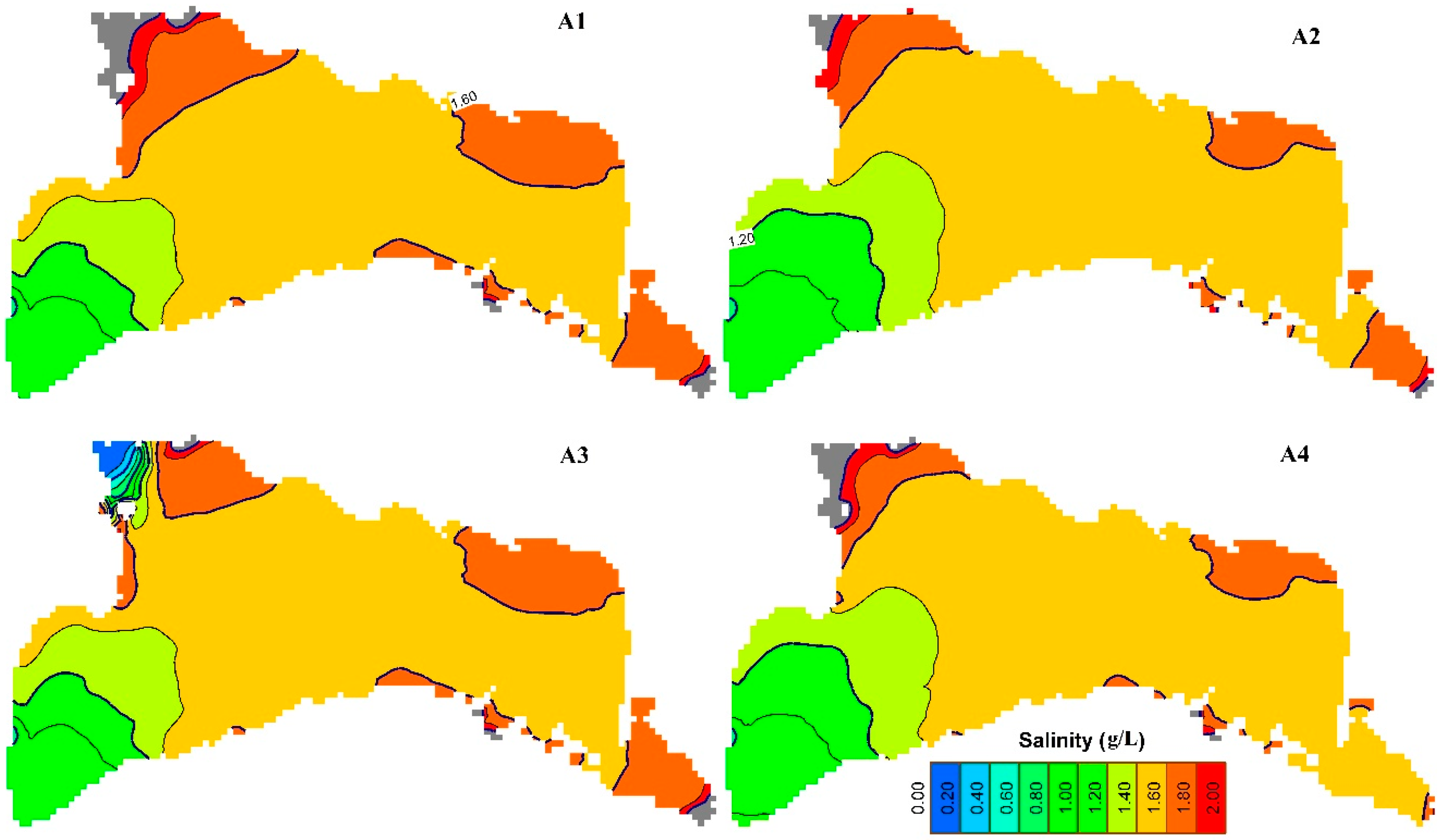
Through Figure 7 salinity distribution, we can see, compared to the validation value (A1), the increasing of the inflow quantity of the Kaidu River (A2), the transferring of freshwater to the Huangshuigou region (A3), and the changing of the outflow position from the outlet of the Kongque River to the Caohu region (A4) influenced the region more where the changes occurred. Under scenario A3, due to the limited quantity of the freshwater inflow, only the salinity of the Huangshuigou region deceased significantly, but that of the other regions changed little. In the scenarios A2 and A4, the high salinity region decreased and low salinity region increased in the lake. The increasing of the inflow of the Kaidu River and the change of the position of outflow to the Caohu region had similar impacts on lake salinity, except that the salinity of the region of Caohu decreased a large amount under A4. The increasing of the inflow of the Kaidu River mainly influenced the southeastern corner and east region of the lake. The changing of the outflow position to the Caohu region decreased the salinity of the Caohu region. Our simulation to some extent reflects other scholars’ results in that the freshwater inflows influenced the scope of the freshwater region in this lake [53], changing the salinity gradient of the lake [40].
3.2.2. The Temporal Changes of Water Salinity
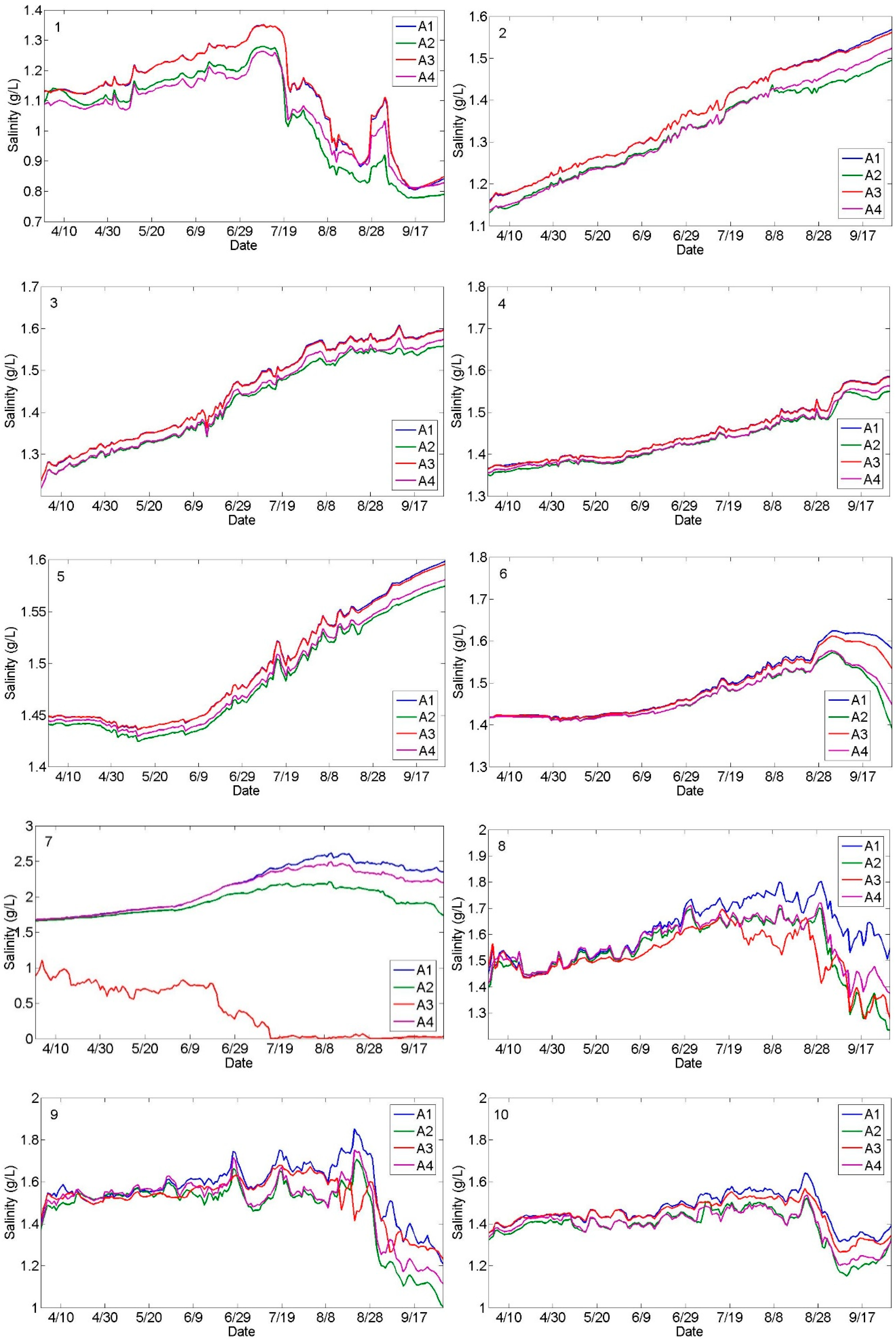
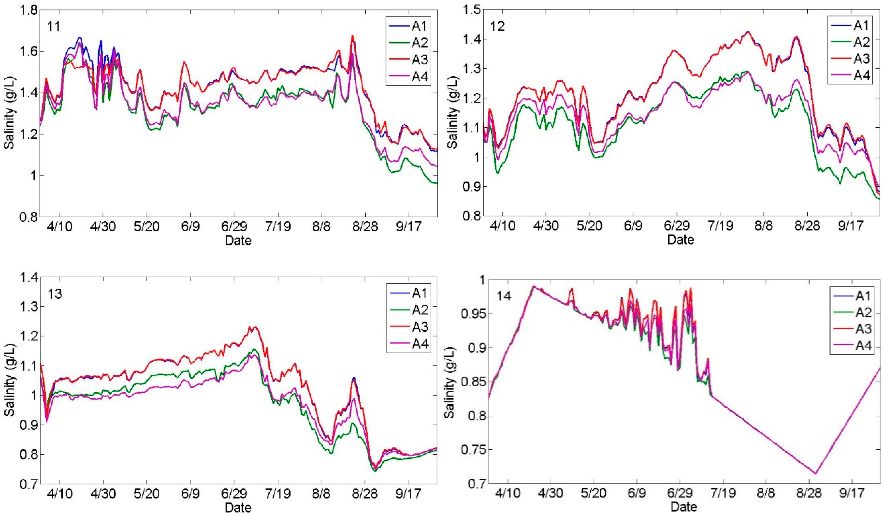
The salinity of the lake changed with time and place. At sites east of the lake, such as 1, 6, 7, 8, 9, 10, 11, 12, and 13, the salinity first increased and then decreased. In the sites in the center of the lake, such as 2, 3, 4, and 5, the salinity increased constantly during the study period. The time of reaching maximum salinity of the sites was different. At the region of the Kaidu River input, it appeared around July 9, such as at sites 1 and 13. At sites 2, 3, 4, and 5, it was around September 27. At the other sites, it was around August 28. From the salinity temporal changes of different sites (Figure 8), it can be seen that set conditions for scenario A3 only influenced the sites around the Huangshuigou Region—6, 7, 8, 9, and 10. The salinity time series of these sites under A3 were different from those under A1. The change of the outflow position from the Kongque River to the Caohu region and the increasing of the amount of the inflow of the Kaidu River decreased the salinity of different sites. At many sites, the change of the outflow position (A4) decreased the salinity similarly to the 50% increase of the inflow of the Kaidu River (A2). However, the A4 scenario did not need cost addition fresh water to decrease the lake salinity, and thus it is the optimum way to obtain/preserve freshwater lakes and save water resources in arid regions. In scenario A2, the 50% increase of the inflow of the Kaidu River decreased the salinity of different sites more than the other two scenarios because the discharge of the Kaidu River is freshwater and the inflow amount of water is high (annual value of 20.95 × 10⁸ m3).
3.2.3. The Amount of the Water Salinity Change under Different Scenarios
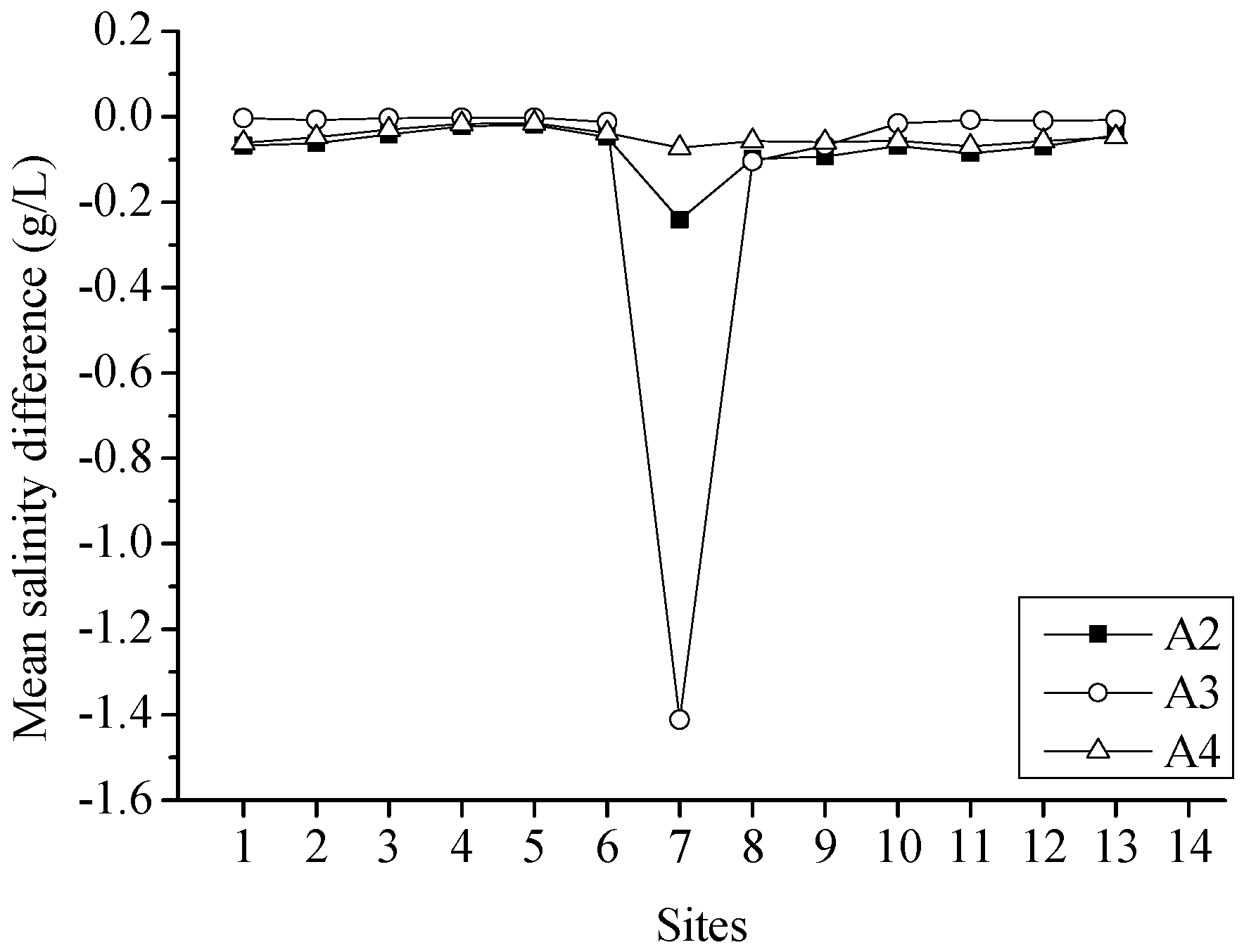
For quantifying the change of water salinity due to different scenarios, the mean difference of salinity between the scenario and the validation simulation over the study period was calculated with the following equation:
where represents different scenarios, is the validation simulation, and I is scenario. I = 1, 2, 3 represents A2, A3, and A4, respectively. J is time (days).
The A3 scenario was mainly influenced the Huangshuigou region. In the transferring of fresh water to the Huangshuigou region, the salinity of site 7 decreased extremely for around 1.4 g L−1 (68%) (Figure 9, Table 3). At sites 8 and 9, the salinity decreased around 0.1 g L−1. At sites 2, 6, 10, 11, 12, and 13 the salinity decreased around 0.01 g L−1. At sites 1, 3, 4, and 5, the salinity only decreased around 0.003 g L−1. The A2 and A4 scenarios influenced the east part sites and not the center sites. At sites 3, 4, and 5 under A2 and A4, the salinity decreased only 0.02 g L−1. At sites 1, 2, 8, 9, 10, 11, and 12, under A2 and A4, the salinity decreased around 0.1 g L−1. At sites 6 and 13, the salinity decreased around 0.04 g L−1. At site 7 under A2 and A4, the salinity decreased 0.24 and 0.07 g L−1 (Figure 9). The higher the salinity of the region, the more obvious it changed. For the lower salinity region, the changes in salinity were not obvious.
4. Conclusions
The hydraulic connectivity influences on water salinity of Bosten Lake were studied in terms of controlling the water salinization of Bosten Lake, providing information for hydraulic engineering control activities. This research obtained the spatial information of salinity in different situations, instead of a single value, for one whole spatial heterogeneous lake. Its findings can be used so that decision-makers can make more targeted decisions regarding different regions of a big lake, especially for those in a water shortage area.
A 50% increase of the quantity of the inflow from the Kaidu River, the transferring of freshwater to the Huangshuigou region of the lake, and the changing of the outflow position from the outlet of the Kongque River to the Caohu region, all decreased the salinity of the lake. The different hydraulic connectivity scenarios had different impacts in different regions of the lake. The transferring of 1 million cubic meters of freshwater to the Huangshuigou region mainly influenced the Huangshuigou region of the lake, which is useful mainly for the decrease of salinity in the northwestern region of the lake but not for the entire lake. If we want to control the lake salinity, adjusting hydraulic connectivity through changing the amount and position of the inflow and outflow of the lake is an alternative. A combination of all the three scenarios could be the best way to optimally decrease the salinity of Bosten Lake.
Author Contributions
Y.L. constructed the Bosten Lake EFDC model and wrote the first draft. A.B. was in charge of this work. All authors have read and agreed to the published version of the manuscript.
Funding
This study was funded by the National Key Research and Development Program of China, grant number 2017YFC0404501; the Strategic Priority Research Program of Chinese Academy of Sciences, grant number XDA20060303; Tianshan Innovation Team Project of Xinjiang Department of Science and Technology, grant number Y744261; National Natural Science Foundation of China (NSFC), grant number 41101040; and “Western Light” Talents Training Program of Chinese Academy of science (CAS), grant number XBBS201005.
Acknowledgments
We are extremely grateful to the editors Cici Hu, Evelyn Ning, and Cora Zheng and two anonymous reviewers for providing many important suggestions that were very helpful in the improvement of this paper.
Conflicts of Interest
All authors state no conflicts of interest.
Appendix A. The Calibration Results of Sites 1-14 and Hydrodynamic Model Equations Are as Follows
Figure A1.
Comparison between observed and simulated daily average water salinity at sites 1-14 from 1 April to 30 September 2005.
Figure A1.
Comparison between observed and simulated daily average water salinity at sites 1-14 from 1 April to 30 September 2005.


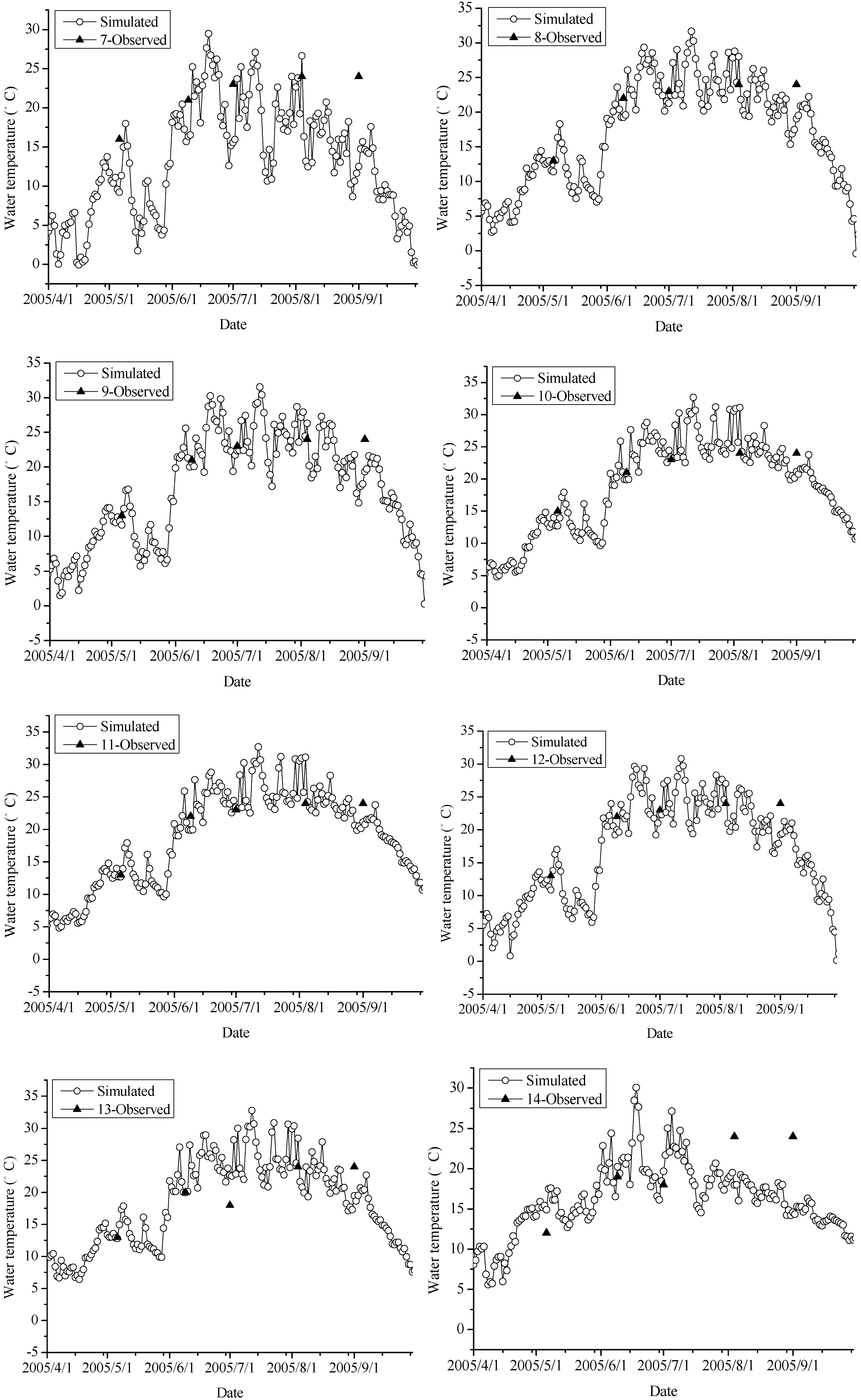
Figure A2.
Comparison between observed and simulated daily average water temperature at sites 1-14 from 1 April to 30 September 2005.
Figure A2.
Comparison between observed and simulated daily average water temperature at sites 1-14 from 1 April to 30 September 2005.


Table A1.
Statistics on water salinity at sites 1-14: observation against simulation.
| Sites | Mean Simulated (g/L) | Mean Observed (g/L) | MAE (g/L) | MAPE | RMSE (g/L) |
|---|---|---|---|---|---|
| 1 | 1.07 | 1.35 | 0.31 | 20.99 | 0.49 |
| 2 | 1.28 | 1.38 | 0.24 | 16.24 | 0.45 |
| 3 | 1.44 | 1.45 | 0.13 | 9.02 | 0.20 |
| 4 | 1.47 | 1.47 | 0.08 | 5.05 | 0.10 |
| 5 | 1.50 | 1.51 | 0.10 | 6.21 | 0.14 |
| 6 | 1.48 | 1.51 | 0.10 | 6.20 | 0.13 |
| 7 | 2.08 | 1.69 | 0.58 | 34.26 | 0.61 |
| 8 | 1.55 | 1.60 | 0.17 | 10.36 | 0.19 |
| 9 | 1.48 | 1.52 | 0.18 | 12.28 | 0.22 |
| 10 | 1.38 | 1.54 | 0.20 | 12.04 | 0.31 |
| 11 | 1.38 | 1.51 | 0.19 | 11.68 | 0.31 |
| 12 | 1.07 | 1.41 | 0.34 | 25.17 | 0.38 |
| 13 | 0.91 | 1.15 | 0.42 | 46.98 | 0.45 |
| 14 | 0.78 | 1.00 | 0.48 | 79.61 | 0.55 |
Table A2.
Statistics on water temperature at sites 1-14: observation against simulation.
| Sites | Mean Simulated (℃) | Mean Observed (℃) | MAE (℃) | MAPE | RMSE (℃) |
|---|---|---|---|---|---|
| 1 | 18.97 | 20.50 | 3.55 | 18.41 | 4.51 |
| 2 | 19.27 | 20.33 | 3.53 | 18.48 | 4.43 |
| 3 | 18.53 | 20.33 | 3.61 | 18.82 | 3.94 |
| 4 | 18.59 | 20.50 | 3.71 | 19.44 | 3.92 |
| 5 | 18.53 | 19.80 | 3.19 | 16.38 | 3.43 |
| 6 | 18.77 | 20.50 | 3.84 | 20.53 | 4.31 |
| 7 | 13.52 | 20.50 | 7.86 | 41.70 | 8.78 |
| 8 | 16.94 | 20.17 | 4.56 | 25.30 | 5.86 |
| 9 | 17.30 | 20.00 | 3.46 | 20.02 | 5.16 |
| 10 | 19.51 | 20.33 | 3.31 | 17.39 | 4.12 |
| 11 | 19.51 | 20.17 | 3.14 | 15.94 | 4.08 |
| 12 | 17.10 | 20.17 | 4.08 | 23.30 | 5.47 |
| 13 | 18.17 | 19.00 | 3.87 | 21.20 | 4.99 |
| 14 | 15.50 | 18.67 | 5.09 | 27.69 | 6.11 |
Table A3.
Statistics on water level at Bohu hydrological station (BH): observation against simulation.
Table A3.
Statistics on water level at Bohu hydrological station (BH): observation against simulation.
| Hydrological Station | Mean Simulated (m) | Mean Observed (m) | MAE (m) | MAPE | RMSE (m) |
|---|---|---|---|---|---|
| BH | 1047.15 | 1047.14 | 0.02 | 0.00 | 0.03 |
The EFDC hydrodynamic model includes equations of continuity, momentum, state and transport for salinity and temperature shown below.
where, u and v are the horizontal velocity components in the curvilinear, orthogonal coordinates x and y (m/s); z is the sigma coordinate (dimensionless); t is time (s); , are the square roots of the diagonal components of the metric tensor (m); m = is the Jacobian or square root of the metric tensor determinant; is the vertical velocity component in sigma coordinate (m/s), and is the physical vertical velocity (m/s); , is the total water depth; h is the water depth bellow the vertical reference level (m); ζ is the water surface elevation above the vertical reference level (m); is the Coriolis coefficient (1/s); is the horizontal momentum and mass diffusivity (m2/s); is the vertical turbulent or eddy viscosity coefficient (m2/s); is the vertical turbulent diffusivity (m2/s); is the vegetation resistance coefficient (dimensionless); is the dimensionless projected vegetation area normal to the flow per unit horizontal area (dimensionless); is the source/sink terms for the mass conservation equation (m³/s); and are the source/sink terms for the horizontal momentum in the x and y directions, respectively (m2/s2); and are the horizontal diffusion and thermal sources and sinks; is the disturbance density, generally a function of temperature and salinity; is the reference water density (kg/m³); p is the physical pressure in excess of the reference density hydrostatic pressure (m2/s2); is the barotropic pressure (Pa); b is buoyancy; T is the water temperature (°C); S is the water salinity (g/L).
References
- Hammer, U.T. Saline Lake Ecosystem of the World; Springer Science & Business Media: Berlin/Heidelberg, Germany, 1986. [Google Scholar]
- Lioubimtseva, E.; Henebry, G.M. Climate and environmental change in arid Central Asia: Impacts, vulnerability, and adaptations. J. Arid Environ. 2009, 73, 963–977. [Google Scholar] [CrossRef]
- Gross, M. The world’s vanishing lakes. Curr. Biol. 2017, 27, R43–R46. [Google Scholar] [CrossRef]
- Wurtsbaugh, W.A.; Miller, C.; Null, S.E.; DeRose, R.J.; Wilcock, P.; Hahnenberger, M. Decline of the world’s saline lakes. Nat. Geosci. 2017, 10, 816–821. [Google Scholar] [CrossRef]
- Schofield, N.J.; Ruprecht, J.K. Regional analysis of stream salinisation in southwest Western Australia. J. Hydrogeol. 1989, 112, 19–39. [Google Scholar] [CrossRef]
- Zuo, Q.T.; Dou, M.; Chen, X.; Zhou, K.F. Physically-based model for studying the salinization of Bosten Lake in China. Hydrol. Sci. J. 2006, 51, 432–449. [Google Scholar] [CrossRef] [Green Version]
- Dai, J.Y.; Tang, X.M.; Gao, G.; Chen, D.; Shao, K.Q.; Cai, X.L.; Zhang, L. Effects of salinity and nutrients on sedimentary bacterial communities in oligosaline Lake Bosten, northwestern China. Aquat. Microb. Ecol. 2013, 69, 123–134. [Google Scholar] [CrossRef]
- Williams, W.D. Anthropogenic salinisation of inland waters. Hydrobiologia 2001, 466, 329–337. [Google Scholar] [CrossRef]
- Vitousek, P.M.; Mooney, H.A.; Lubchenco, J.; Melillo, J.M. Human domination of Earth’s ecosystems. Science 1997, 277, 494–499. [Google Scholar] [CrossRef] [Green Version]
- Yechieli, Y.; Wood, W.W. Hydrogeologic processes in saline systems: Playas, sabkhas, and saline lakes. Earth Sci. Rev. 2002, 58, 343–365. [Google Scholar] [CrossRef]
- Lerman, A. Saline Lakes’ response to global change. Aquat. Geochem. 2009, 15, 1–5. [Google Scholar] [CrossRef]
- Crosbie, R.S.; McEwan, K.L.; Jolly, I.D.; Holland, K.L.; Lamontagne, S.; Moe, K.G.; Simmons, C.T. Salinization risk in semi-arid floodplain wetlands subjected to engineered wetting and drying cycles. Hydrol. Process. 2009, 23, 3440–3452. [Google Scholar] [CrossRef]
- Feng, Q.; Cheng, G.D. Current situation, problems and rational utilization of water resources in arid northwestern China. J. Arid Environ. 1998, 40, 373–382. [Google Scholar]
- Williams, W.D. Salinisation: A major threat to water resources in the arid and semi-arid regions of the world. Lakes Reserv. Res. Manag. 1999, 4, 85–91. [Google Scholar] [CrossRef]
- Alcocer, J.; Escobar, E.; Lugo, A. Water use (and abuse) and its effects on the crater-lakes of Valle de Santiago, Mexico. Lakes Reserv. Res. Manag. 2000, 5, 145–149. [Google Scholar] [CrossRef]
- Migahid, M.M. Effect of salinity shock on some desert species native to the northern part of Egypt. J. Arid Environ. 2003, 53, 155–167. [Google Scholar] [CrossRef]
- Huang, X.; Chen, F.; Fan, Y.; Yang, M. Dry late-glacial and early Holocene climate in arid central Asia indicated by lithological and palynological evidence from Bosten Lake, China. Quat. Int. 2009, 194, 19–27. [Google Scholar] [CrossRef]
- Liu, W.C.; Hsu, M.H.; Kuo, A.Y.; Hung, H.Y. Effect of channel connection on flow and salinity distribution of Danshuei River estuary. Appl. Math. Model. 2007, 31, 1015–1028. [Google Scholar] [CrossRef]
- Li, Y.; Zhang, Q.; Cai, Y.; Tan, Z.; Wu, H.; Liu, X.; Yao, J. Hydrodynamic investigation of surface hydrological connectivity and its effects on the water quality of seasonal lakes: Insights from a complex floodplain setting (Poyang Lake, China). Sci. Total Environ. 2019, 660, 245–259. [Google Scholar] [CrossRef]
- Wolf, K.L.; Noe, G.B.; Ahn, C. Hydrologic connectivity to streams increases nitrogen and phosphorus inputs and cycling in soils of created and natural floodplain wetlands. J. Environ. Qual. 2013, 42, 1245–1255. [Google Scholar] [CrossRef] [Green Version]
- Yu, X.; Hawley-Howard, J.; Pitt, A.L.; Wang, J.J.; Baldwin, R.F.; Chow, A.T. Water quality of small seasonal wetlands in the Piedmont ecoregion, South Carolina, USA: Effects of land use and hydrological connectivity. Water Res. 2015, 73, 98–108. [Google Scholar] [CrossRef]
- Lew, S.; Glińska-Lewczuk, K.; Burandt, P.; Obolewski, K.; Goździejewska, A.; Lew, M.; Dunalska, J. Impact of environmental factors on bacterial communities in floodplain lakes differed by hydrological connectivity. Limnol.-Ecol. Manag. Inland Waters 2016, 58, 20–29. [Google Scholar] [CrossRef]
- Kang, L.; Guo, X.M. Hydrodynamic effects of reconnecting lake groups with Yangtze River in China. Water Sci. Eng. 2011, 4, 405–420. [Google Scholar]
- Obolewski, K.; Strzelczak, A.; Glińska-Lewczuk, K. Does hydrological connectivity affect the composition of macroinvertebrates on Stratiotes aloides L. in oxbow lakes? Ecol. Eng. 2014, 66, 72–81. [Google Scholar] [CrossRef]
- Xia, S.X.; Liu, Y.; Wang, Y.Y.; Chen, B.; Jia, Y.F.; Liu, G.H.; Yu, X.B.; Wen, L. Wintering waterbirds in a large river floodplain: Hydrological connectivity is the key for reconciling development and conservation. Sci. Total Environ. 2016, 573, 645–660. [Google Scholar] [CrossRef] [PubMed]
- Merel, V.D.M.; Hudson, P.F. The influence of floodplain geomorphology and hydrologic connectivity on alligator gar (Atractosteus spatula) habitat along the embanked floodplain of the Lower Mississippi River. Geomorphology 2018, 302, 62–75. [Google Scholar]
- Zuecco, G.; Rinderer, M.; Penna, D.; Borga, M.; Van, M.H.J. Quantification of subsurface hydrologic connectivity in four headwater catchments using graph theory. Sci. Total Environ. 2019, 646, 1265–1280. [Google Scholar] [CrossRef]
- Zhou, L.; Zhou, Y.; Hu, Y.; Cai, J.; Bai, C.; Shao, K.; Gao, G.; Zhang, Y.; Jeppesen, E.; Tang, X. Hydraulic connectivity and evaporation control the water quality and sources of chromophoric dissolved organic matter in Lake Bosten in arid northwest China. Chemosphere 2017, 188, 608–617. [Google Scholar] [CrossRef]
- Liu, Y.; Bao, A.M.; Chen, X.; Zhong, R.S. A Model Study of the Discharges Effects of Kaidu River on the Salinity Structure of Bosten Lake. Water 2019, 11, 8. [Google Scholar] [CrossRef] [Green Version]
- Xie, G.J.; Zhang, J.; Tang, X.M.; Cai, Y.; Gao, G. Spatio-temporal heterogeneity of water quality and succession patterns in Lake Bosten during the past 50 years. J. Lake Sci. 2011, 23, 988–998. [Google Scholar]
- Cheng, Q.C. Studies on Bosten Lake; Hehai Unversity Press: Nanjing, China, 1995. [Google Scholar]
- Wei, K.Y.; Lee, M.Y.; Wang, C.H.; Wang, Y.; Lee, T.Q.; Yao, P. Stable isotopic variations in oxygen and hydrogen of waters in Lake Bosten region, Southern Xinjiang, Western China. West. Pac. Earth Sci. 2002, 2, 67–82. [Google Scholar]
- Li, Y.A.; Tan, Y.; Jiang, F.Q.; Wang, Y.J.; Hu, R.J. Study on hydrological features of the Kaidu River and the Bosten Lake in the second half of 20th century. J. Glaciol. Geocryol. 2003, 25, 215–218. [Google Scholar]
- Xu, H.L.; Guo, Y.P.; Li, W.H. Analysis on the water pollution in Bosten Lake, Xinjiang. Arid Zone Res. 2003, 20, 192–196. [Google Scholar]
- Xia, J.; Zuo, Q.T.; Shao, M.C. Sustainable Management of Water Resources in Lake Bosten; Chinese Science Press: Beijing, China, 2003. [Google Scholar]
- Zuo, Q.T.; Chen, X. Water Planning and Management Meeting Sustainable Development; China Hydropower Press: Beijing, China, 2003. [Google Scholar]
- Cheng, Z.C.; Li, Y.A. Water-salt equilibrium and mineralization of Bosten Lake, Xinjiang. Arid Land Geogr. 1997, 20, 43–49. [Google Scholar]
- Zhao, J.F.; Qin, D.H.; Nagashima, H.; Lei, J.Q.; Wei, W.S. Analysis of mechanism of the salinization process and the salinity variation in Bosten Lake. Adv. Water Sci. 2007, 18, 475–482. [Google Scholar]
- Guo, M.J.; Wu, W.; Zhou, X.D.; Chen, Y.M.; Li, J. Investigation of the dramatic changes in lake level of the Bosten Lake in northwestern China. Theor. Appl. Climatol. 2015, 119, 341–351. [Google Scholar] [CrossRef]
- Tang, X.M.; Xie, G.J.; Shao, K.Q.; Bayartu, S.; Chen, Y.G.; Gao, G. Influence of salinity on the bacterial community composition in Lake Bosten, a large oligosaline lake in arid northwestern China. Appl. Environ. Microb. 2012, 78, 4748–4751. [Google Scholar] [CrossRef] [Green Version]
- Sai, B.; Huang, J.; Xie, G.; Feng, L.; Hu, S.; Tang, X. Response of planktonic bacterial abundance to eutrophication and salinization in Lake Bosten, Xinjiang. J. Lake Sci. 2011, 23, 934–941. (In Chinese) [Google Scholar]
- Hamrick, J.M. A Three-dimensional Environmental Fluid Dynamics Computer Code: Theoretical and Computational Aspects. The College of William and Mary, Virginia Institute of Marine Science. Spec. Rep. 1992, 317, 63. [Google Scholar]
- Hamrick, J.M. In: Tetra Tech, I. The Environmental Fluid Dynamics Code: Theory and Computation; US EPA: Fairfax, VA, USA, 2007.
- Hamrick, J.M. In: Tetra Tech, I. The Environmental Fluid Dynamics Code: User Manual; US EPA: Fairfax, VA, USA, 2007.
- Mellor, G.L.; Yamada, T. Development of a turbulence closure model for geophysical fluid problems. Rev. Geophys. Space Phys. 1982, 20, 851–875. [Google Scholar] [CrossRef] [Green Version]
- Hamrick, J.M.; Wu, T.S. Computational design and optimization of the EFDC/ HEM3D surface water hydrodynamic and eutrophication models. In Next Generation Environmental Models and Computational Methods; Delich, G., Wheeler, M.F., Eds.; Society of Industrial and Applied Mathematics: Philadelphia, PA, USA, 1997; pp. 143–156. [Google Scholar]
- Galperin, B.; Kantha, L.H.; Hassid, S.; Rosati, A. A quasi-equilibrium turbulent energy model for geophysical flows. J. Atmos. Sci. 1988, 45, 55–62. [Google Scholar] [CrossRef] [Green Version]
- Rosati, A.; Miyakoda, K. A general circulation model for upper ocean simulation. J. Phys. Oceanogr. 1988, 18, 1601–1626. [Google Scholar] [CrossRef]
- SLB. Hydrological Yearbook of the People’s Republic of China of Inland Rivers and Lakes in the Southern Tian-Shan Mountains; SLB: Xinjiang, China; Beijing, China, 2005. [Google Scholar]
- HydroQual Inc. A Primer for ECOMSED, Version 1.3, User’s Manual; HydroQual Inc., 1 Lethbridge Plaza: Mahwah, NJ, USA, 2002; p. 188. [Google Scholar]
- Smagorinsky, J. General Circulation Experiments with the Primitive Equations, I. The Basic Experiment. Mon. Weather Rev. 1963, 91, 99–164. [Google Scholar] [CrossRef]
- Berntsen, J. Internal pressure errors in sigma-coordinate ocean models. J. Atmos. Oceanic. Technol. 2002, 19, 1403–1414. [Google Scholar] [CrossRef]
- Xiao, M.; Wu, F.; Liao, H.; Li, W.; Lee, X.; Huang, R. Characteristics and distribution of low molecular weight organic acids in the sediment porewaters in Bosten Lake, China. J. Environ. Sci. 2010, 22, 328–337. [Google Scholar] [CrossRef]
Figure 1.
The schematic map of Bosten Lake (in which black sold circles represent the observed sites; KDR, KQR, HSG, CH, YQ, and BH stand for the Kaidu River, the Kongque River, the Huangshuigou region, the Caohu region, and Yanqi and Bohu stations, respectively; the black stars represent the inlets of KDR and HSG, the outlets of KQR and CH; the black arrows show the schematic flow direction of the inlet and outlet; the bathymetry was described by Kriging interpolation used for EFDC (Environmental Fluid Dynamics Code) modeling).

Figure 2.
Wind rose map at the Yanqi station during the simulation period.

Figure 3.
The flow rate of hydrological stations of the Kaidu River (KDR), the Huangshuigou region (HSG), and the Kongque River (KQR) taken from the Hydrological Yearbook [48] was applied in forcing the Bosten Lake model during simulation period from 00:00 1 April to 00:00 30 September 2005.
Figure 3.
The flow rate of hydrological stations of the Kaidu River (KDR), the Huangshuigou region (HSG), and the Kongque River (KQR) taken from the Hydrological Yearbook [48] was applied in forcing the Bosten Lake model during simulation period from 00:00 1 April to 00:00 30 September 2005.

Figure 4.
Comparison between observed and simulated daily average water level at Bosten hydrological station from 1 April 2005 to 30 September 2005.
Figure 4.
Comparison between observed and simulated daily average water level at Bosten hydrological station from 1 April 2005 to 30 September 2005.

Figure 5.
Comparison between observed and simulated daily average water salinity at sites 2, 8, and 11 from 1 April 2005 to 30 September 2005.
Figure 5.
Comparison between observed and simulated daily average water salinity at sites 2, 8, and 11 from 1 April 2005 to 30 September 2005.


Figure 6.
Comparison between observed and simulated daily average water temperature at sites 2, 8, and 11 from 1 April 2005 to 30 September 2005.
Figure 6.
Comparison between observed and simulated daily average water temperature at sites 2, 8, and 11 from 1 April 2005 to 30 September 2005.


Figure 7.
Water surface salinity distribution on 15 August 2005 under different simulations: (A1) real condition, (A2) KDR inflow increase by 50%, (A3) 1 × 10⁸ m3/a freshwater transfer into HSG, and (A4) change of the outflow from KQR to CH (in which KDR, KQR, HSG, and CH stand for the Kaidu River, the Kongque River, the Huangshuigou region, and the Caohu region, respectively).

Figure 8.
Salinity temporal changes at sites 1–14 from 1 April 2005 to 30 September 2005 (in which simulations are A1—real condition, A2—KDR inflow increase by 50%, A3—1 × 10⁸ m3/a freshwater transfer into HSG, and A4—change of the outflow from KQR to CH; KDR, KQR, HSG, and CH stand for the Kaidu River, the Kongque River, the Huangshuigou region, and the Caohu region, respectively).


Figure 9.
The mean difference of salinity between the scenario and the validation simulation at sites 1-14 (A1—real condition) over the study period (in which simulations are A2—KDR inflow increase by 50%, A3—1 × 10⁸ m3/a freshwater transfer into HSG, and A4—change of the outflow from KQR to CH; KDR, KQR, HSG, and CH stand for the Kaidu River, the Kongque River, the Huangshuigou region, and the Caohu region, respectively).

Table 1.
The different hydraulic connectivity scenarios and their conditions.
| Scenarios | Conditions |
|---|---|
| A1 | The validation model under real conditions. |
| A2 | The same as A1, however, the Kaidu River discharge was risen by 50%. |
| A3 | The same as A1, however, 1 × 10⁸ m3/a freshwater was transferred into the Huangshuigou region of the lake. |
| A4 | The same as A1, however, the outflow positon of the lake was changed from the outlet of the Kongque River to the outlet of the Caohu region. |
Table 2.
Statistics on water salinity and temperature at sites 2, 8, and 11 and water level at Bohu hydrological station (BH)—observation against simulation. MAE: mean absolute error, MAPE: mean absolute percentage error, RMSE: root mean squared error.
Table 2.
Statistics on water salinity and temperature at sites 2, 8, and 11 and water level at Bohu hydrological station (BH)—observation against simulation. MAE: mean absolute error, MAPE: mean absolute percentage error, RMSE: root mean squared error.
| Sites—Variable | Mean Simulated | Mean Observed | MAE | MAPE (%) | RMSE |
|---|---|---|---|---|---|
| 2—Salinity (g/L) | 1.28 | 1.38 | 0.24 | 16.24 | 0.45 |
| 8—Salinity (g/L) | 1.55 | 1.60 | 0.17 | 10.36 | 0.19 |
| 11—Salinity (g/L) | 1.38 | 1.51 | 0.19 | 11.68 | 0.31 |
| 2—Temperature (°C) | 19.27 | 20.33 | 3.53 | 18.48 | 4.43 |
| 8—Temperature (°C) | 16.94 | 20.17 | 4.56 | 25.30 | 5.86 |
| 11—Temperature (°C) | 19.51 | 20.17 | 3.14 | 15.94 | 4.08 |
| BH—Water level (m) | 1047.15 | 1047.14 | 0.02 | 0.00 | 0.03 |
Table 3.
The mean percentage difference (%) of salinity between the scenario and the validation simulation (A1—real condition) over the study period at sites 1-14 (in which simulations are A2—KDR inflow increase by 50%, A3—1 × 10⁸ m3/a freshwater transfer into HSG, and A4—change of the outflow from KQR to CH; KDR, KQR, HSG, and CH stand for the Kaidu River, the Kongque River, the Huangshuigou region, and the Caohu region, respectively).
| Simulations | 1 | 2 | 3 | 4 | 5 | 6 | 7 | 8 | 9 | 10 | 11 | 12 | 13 | 14 |
|---|---|---|---|---|---|---|---|---|---|---|---|---|---|---|
| A2 | −6 | −5 | −3 | −1 | −1 | −3 | −11 | −6 | −6 | −5 | −7 | −6 | −4 | −2 |
| A3 | 0 | 0 | 0 | 0 | 0 | −1 | −68 | −7 | −4 | −1 | 0 | −1 | −1 | −5 |
| A4 | −6 | −4 | −2 | −1 | −1 | −2 | −3 | −4 | −4 | −4 | −5 | −5 | −5 | −6 |
© 2019 by the authors. Licensee MDPI, Basel, Switzerland. This article is an open access article distributed under the terms and conditions of the Creative Commons Attribution (CC BY) license (http://creativecommons.org/licenses/by/4.0/).
Share and Cite
MDPI and ACS Style
Liu, Y.; Bao, A. Exploring the Effects of Hydraulic Connectivity Scenarios on the Spatial-Temporal Salinity Changes in Bosten Lake through a Model. Water 2020, 12, 40. https://doi.org/10.3390/w12010040
AMA Style
Liu Y, Bao A. Exploring the Effects of Hydraulic Connectivity Scenarios on the Spatial-Temporal Salinity Changes in Bosten Lake through a Model. Water. 2020; 12(1):40. https://doi.org/10.3390/w12010040
Chicago/Turabian StyleLiu, Ying, and Anming Bao. 2020. "Exploring the Effects of Hydraulic Connectivity Scenarios on the Spatial-Temporal Salinity Changes in Bosten Lake through a Model" Water 12, no. 1: 40. https://doi.org/10.3390/w12010040
Note that from the first issue of 2016, this journal uses article numbers instead of page numbers. See further details here.