Prediction of Algal Chlorophyll-a and Water Clarity in Monsoon-Region Reservoir Using Machine Learning Approaches


1
Department of Bioscience and Biotechnology, Chungnam National University, Daejeon 34134, Korea
2
Tulane Center of Bioinformatics and Genomics, Department of Global Biostatistics and Data Science, Tulane University, New Orleans, LA 70118, USA
*
Author to whom correspondence should be addressed.
Water 2020, 12(1), 30; https://doi.org/10.3390/w12010030
Submission received: 27 October 2019
/
Revised: 10 December 2019
/
Accepted: 16 December 2019
/
Published: 19 December 2019
(This article belongs to the Section Water Quality and Contamination)
Abstract
:The prediction of algal chlorophyll-a and water clarity in lentic ecosystems is a hot issue due to rapid deteriorations of drinking water quality and eutrophication processes. Our key objectives of the study were to predict long-term algal chlorophyll-a and transparency (water clarity), measured as Secchi depth, in spatially heterogeneous and temporally dynamic reservoirs largely influenced by the Asian monsoon during 2000–2017 and then determine the reservoir trophic state using a multiple linear regression (MLR), support vector machine (SVM) and artificial neural network (ANN). We tested the models to analyze the spatial patterns of the riverine zone (Rz), transitional zone (Tz) and lacustrine zone (Lz) and temporal variations of premonsoon, monsoon and postmonsoon. Monthly physicochemical parameters and precipitation data (2000–2017) were used to build up the models of MLR, SVM and ANN and then were confirmed by cross-validation processes. The model of SVM showed better predictive performance than the models of MLR and ANN, in both before validation and after validation. Values of root mean square error (RMSE) and mean absolute error (MAE) were lower in the SVM model, compared to the models of MLR and ANN, indicating that the SVM model has better performance than the MLR and ANN models. The coefficient of determination was higher in the SVM model, compared to the MLR and ANN models. The mean and maximum total suspended solids (TSS), nutrients (total nitrogen (TN) and total phosphorus (TP)), water temperature (WT), conductivity and algal chlorophyll (CHL-a) were in higher concentrations in the riverine zone compared to transitional and lacustrine zone due to surface run-off from the watershed. During the premonsoon and postmonsoon, the average annual rainfall was 59.50 mm and 54.73 mm whereas it was 236.66 mm during the monsoon period. From 2013 to 2017, the trophic state of the reservoir on the basis of CHL-a and SD was from mesotrophic to oligotrophic. Analysis of the importance of input variables indicated that WT, TP, TSS, TN, NP ratios and the rainfall influenced the chlorophyll-a and transparency directly in the reservoir. These findings of the algal chlorophyll-a predictions and Secchi depth may provide key clues for better management strategy in the reservoir.
1. Introduction
In the 21st century, eutrophication has become one of the major water quality issues in dam reservoirs due to nutrient enrichment worldwide [1]. This phenomenon has direct and indirect negative impacts on the aquatic system and public health including deterioration of aquatic ecosystem health, impedes drinking water availability, hypoxia, fish kills and toxin production [2,3,4]. To know the trophic state of the reservoirs and to manage them efficiently, some techniques have to be developed for monitoring and modeling.
Mechanistic modeling of the eutrophication is a difficult task due to insufficient observations and the complex behavior of the reservoir ecosystem [5]. One promising action could be the chlorophyll-a and transparency (Secchi depth) prediction by incorporating key environmental variables like as precipitation, water temperature, nutrients, biological oxygen demand and total suspended solids. The reason for using CHL-a and transparency is their wide application as indicators of the eutrophication and turbidity in aquatic ecosystems [6,7,8,9,10]. The accurate simulation and prediction of chlorophyll-a concentrations have become an important issue as it is considered to be a central metric for reservoirs eutrophication management [11]. In addition, transparency (Secchi depth) provides an estimate of the volume of the habitat of phytoplankton and the extent of the benthic habitat of primary productivity as well as turbidity [10,12,13]. For that reason, Secchi depth is considered a second major feature affecting the internal nutrient release and turbidity due to sediment and surface runoff related issues in reservoirs [14]. Currently, in the aquatic ecosystem especially in a freshwater system, Secchi depth has been decreasing due to eutrophication, sediment, top surface soil run-off and human activities [15,16].
Therefore, the various models have been developed to predict the chlorophyll-a and transparency (Secchi depth) for the assessment of eutrophication and turbidity. One is the mechanisms-driven models based on eutrophication causality and dynamics, and another one is data-driven models based on statistics. The mechanisms-driven model depends on hydrological, geological, land cover, climatic and water quality variables of the ecosystem [17,18]. It is a challenging job to develop such type of model due to the scarcity of sampling equipment and available funding sources. On the other hand, data-driven models such as multiple linear regression, multivariable regression, fuzzy method, support vector machine, artificial neural network, etc. are using spatially to predict the chlorophyll-a and Secchi depth in the aquatic system. Among these data-driven models, the statistical learning approaches (regression and machine learning) have been widely used to predict chlorophyll-a and Secchi depth in reservoirs all over the world [8,18,19].
Regression and machine learning approaches such as multiple linear regression (MLR), support vector machine (SVM) and artificial neural network (ANN) are one of the promising tools to predict the chlorophyll-a and transparency (Secchi depth), which reflect the nonlinearity among chlorophyll-a, Secchi depth and environmental variables using stochastic error minimization techniques. In the past, multiple linear regression method has been used to predict changes in chlorophyll-a and transparency (Secchi depth) with, however, inadequate and unsatisfactory results due to their complex and nonlinear evolution [20]. With the advancement of the statistical and machine learning model, an artificial neural network (ANN) model was applied to forecast the chlorophyll-a and transparency (Secchi depth) by assessing and simulating the environmental variables. ANN is a powerful and well-suited tool with self-adaptability, self-organization and error tolerance. However, ANN has limitations like, as it requires a great amount of training data as well as difficulty in tuning the structure parameter that is primarily grounded on experience [21]. Attributable to the “black box” nature of ANN, it is difficult to understand and interpret the data and results. Considering the drawbacks of MLR and ANN, the support vector machine (SVM) has been using for the prediction of chlorophyll and Secchi depth in the aquatic system [5,21]. SVM can minimize the risk, the upper limit of generalization besides enhancing the generalization ability. Paralleled to MLR and ANN, SVM only needs a small amount of sample and gives a high degree of prediction accuracy. Moreover, SVM keeps steady performance in spite of input dimensionality and appropriately governs the global optimum during the regression process [22].
Imha is a multipurpose reservoir, located in the upstream of the Nakdong River and used to supply water to several cities in Korea like Gumi, Daegu, Masan, Changwon, Jinhae, Woolsan and Busan to serve both municipal and industrial purposes. This reservoir suffered immense water quality problems due to severe drought in 2001 as well as a series of typhoons in 2002 (Rusa), 2003 (Maemi) and 2004 (Dianmu) [23]. These natural hazards had adverse effects on the ecosystems, which impede the use of water as a drinking and industrial source. In addition, citizens distrust the stability and safety of the water quality and quantity. The objectives of the present study are (1) to predict the chlorophyll-a and transparency (Secchi depth) using MLR, ANN and SVM by optimizing key model parameters, (2) to see the predictive performance and evaluate the prediction accuracy of MLR, ANN and SVM through model accuracy metrics, (3) assess the relative importance of input variable in MLR, ANN and SVM and (4) to determine the long-term trophic state of the reservoir.
2. Materials and Methods
2.1. Study Area
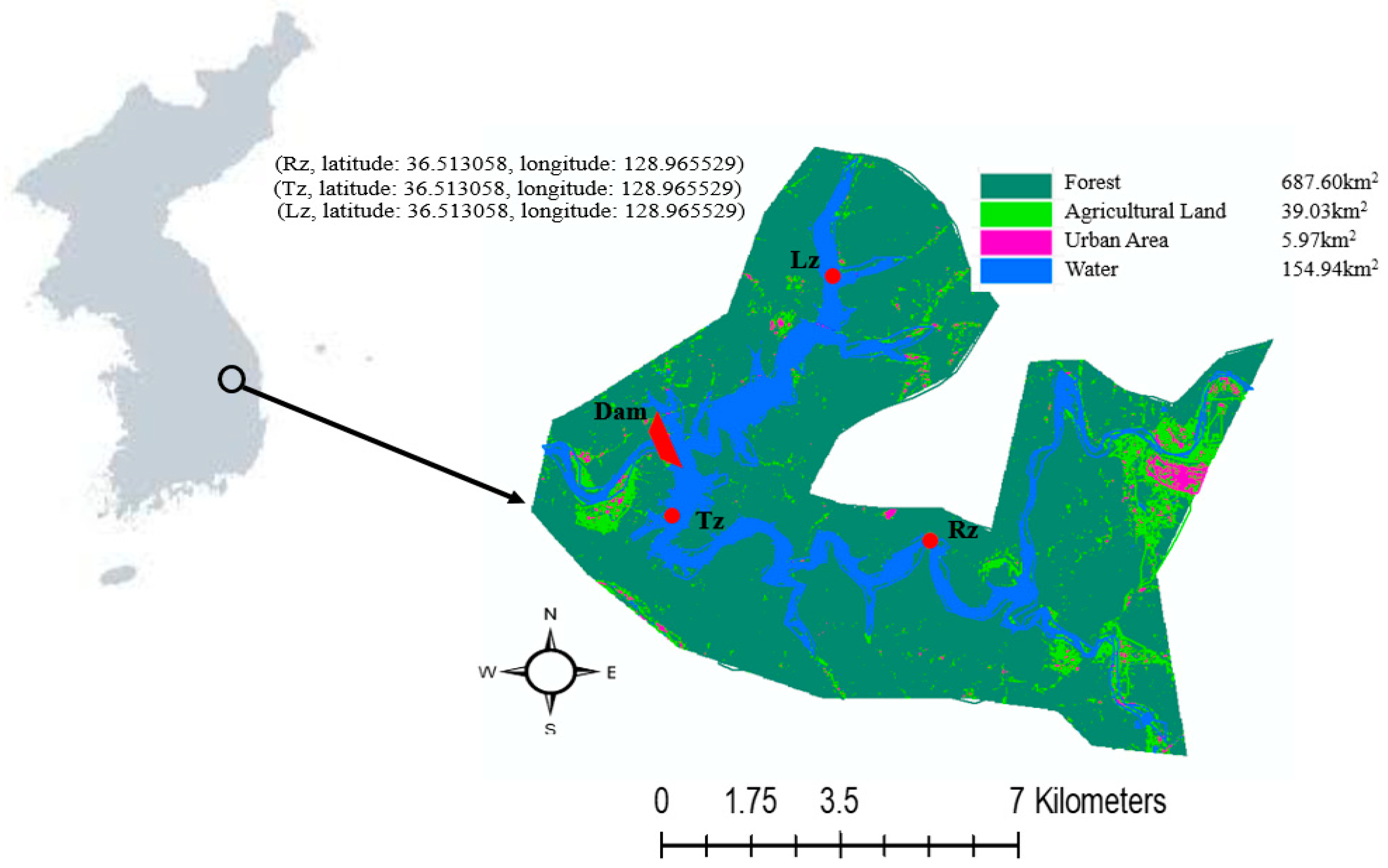
The Imha is an embankment reservoir located along the upstream section of the Nakdong River, South Korea (near Tae-Baek mountains). The study sites and land-use patterns of the reservoir have been shown in Figure 1. The catchment area of this reservoir is 1361 km2 along with 595,000,000 m3 water holding capacity [24]. In addition to that, this reservoir has a surface area of 26.4 km2 and the water level is attained at an elevation of 163 m [24]. The mean depth of the Imha reservoir is 16 m. The surface water quality parameters data (2000–2017) of Imha reservoir were collected from three different zones likes riverine zone (Rz, latitude: 36.513058, longitude: 128.965529), transitional zone (Tz, latitude: 36.513058, longitude: 128.965529) and lacustrine zone (Lz, latitude: 36.513058, longitude: 128.965529). The upstream of the reservoir (riverine zone) land is very scarce and the bed of the reservoir is composed of rock and hard homogenous granite [25]. The annual domestic and industrial water supply of the Imha reservoir is 363.6 × 10⁶ m3 [24]. Moreover, the annual irrigation water supplied by Imha reservoir is 13 × 106 m3 [24]. This artificial reservoir also facilitates flood control, helps to maintain water quality and efficient development of water resources.
2.2. Analysis of Water Quality Parameters and Rainfall Data
The monthly surface water quality parameters data were obtained from the Korean Ministry of Environment. A portable multi-parameter analyzer (YSI Sonde Model 6600) had been used to measure the electrical conductivity (EC), dissolved oxygen (DO) and water temperature (WT). The concentration of total nitrogen (TN), biological oxygen demand (BOD) and chemical oxygen demand (COD) were calculated by the chemical testing method standardized by the Ministry of the Environment, Korea [26]. Total phosphorus (TP) was measured by the ascorbic method, which is also standardized by the Ministry of the Environment, Korea [26]. Total suspended solids (TSS) and algal chlorophyll-a (CHL-a) were determined by preweighted Whatman GF/C filters method and a spectrophotometer (Bechman Model DU—65), respectively, according to the US EPA guidance (US Environmental Protection Agency, US EPA 2007) [27]. A metal disk was used to measure the transparency (SD). The monthly precipitation data were collected from the Korean Meteorological Administration at a local weather station from 2000–2017 (Gyeongsangbuk-do, Andong, Angi-dong, latitude: 36.624913, longitude: 128.715379).
2.3. Regression and Machine Learning Approaches
2.3.1. Multiple Linear Regression (MLR)
Multiple linear regression (MLR) is simply known as multiple regression, which is a statistical technique and uses several input variables (explanatory variable) to predict the outcome of a single output variable (response variable). The goal of multiple linear regression (MLR) is to model the linear relationship between the input variables and the output variable. The equation of MLR: yi = β0 + β1 xi1 + β2 xi2 + … + βp xip + ϵ (i = n observations), where, yi is the output variable, xi are input variables, β0 is the y-intercept (constant term), βp is the slope coefficients for each input variable and ε is the model’s error term (also known as the residuals).
2.3.2. Support Vector Machine (SVM)
Recently, the support vector machine (SVM) becomes more popular because of its more attractive features and pragmatic performance [28,29]. In this study, we applied support vector regression (SVR) to predict the chlorophyll-a and Secchi depth. In SVM, the SVR find a function, which estimates the difference between the input and output variable. SVM consequently estimates the function from the following equation.
where Si is the network output, Zi is the input data, which diagramed into a higher-dimensional feature via a nonlinear mapping function Φ(Zi) and wi and b are the coefficients determined by minimizing the regularized risk function based on the network output and real value [5]. A kernel function trick, radial basis function (RBF) kernel was used to predict the chlorophyll-a and Secchi depth. The RBF kernel is defined as KRBF (Z, Zi) = exp[−γ//Z − Zi//2], where γ is a parameter that sets the “spread” of the kernel.
2.3.3. Artificial Neural Network (ANN)
In recent times, artificial neural network (ANN) has paid a lot of attention for classifying patterns of multi-variable datasets and modeling complex environmental variables [5,30]. Generally, ANN consists of one or more input layers, one to many hidden layers and one output layer. The basic formula of ANN: Y = f (X, W) + €, where Y is the vector of model outputs, X is the vector of the model inputs, W is a vector of model weights and the function refers to the chosen functional relationship between outputs, inputs, and parameters of the model [31]. The chosen activation function of the network is called the sigmoid function. In the present study, for algal chlorophyll prediction, we used nine input variables and three hidden layers whereas for Secchi depth prediction ten input variables were used and three hidden layers (Supplementary Material).
2.4. K-Fold Cross-Validation and Model Accuracy Metrics
After doing the regression or building a model, we had to determine the accuracy of the model or the regression method. K-fold cross-validation (CV) is a robust method for estimating the accuracy of the model. It randomly split the dataset into K-subsets, then reserved one subset and train the model on all other subsets and repeat the process until K subsets and finally computed the average of the K recorded error. In our study, we used K = 5.
2.4.1. Mean Absolute Error
2.4.2. Root Mean Squared Error
Root mean squared error (RMSE) can also measure the average magnitude of the error [5,20]. It is the square root of the average of squared differences between prediction and real observation. Mathematically, the RMSE can be presented as the following equation. The lower the RMSE, the better the model.
2.4.3. Co-Efficient of Determination
Co-efficient of determination is the proportion of variation in the outcome that is explained by the predictor variables [5,20]. It represents the squared correlation between the observed outcome values and the predicted outcome values by the model. The higher the R2, the better the model.
where SSR is the sum of the square of residuals and SST is the total sum of squares. Sum of square residuals (SSR) is the deviations predicted from actual empirical values of data. It is a measure of the discrepancy between the data and an estimation model. A small SSR indicates a tight fit of the model to the data. It is used as an optimality criterion in parameter selection and model selection.
SST is the sum of the squares of the differences between the dependent variable and its mean.
2.5. Trophic State
The conventional criteria of USEPA (1988), based on chlorophyll-a and Secchi depth had been used for the evaluation of trophic state on the Imha reservoir [32]. The range of chlorophyll-a and Secchi depth for oligotrophic is (<4 µgL−1, >4 m), mesotrophic (4–10 µgL−1, 2–4 m), eutrophic (10–25 µgL−1, 1–2 m), and hypereutrophic (>25 µgL−1, <1 m), respectively.
2.6. Data Analysis
All kind of data analyses including MLR, SVM and ANN was done in R software (R 3.5.2 version). During the prediction of CHL-a in the reservoir using MLR, SVM and ANN, the input variable was nine (precipitation, DO, BOD, COD, TSS, TN, TP, NP ratios, WT and Cond) while it was ten variable (precipitation, DO, BOD, COD, TSS, TN, TP, NP ratios, WT, Cond and CHL-a) for the prediction of transparency (SD) in the riverine zone, transitional zone, lacustrine zone, premonsoon, monsoon and postmonsoon.
3. Results
3.1. Water Quality Summary
The physicochemical parameters of the Imha reservoir showed heterogeneity spatially and temporarily (Table 1). The maximum dissolved oxygen level has been observed in the riverine zone (17.6 mg L−1) in comparison to transitional (13.2 mg L−1) and lacustrine zone (15.4 mg L−1). The mean BOD level was highest in the lacustrine zone (2.12 mg L−1) than the riverine (2.05 mg L−1) and transitional (2.04 mg L−1) zone. The mean and maximum TSS, TN, TP, WT, Cond and CHL-a were in higher concentrations in the riverine zone compared to transitional and lacustrine zone due to surface run-off from the watershed. It is noticeable that the maximum and mean concentration of TP was found during the monsoon period due to heavy rainfall, which brings the nutrients into the Imha reservoir. During the monsoon time, the highest water temperature was also observed in the Imha reservoir.
3.2. Analysis of Hydrology Pattern
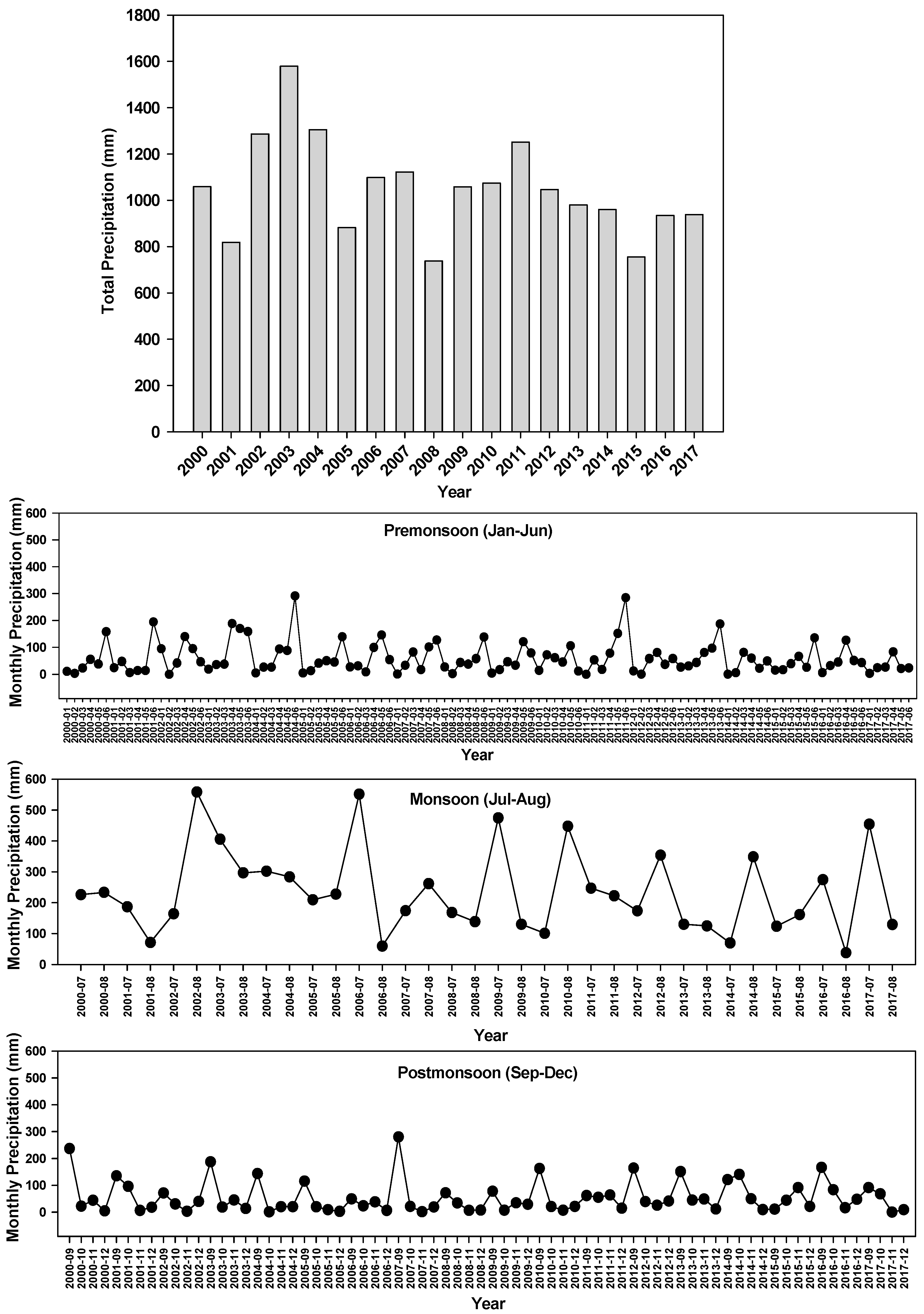
During the study, the annual and seasonal hydrology showed distinct differences from 2000–2017 (Figure 2). The weak monsoon observed during 2001 (818.1 mm), 2008 (737.9 mm) and 2015 (755.1 mm), designated as a drought year. On the contrary, the intense monsoon happened in 2002 (1286.5 mm), 2003 (1579.3 mm), 2004 (1305 mm) and 2011 (1251.5), labeled as a high flooded year. In Korea, half of the annual rainfall occurs during the monsoon period (July–August). The monsoon rainy season has been divided into two phases in the Korean peninsula; the first phase occurs in July when the rains are frequent but less intense in comparison to the second phase. The second phase starts from August to early September when occasional typhoons pass over the Korean peninsula. These typhoons are always gone along with heavier rainfall and can significantly impact the hydrological, physical, chemical and biological conditions of the ecosystem. During the premonsoon and postmonsoon, the average annual rainfall was 59.50 mm, 54.73 mm whereas it was 236.66 mm during the monsoon period.
3.3. Chlorophyll-a Prediction, Cross-Validation and Trophic State in Different Zones
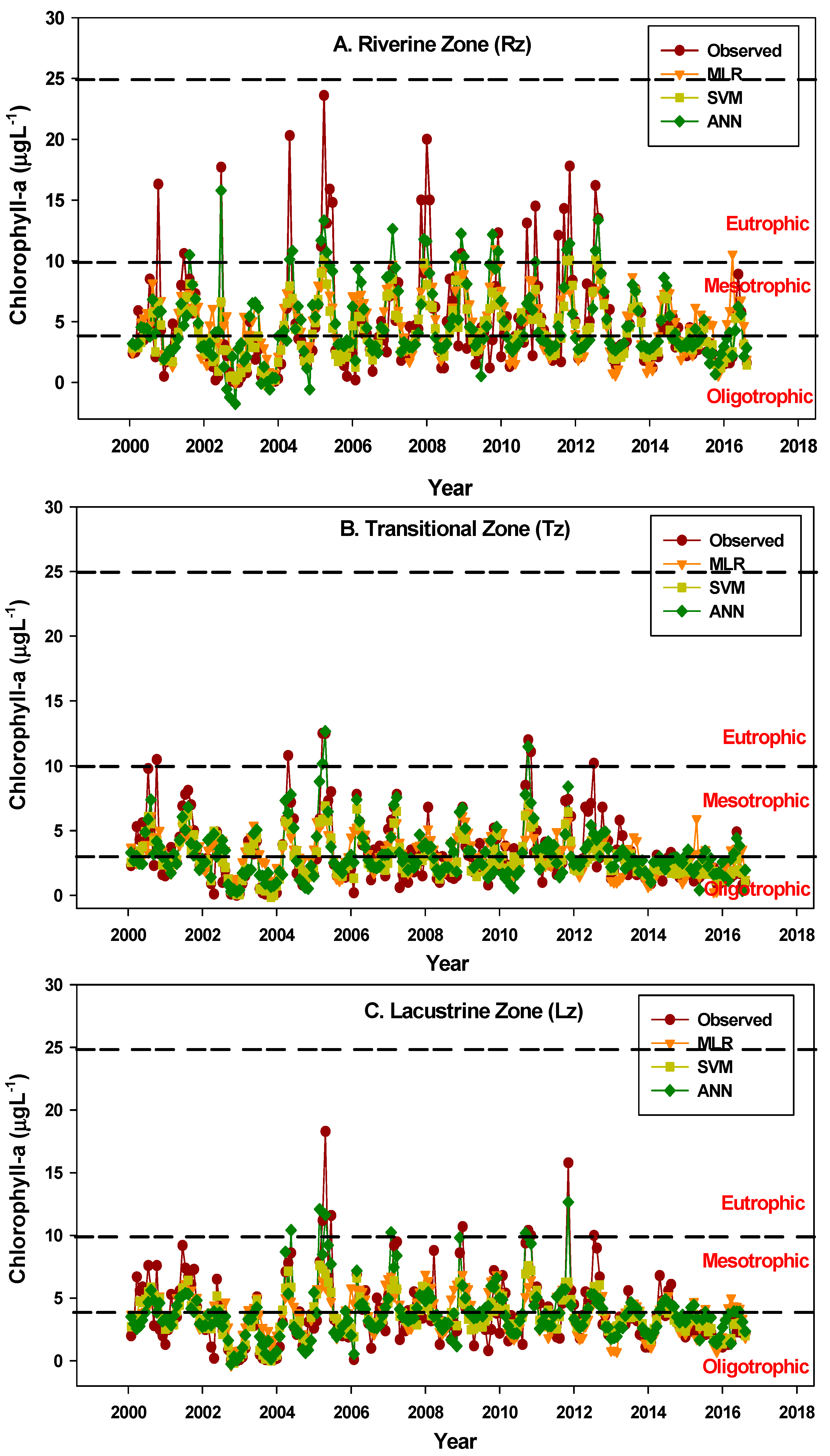
The chlorophyll-a concentration fluctuated from the riverine zone to the lacustrine zone and it was higher in the riverine zone in comparison to transitional and lacustrine zone (Figure 3). Time series plot of CHL-a in the Rz, Tz and Lz revealed that the predicted value of the SVM is closer to the observed value than ANN and MLR (Figure 3). After doing the regression by MLR, SVM and ANN, the model accuracy was evaluated by the cross-validation (CV, K = 5) approach. The modeling accuracy was quantitatively compared by the root mean square error (RMSE), coefficient of determination (R2), and mean absolute error (MAE) between the predicted and the observed Chl-a concentrations (Table 2). The RMSE was lower in Tz compared to Rz and Lz by MLR, SVM and ANN, respectively before validation (Table 2). It is noticeable that the RMSE value was 1.58 and 1.56 in Tz by SVM and ANN before validation, accordingly. After validation (CV, K = 5) the RMSE value was increased by MLR and ANN but not by SVM. The RMSE value was lower in Tz and Lz (RMSE = 1.31 and 1.59) by SVM than MLR and ANN. The R2 was the highest in Tz (R2 = 0.63) by SVM compared to ANN and MLR (R2 = 0.60 and 0.30) before validation. While the R2 value was the highest at Lz (R2 = 0.80) than Tz (R2 = 0.73) and Rz (R2 = 0.75) in SVM after validation. The maximum MAE value was observed at Rz (MAE = 3.20) in ANN after validation.
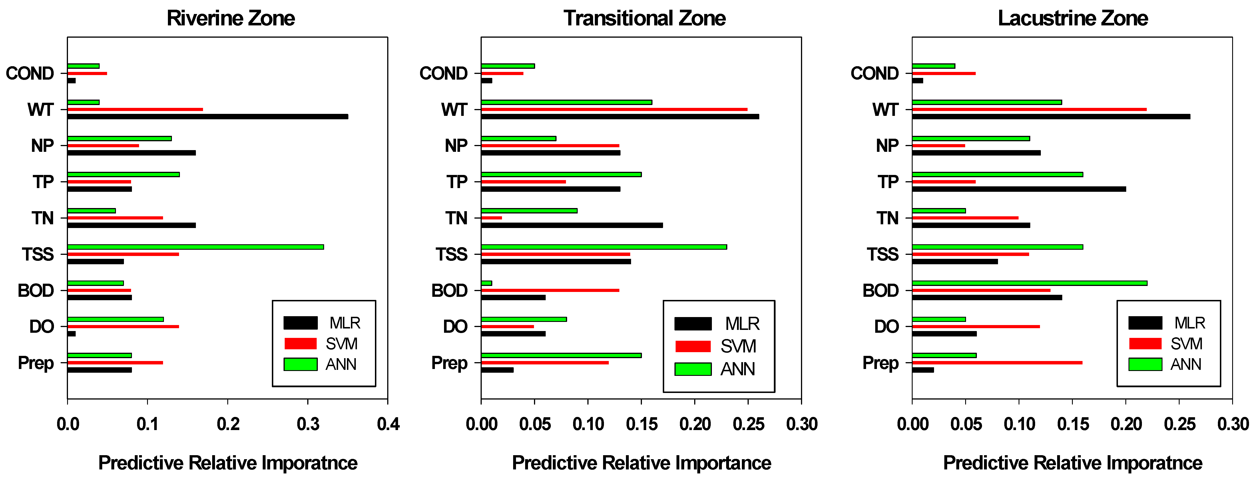
The predictive relative importance of input variables was explained in Figure 4. Based on MLR, water temperature (WT) was identified as the most important input variable, followed by total nitrogen (TN) and total nitrogen:total phosphorus (NP) ratios in Rz (Figure 3). On the contrary, the leading driver was total suspended solids (TSS) in Rz explained by SVM and ANN model. At Tz, WT was the salient variable based on MLR and SVM whereas it was TSS in ANN. The results of ANN in Lz showed that BOD was the foremost important variable.
The trophic state based on chlorophyll-a has so much fluctuated in the riverine zone compared to the transitional and lacustrine zone. The severe oligotrophic condition based on chlorophyll-a had been observed during intense flooded year (2002, 2003 and 2004) in the reservoir. In the transitional zone, the trophic state of Imha was in oligotrophic to mesotrophic conditions. It was followed by the same pattern for the lacustrine zone. In the riverine zone, the concentration of chlorophyll-a was higher and the trophic state was from oligotrophic to eutrophic over the study period.
3.4. Chlorophyll-a Prediction, Cross-Validation and Trophic State in Different Season
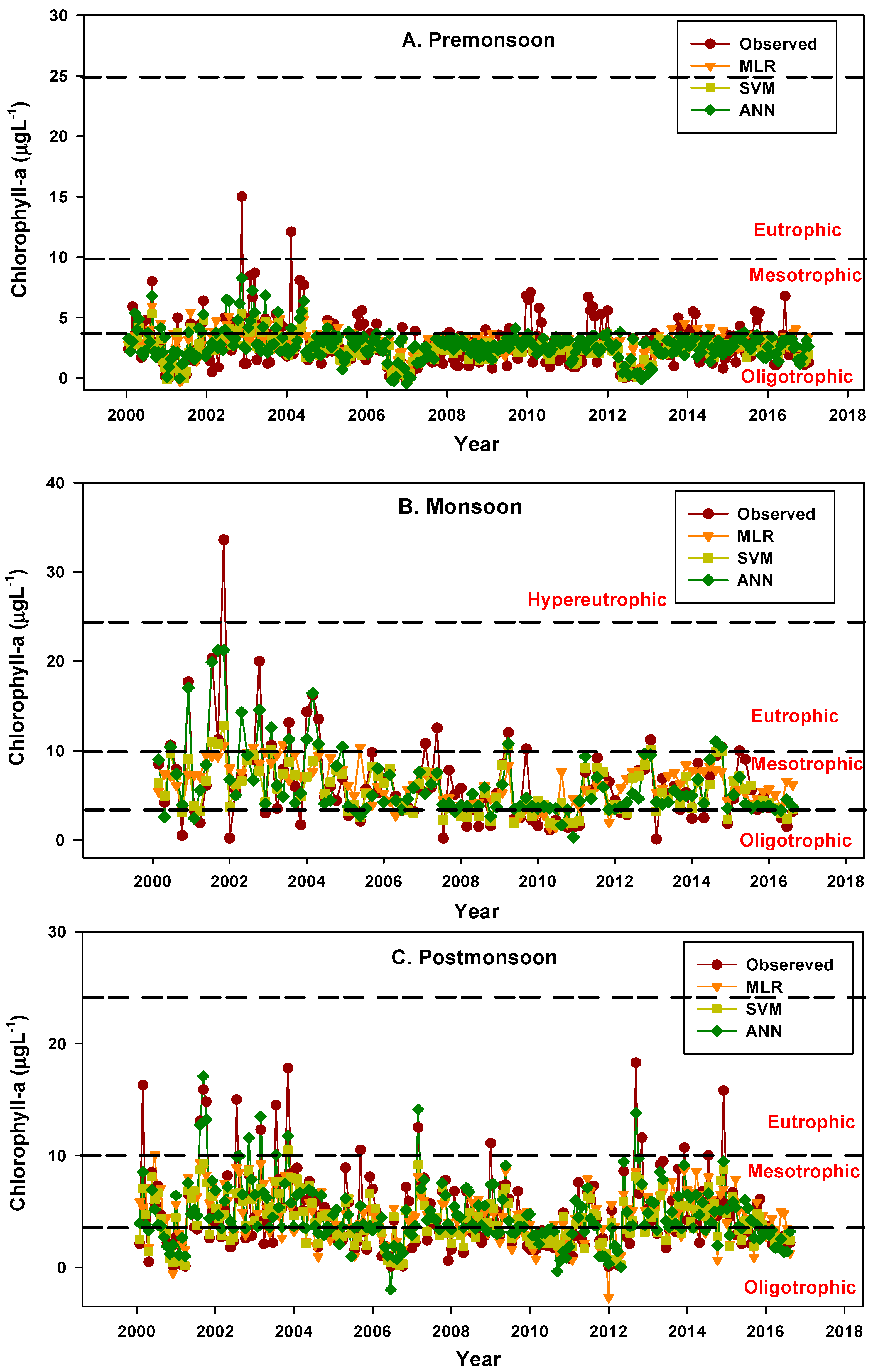
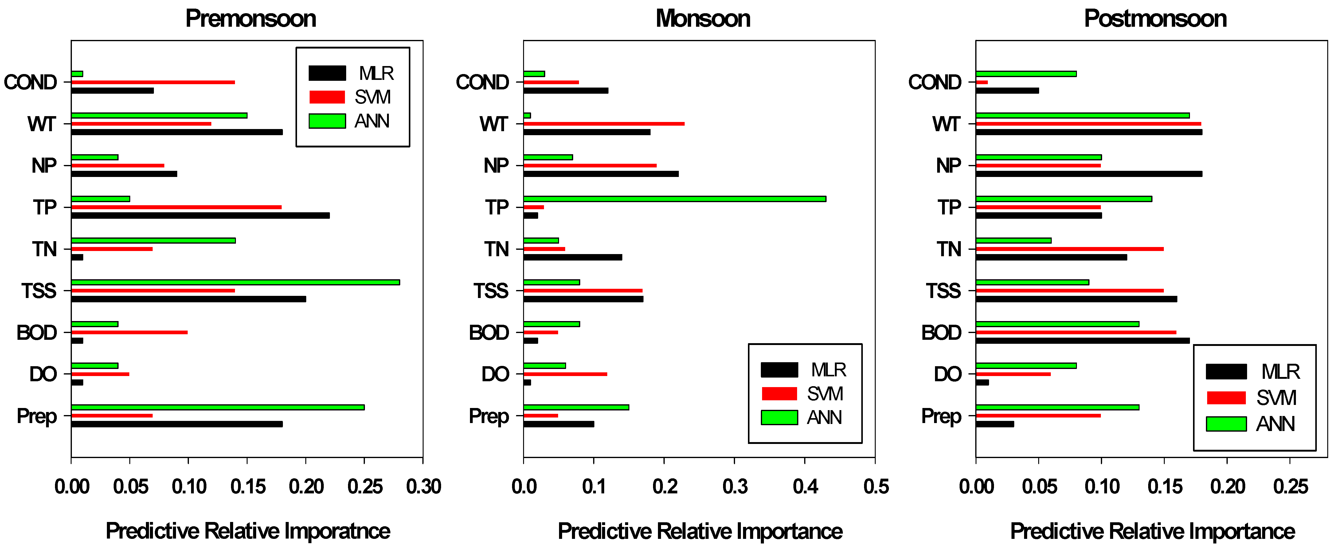
The concentration of chlorophyll-a varied seasonally and it was highest in the monsoon season compared to premonsoon and postmonsoon (Figure 5). The time series plot of observed and predicted chlorophyll-a based on MLR, SVM and ANN has been shown in Figure 5. The MLR results revealed that the root mean square (RMSE) value was the highest during the premonsoon, monsoon and postmonsoon seasons in comparison to SVM and ANN before validation (Table 3). The SVM results exhibited that the lowest RMSE value was found in premonsoon (RMSE = 1.04) compared to monsoon and postmonsoon (RMSE = 1.51 and 1.80) after validation. The R2 value was the highest during the premonsoon, monsoon and postmonsoon before and after validation by SVM than MLR and ANN. The lowest MAE value was observed in SVM than MLR and ANN at three different seasons before and after validation. In premonsoon, MLR and SVM indicated that TP was the most important predictor driver for chlorophyll-a fluctuations while ANN disclosed that it was the TSS (Figure 6). Based on the ANN model, TP was the most important input driver whereas it was the NP ratios followed by SVM and MLR in monsoon. WT was the most salient feature in MLR, SVM and ANN in postmonsoon.
During the drought year of 2001, the reservoir trophic state was in oligotrophic condition due to the lack of nutrients availability. During the premonsoon season, the reservoir showed a lower amount of chlorophyll-a growth and stated as an oligotrophic condition. The concentration of chlorophyll-a had fluctuated so much in the year of 2001, 2002 and 2003 and the trophic state was oligotrophic to hypereutrophic due to the intense summer monsoon. From 2015 to 2017, the chlorophyll-a growth had been decreasing and the trophic state going to mesotrophic to oligotrophic conditions during the monsoon and postmonsoon season.
3.5. Transparency (Secchi Depth) Prediction, Cross-Validation and Trophic State in Different Zones
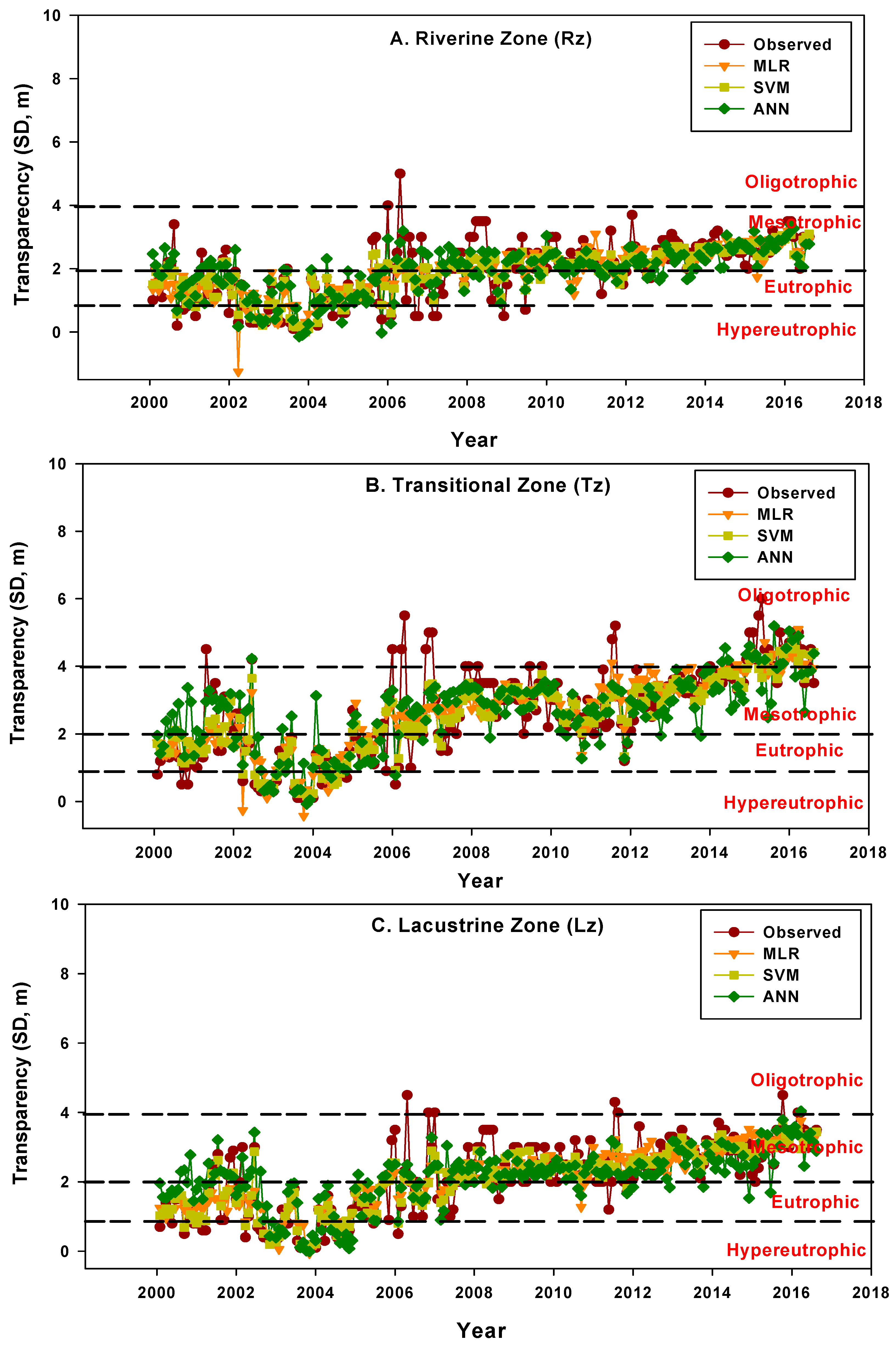
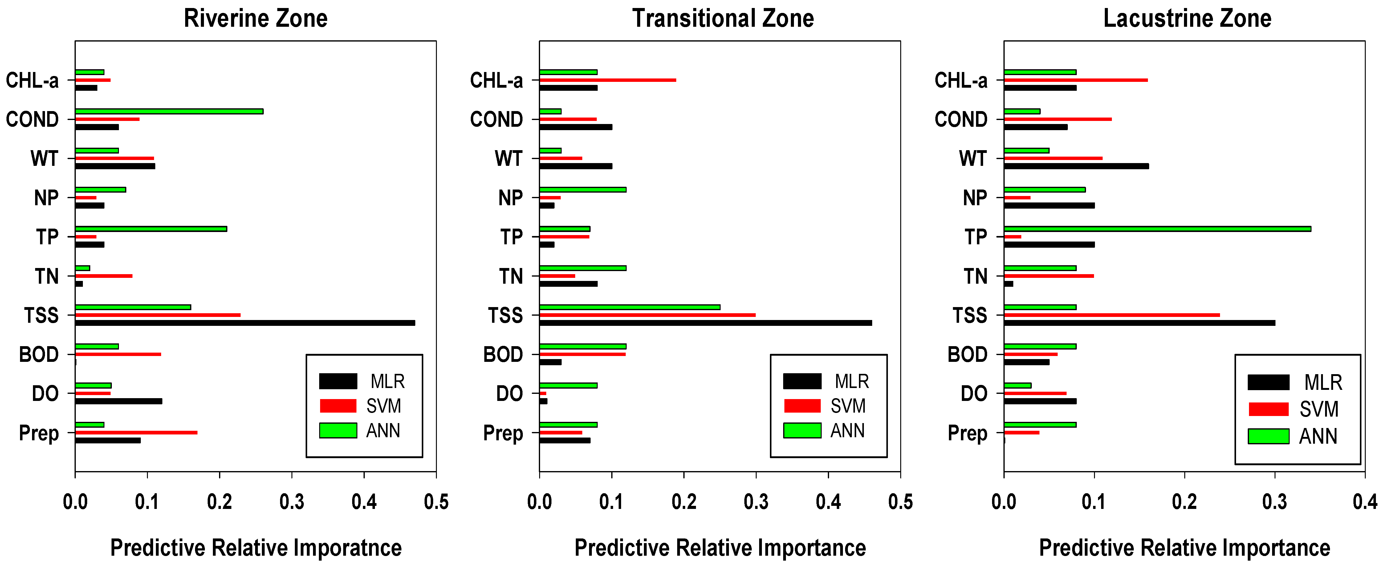
The transparency of Imha reservoir had fluctuated during the study period (Figure 7). The time series plot of observed and predicted transparency (Secchi depth) based on MLR, SVM and ANN has been shown in Figure 6. The lowest RMSE value was observed in SVM compared to MLR and ANN in three different zones at before and after validation (Rz, Tz and Lz; Table 4). The ANN model revealed that the RMSE value was the highest in Tz (RMSE = 1.49) than Rz (RMSE = 1.10) and Lz (RMSE = 1.17) after validation. The highest R2 value was found in the SVM model in Rz, Tz and Lz paralleled to MLR and ANN at after and before validation. The lowest MAE value was observed at SVM compared to another model likes MLR and ANN in Rz, Tz and Lz. It is noticeable that TSS was the most important input driver in MLR, SVM and ANN, which influenced the Secchi depth of Imha reservoir (Figure 8). The second most important input variable was TP in MLR, SVM and ANN.
The Imha reservoir had suffered immense turbidity problems during the typhoons period of 2002, 2003 and 2004. The reservoir showed hypereutrohic conditions based on Secchi depth from riverine to transitional zone. From 2006 to 2017, the trophic state of the reservoir was in eutrophic to mesotrophic conditions.
3.6. Transparency (Secchi Depth) Prediction, Cross-Validation and Trophic State in Different Season
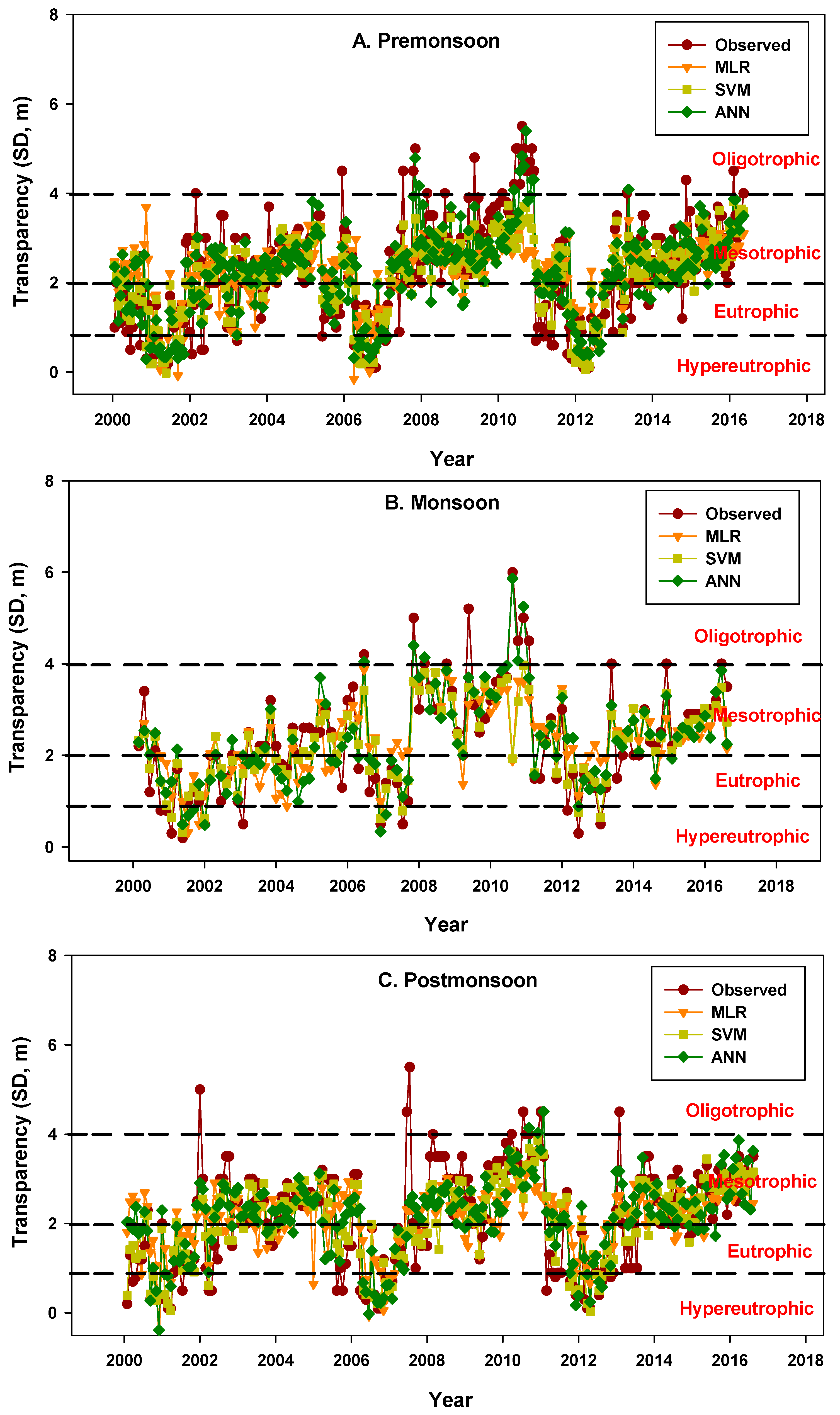
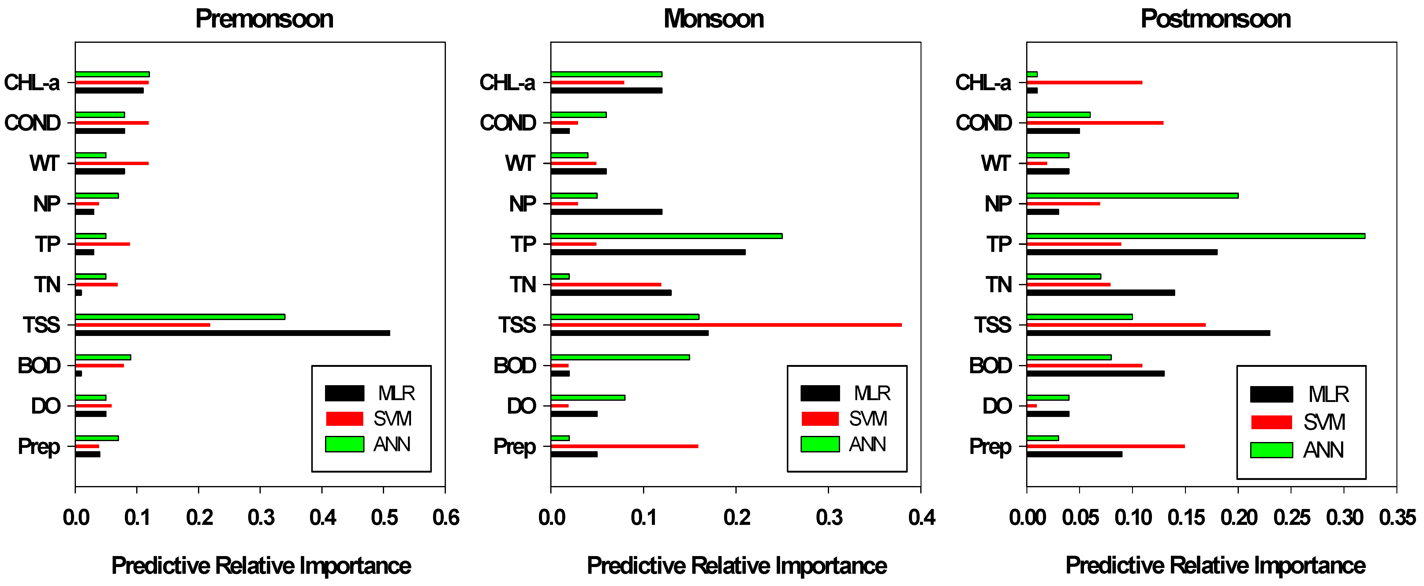
The transparency of the Imha reservoir showed seasonal variation (Figure 9). Figure 9 showed that the observed and predicted transparency (Secchi depth) time series plot based on MLR, SVM and ANN during the premonsoon, monsoon and postmonsoon season. The highest RMSE value was observed during postmonsoon by the ANN model after validation (RMSE = 1.27; Table 5). On the contrary, the lowest RMSE value was found in SVM at premonsoon (RMSE = 0.41), monsoon (RMSE = 0.39) and postmonsoon (RMSE = 0.31) after validation (Table 5). Before validation, the R2 value was highest during monsoon (R2 = 0.75) by ANN model while it was highest during postmonsoon (R2 = 0.92) by the SVM model. The minimum MAE value was observed by the SVM model in comparison to the MLR and ANN model before and after validation. The results of MLR, SVM, and ANN showed that TSS was the most important input variable, which influenced Secchi depth in the reservoir during premonsoon (Figure 10). During monsoon, the SVM model showed that TSS, Prep and TN were the important driver for Secchi depth prediction. While in the ANN model, TP was the most salient feature for Secchi depth prediction. It follows the same trend during postmonsoon by the ANN model. Based on the MLR and SVM model, TSS was the first ranked driver for the Secchi depth prediction during the postmonsoon.
The trophic state of the reservoir based on the Secchi depth varied seasonally. During premonsoon, monsoon and postmonsoon, the reservoir showed hypereutrophic conditions in the year of 2001, 2002, 2006, 2011 and 2012. Throughout the monsoon period, the trophic state of the reservoir was in mesotrophic to oligotrophic due to shorter residence time of water from 2008 to 2011.
4. Discussion
Our study showed that the SVM indicated the highest prediction accuracy for chlorophyll-a and transparency (Secchi depth) compared to MLR and ANN in Rz, Lz and TZ during premonsoon, monsoon and postmonsoon. This result concurred with the previous studies of Juam and Yeongsan reservoirs in South Korea [5]. The higher performance of SVM in comparison to MLR indicated that MLR has a highly complex of nonlinearity problems [20]. The SVM gave the better result in paralleled to ANN due to several reasons. First, SVM has a good ability to interpret of a nonlinear relationship than ANN and because of this ANN gave relatively poor accuracy [33]. Sebald and Bucklew (2000) revealed that SVM has a superior equalization performance than ANN [34]. Second, in terms of minimizing error, SVM is more effective than ANN due to the reason that SVM contains the structural risk minimization principle while ANN holds an empirical risk minimization principle [5,35]. Third, due to the inherent algorithm design of ANN, it is tough to determine optimized model parameters in comparison to SVM [36]. Fourth, due to the complex structure of ANN, the optimization of model parameters are not stable, even though the data set is the same whereas SVM has no that kind of problem [37].
In Rz, Tz and Lz, the results of MLR, SVM and ANN showed that WT was a more important predictor for chlorophyll-a than TP, TN, NP ratios and TSS. The result of the present study concurred with the previous study of a lake in China [38]. The chlorophyll-a growth was influenced by the nutrient availability (TP and TN) in Rz, Tz and Lz, which is similar to some previous studies [39,40]. The results of ANN model showed that during monsoon TP was the most important variable for chlorophyll growth in the reservoir. The present findings are similar to some recent studies [5,40]. During premonsoon, the precipitation influences the chlorophyll in the reservoir [39].
Generally speaking, transparency (Secchi depth) is influenced by watercolor, turbidity and nutrients [41,42,43]. Based on our MLR, ANN and SVM modeling approach, in different zones and season, there are three most important factors, which influence the Secchi depth in Imha Reservoir. Among these, one is total suspended solids (TSS), and two others are total phosphorus (TP) and total phosphorus:total nitrogen ratio (NP ratios). Time series of transparency clearly showed that Secchi depth had been increasing while the algal chlorophyll-a had been decreasing, which means that algal chlorophyll and transparency were inter-correlated in the reservoir system. The present findings of our study were in line with the previous studies in Taiwan, which was carried out in Te-Chi reservoir [41].
5. Summary
This research carried out different data-driven models for chlorophyll-a and transparency (Secchi depth) prediction in different zones and seasons in the reservoir. The SVM model gave a better performance than MLR and ANN in the present study. The most important input variable was WT, TSS, TP, NP ratios and precipitation, which influenced the chlorophyll-a and Secchi depth. The trophic state of the reservoir based on chlorophyll-a and Secchi depth was from mesotrophic to oligotrophic during the year of 2013 to 2017. Moreover, our present study suggests that different types of machine learning approaches should be used for further prediction of chlorophyll-a and Secchi depth in the reservoir studies.
Supplementary Materials
The following are available online at https://www.mdpi.com/2073-4441/12/1/30/s1, Figure S1: Time series plot of precipitation from 2010 to 2017, Figure S2: Structure of artificial neural network model of Rz, Tz, Lz, Pre, Mon, Postm to predict chlorophyll–a (Rz—Riverine zone, Tz—transitional zone, Lz—lacustrine zone, Pre—premonsoon, Mon—monsoon and Postm—postmonsoon), Figure S3: Structure of artificial neural network model of Rz, Tz, Lz, Pre, Mon, Postm to predict transparency (Secchi depth) (Rz—Riverine zone, Tz—transitional zone, Lz—lacustrine zone, Pre—premonsoon, Mon—monsoon and Postm—postmonsoon).
Author Contributions
M.M. conceived the idea, designed the experiments, analyzed the data, prepared the illustrations and the manuscript under the supervision of K.-G.A., J.-J.K. helped to get the data, M.A.A. helped to analyze the data. All authors have read and agreed to the published version of the manuscript.
Funding
This work was supported by “Research Fund of Chungnam National University”.
Acknowledgments
The authors are highly acknowledged to the Chungnam National University.
Conflicts of Interest
The authors have no conflict of interest.
References
- Smith, V.H. Eutrophication of freshwater and coastal marine ecosystems: A global problem. Environ. Sci. Pollut. Res. 2003, 10, 126–139. [Google Scholar] [CrossRef] [PubMed]
- Gao, C.; Zhang, T.L. Eutrophication in a Chinese context: Understanding various physical and socio-economic aspects. Ambio 2010, 39, 385–393. [Google Scholar] [CrossRef] [PubMed] [Green Version]
- Morse, N.B.; Wollheim, W.M. Climate variability masks the impacts of land use change on nutrient export in a suburbanizing watershed. Biogeochemistry 2014, 121, 45–59. [Google Scholar] [CrossRef]
- Glasgow, H.B.; Burkholder, J.M.; Reed, R.E.; Lewitus, A.J.; Kleinman, J.E. Real-time remote monitoring of water quality: A review of current applications, and advancements in sensor, telemetry, and computing technologies. J. Exp. Mar. Biol. Ecol. 2004, 300, 409–448. [Google Scholar] [CrossRef]
- Park, Y.; Cho, K.H.; Park, J.; Cha, S.M.; Kim, J.H. Development of early-warning protocol for predicting chlorophyll-a concentration using machine learning models in freshwater and estuarine reservoirs, Korea. Sci. Total Environ. 2015, 502, 31–41. [Google Scholar] [CrossRef]
- Cho, K.H.; Kang, J.H.; Ki, S.J.; Park, Y.; Cha, S.M.; Kim, J.H. Determination of the Optimal Parameters in Regression Models for the Prediction of Chlorophyll-a: A Case Study of the Yeongsan Reservoir, Korea. Sci. Total Environ. 2009, 407, 2536–2545. [Google Scholar] [CrossRef]
- Handan, C.; Nilsun, D.; Kanik, A.; Keskyn, S. Use of Principal Component Scores in Multiple Linear Regression Models for Prediction of Chlorophyll-a in Reservoirs. Ecol. Model. 2004, 181, 581–589. [Google Scholar]
- Pereira, G.C.; Evsukoff, A.; Ebecken, N.F.F. Fuzzy modelling of chlorophyll production in a brazilian upwelling system. Ecol. Model. 2009, 220, 1506–1512. [Google Scholar] [CrossRef]
- Anderson, D.M.; Andersen, P.; Bricelj, V.M.; Cullen, J.J.; Rensel, J.E. Monitoring and Management Strategies for Harmful Algal Blooms in Coastal Waters; Intergovernmental Oceanographic Commission Technical Series No. 59; APEC #201-MR-01.1; Asia Pacific Economic Program: Singapore; UNESCO: Paris, France, 2001. [Google Scholar]
- Wu, Z.; Zhang, Y.; Zhou, Y.; Liu, M.; Shi, K.; Yu, Z. Seasonal-spatial distribution and long-term variation of transparency in xin’anjiang reservoir: Implications for reservoir management. Int. J. Environ. Res. Public Health 2015, 12, 9492–9507. [Google Scholar] [CrossRef]
- Wang, F.; Wang, X.; Chen, B.; Zhao, Y.; Yang, Z. Chlorophyll a simulation in a lake ecosystem using a model with wavelet analysis and artificial neural network. Environ. Manag. 2013, 51, 1044–1054. [Google Scholar] [CrossRef]
- Kirk, J.T. Light and Photosynthesis in Aquatic Ecosystems; Cambridge University Press: Cambridge, UK, 2011. [Google Scholar]
- Karlsson, J.; Byström, P.; Ask, J.; Ask, P.; Persson, L.; Jansson, M. Light limitation of nutrient-poor lake ecosystems. Nature 2009, 460, 506–509. [Google Scholar] [CrossRef] [PubMed]
- Zhang, Y.; Wu, Z.; Liu, M.; He, J.; Shi, K.; Zhou, Y.; Wang, M.; Liu, X. Dissolved oxygen stratification and response to thermal structure and long-term climate change in a large and deep subtropical reservoir (Lake Qiandaohu, China). Water Res. 2015, 75, 249–258. [Google Scholar] [CrossRef] [PubMed]
- Jassby, A.D.; Reuter, J.E.; Goldman, C.R. Determining long-term water quality change in the presence of climate variability: Lake Tahoe (USA). Can. J. Fish. Aquat. Sci. 2003, 60, 1452–1461. [Google Scholar] [CrossRef]
- Naumenko, M.A. Seasonality and trends in the Secchi disk transparency of Lake Ladoga. In European Large Lakes Ecosystem Changes and Their Ecological and Socioeconomic Impacts; Springer: Berlin, Germany, 2008; pp. 59–65. [Google Scholar]
- Martin, S.; Soranno, P.; Bremigan, M.; Cheruvelil, K. Comparing hydrogeomorphic approaches to lake classification. Environ. Manag. 2011, 48, 957–974. [Google Scholar] [CrossRef]
- Jiang, J.; Wang, P.; Tian, Z.; Guo, L.; Wang, Y. A comparative study of statistical learning methods to predict eutriphication trendency in a resevior, northeast China. In 2011 Second International Conference on Mechanic Automation and Control Engineering; IEEE: Piscataway, NJ, USA, 2011; ISBN 978-1-4244-9439-2/11. [Google Scholar]
- Halecki, W.; Mlynski, D.; Ryczek, M.; Kruk, E.; Radecki-Pawlik, A. Applying an artificial neural network (ANN) to assess soil salinity and temperature variability in agricultural areas of a mountain catchment. Pol. J. Environ. Stud. 2017, 26, 2545–2554. [Google Scholar] [CrossRef]
- Alam, M.A.; Fukumizu, K. Hyperparameter selection in kernel principal component analysis. J. Comput. Sci. 2014, 10, 1139–1150. [Google Scholar] [CrossRef] [Green Version]
- Xie, Z.; Lou, I.; Ung, W.K.; Mok, K.M. Freshwater algal bloom prediction by support vector machine in macau storage reservoirs. Math. Probl. Eng. Vol. 2012, 2012, 397473. [Google Scholar] [CrossRef]
- Ren, Y.; Bai, G. Determination of optimal SVM parameters by using GA/PSO. J. Comput. 2010, 5, 1160–1168. [Google Scholar] [CrossRef]
- Kim, B.K.; Kim, S.; Kyung, M.S.; Lee, K.H.; Kim, H.S. Prediction of suspended sediment in Imha Reservoir, Korea. In World Environmental and Water Resources Congress 2007: Restoring Our Natural Habitat; ASCE: Reston, VA, USA, 2007. [Google Scholar]
- Ji, J.; Kim, H.; Yu, M.; Choi, C.; Yi, J.; Kang, J. Reservoir system operation using a diversion tunnel. WIT Trans. Ecol. Environ. 2014, 184, 87–98. [Google Scholar] [CrossRef] [Green Version]
- Engineering Consultation and Survey Center Central Mill Supply Co. Ltd. Feasibility Study of Hydro Sites on Nakdong River-Imha Hydroelectric Project; The Government Republic of Korea: Seoul, Korea, 1962.
- Korea Ministry of Environment. Water Pollution Investigation Method. 2001. Available online: http://Water.nier.go.kr (accessed on 19 December 2019).
- US Environmental Protection Agency. Guideline for Data Quality Assessment; USEPA: Washington, DC, USA, 2007.
- Cortes, C.; Vapnik, V. Support-vector networks. Mach. Learn. 1995, 20, 273–297. [Google Scholar] [CrossRef]
- Alam, M.A.; Fukumizu, K.; Wang, Y.P. Influence function and robust variant of kernel canonical analysis. Neurocomputing 2018, 304, 12–29. [Google Scholar] [CrossRef] [PubMed]
- Cho, K.H.; Sthiannopkao, S.; Pachepsky, Y.A.; Kim, K.W.; Kim, J.H. Prediction of contamination potential of groundwater arsenic in Cambodia, Laos, and Thailand using artificial neural network. Water Res. 2011, 45, 5535–5544. [Google Scholar] [CrossRef] [PubMed]
- Marinósdóttir, H. Applications of Different Machine Learning Methods for Water Level Predictions. Master’s Thesis, Reykjavik University, Reykjavik, Iceland, 2019. [Google Scholar]
- United States Environmental Protection Agency (USEPA). The Lake and Reservoir Restoration Guidance Manual; EPA 440/5-88-002; USEPA: Washington, DC, USA, 1988.
- Balabin, R.M.; Lomakina, E.I. Support vector machine regression (SVR/LS-SVM)—An alternative to neural networks (ANN) for analytical chemistry? Comparison of nonlinear methods on near infrared (NIR) spectroscopy data. Analyst 2011, 136, 1703–1712. [Google Scholar] [CrossRef] [PubMed]
- Sebald, D.J.; Bucklew, J.A. Support vector machine techniques for nonlinear equalization. IEEE Trans. Signal Process. 2000, 48, 3217–3226. [Google Scholar] [CrossRef]
- Kim, K.J. Financial time series forecasting using support vector machines. Neurocomputing 2003, 55, 307–319. [Google Scholar] [CrossRef]
- Chen, W.H.; Hsu, S.H.; Shen, H.P. Application of SVM and ANN for intrusion detection. Comput. Oper. Res. 2005, 32, 2617–2634. [Google Scholar] [CrossRef]
- Basu, A.; Walters, C.; Shepherd, M. Support vector machines for text categorization. In Proceedings of the IEEE 36th Annual Hawaii International Conference on System Sciences, Big Island, HI, USA, 6–9 January 2003; p. 7. [Google Scholar]
- Xia, L.; Feng, J.; Wang, Y. Chlorophyll a predictability and relative importance of factors governing lake phytoplankton at different timescales. Sci. Total Environ. 2015, 648, 472–480. [Google Scholar]
- Mamun, M.; Lee, S.J.; An, K.G. Temporal and spatial variation of nutrients, suspended solids, and chlorophyll in Yeongsan watershed. J. Asia-Pac. Biodivers. 2018, 11, 206–216. [Google Scholar] [CrossRef]
- Atique, U.; An, K.G. Reservoir water quality assessment based on chemical parameters and the chlorophyll dynamics in relation to nutrient regime. Pol. J. Environ. Stud. 2019, 28, 1–19. [Google Scholar] [CrossRef]
- Kuo, J.T.; Hsieh, M.H.; Lung, W.S.; She, N. Using artificial neural network for reservoir eutrophication prediction. Ecol. Model. 2007, 200, 171–177. [Google Scholar] [CrossRef]
- Calderon, M.S.; An, K.G. An influence of mesohabitat structures (pool, riffle, and run) and land-use pattern on the index of biological integrity in the Geum River watershed. J. Ecol. Environ. 2016, 40, 1–13. [Google Scholar] [CrossRef] [Green Version]
- Ingole, N.P.; An, K.G. Modifications of nutrient regime, chlorophyll-a, and trophic state relations in Daechung Reservoir after the construction of an upper dam. J. Ecol. Environ. 2016, 40, 1–10. [Google Scholar] [CrossRef] [Green Version]
Figure 1.
The map showing sampling sites of Imha reservoirs, which are located at the east part of South Korea (Rz—riverine zone, Tz—transitional zone; intake tower for the drinking water supply for the citizens and Lz—lacustrine zone).
Figure 1.
The map showing sampling sites of Imha reservoirs, which are located at the east part of South Korea (Rz—riverine zone, Tz—transitional zone; intake tower for the drinking water supply for the citizens and Lz—lacustrine zone).

Figure 2.
The monthly and annual precipitation pattern in the Imha reservoir from 2000–2017.

Figure 3.
Chlorophyll-a time series plot of the riverine, transitional and lacustrine zone in Imha reservoirs based on observed data, MLR, SVM and ANN model (MLR—multiple linear regression, SVM—support vector machine, ANN—artificial neural network). (A) Riverine zone (Rz), (B) Transitional zone (Tz), (C) Lacustrine zone (Lz).

Figure 4.
The predictive relative importance of input variables for chlorophyll-a prediction based on MLR, SVM and ANN model in Rz, Tz and Lz.
Figure 4.
The predictive relative importance of input variables for chlorophyll-a prediction based on MLR, SVM and ANN model in Rz, Tz and Lz.

Figure 5.
Chlorophyll-a time series plot of premonsoon, monsoon and postmonsoon of Imha reservoirs based on observed data, MLR, SVM and ANN model (MLR—multiple linear regression, SVM—support vector machine, ANN—artificial neural network). (A) Premonsoon, (B) Monsoon, (C) Postmonsoon.
Figure 5.
Chlorophyll-a time series plot of premonsoon, monsoon and postmonsoon of Imha reservoirs based on observed data, MLR, SVM and ANN model (MLR—multiple linear regression, SVM—support vector machine, ANN—artificial neural network). (A) Premonsoon, (B) Monsoon, (C) Postmonsoon.

Figure 6.
The predictive relative importance of input variable for chlorophyll-a prediction based on MLR, SVM and ANN model during premonsoon, monsoon and postmonsoon.
Figure 6.
The predictive relative importance of input variable for chlorophyll-a prediction based on MLR, SVM and ANN model during premonsoon, monsoon and postmonsoon.

Figure 7.
Transparency (Secchi depth) time series plot of riverine, transitional and lacustrine zone of Imha reservoirs based on observed data, MLR, SVM and ANN model (MLR—multiple linear regression, SVM—support vector machine, ANN—artificial neural network). (A) Riverine Zone, (Rz), (B) Transitional Zone (Tz), (C) Lacustrine Zone (Lz).

Figure 8.
Predictive relative importance of input variable for transparency (Secchi depth) prediction based on MLR, SVM and ANN model in RZ, Tz and Lz.
Figure 8.
Predictive relative importance of input variable for transparency (Secchi depth) prediction based on MLR, SVM and ANN model in RZ, Tz and Lz.

Figure 9.
Transparency (Secchi depth) time series plot of premonsoon, monsoon and postmonsoon of Imha reservoirs based on observed data, MLR, SVM and ANN model (MLR—multiple linear regression, SVM—support vector machine, ANN—artificial neural network). (A) Premonsoon, (B) Monsoon, (C) Postmonsoon.
Figure 9.
Transparency (Secchi depth) time series plot of premonsoon, monsoon and postmonsoon of Imha reservoirs based on observed data, MLR, SVM and ANN model (MLR—multiple linear regression, SVM—support vector machine, ANN—artificial neural network). (A) Premonsoon, (B) Monsoon, (C) Postmonsoon.

Figure 10.
Predictive relative importance of input variable for transparency (Secchi depth) prediction based on MLR, SVM and ANN model in premonsoon, monsoon and postmonsoon.
Figure 10.
Predictive relative importance of input variable for transparency (Secchi depth) prediction based on MLR, SVM and ANN model in premonsoon, monsoon and postmonsoon.


Table 1.
Summary of Imha reservoir water quality parameters based on the riverine zone (Rz, n = 216), transitional zone (Tz, n = 216) and lacustrine zone (Lz, n = 216) Lz, and premonsoon (January–June, n = 319), monsoon (July–August, n = 108) and postmonsoon (September–December, n = 216), SD = standard deviation, CV = coefficient of variation, min = minimum and max = maximum.
| Water Quality Parameters | Riverine Zone Mean ± SD (Min–Max) (CV) | Transitional Zone Mean ± SD (Min–Max) (CV) | Lacustrine Zone Mean ± SD (Min–Max) (CV) | Premonsoon Mean ± SD (Min–Max) (CV) | Monsoon Mean ± SD (Min–Max) (CV) | Postmonsoon Mean ± SD (Min–Max) (CV) |
|---|---|---|---|---|---|---|
| DO (mg/L) | 8.70 ± 2.16 (2.1–17.6) (24.82) | 7.91 ± 2.13 (3.1–13.2) (26.92) | 8.50 ± 2.21 (2.8–15.4) (26) | 9.58 ± 1.71 (3.2–15.4) (17.84) | 7.17 ± 1.91 (2.6–17.6) (26.63) | 7.16 ± 1.96 (2.1–11.5) (27.37) |
| BOD (mg/L) | 2.05 ± 0.49 (1.2–4) (23.90) | 2.04 ± 0.51 (1.2–3.6) (25) | 2.12 ± 0.50 (1.2–4) (23.58) | 2.0 ± 0.52 (1.2–4) (26) | 2.12 ± 0.40 (1.2–3.2) (18.86) | 2.16 ± 0.50 (1.3–4) (23.14) |
| TSS (mg/L) | 4.51 ± 3.67 (0.5–36) (81.37) | 3.70 ± 1.63 (0.2–19) (44.05) | 3.91 ± 2.90 (0.5–14.4) (74.16) | 3.54 ± 3.63 (0.2–36) (102.54) | 4.98 ± 3.40 (0.5–15.4) (68.27) | 4.31 ± 2.70 (0.3–14.6) (62.64) |
| TN (mg/L) | 1.69 ± 0.41 (0.79–2.99) (24.26) | 1.63 ± 0.39 (0.80–3.37) (23.92) | 1.63 ± 0.42 (0.73–2.85) (25.76) | 1.63 ± 0.40 (0.79–3.38) (24.53) | 1.77 ± 0.45 (1.03–2.85) (25.42) | 1.63 ± 0.38 (0.73–2.66) (23.31) |
| TP (mg/L) | 0.03 ± 0.01 (0.009–0.17) (33.33) | 0.027 ± 0.01 0.01–0.10 (37.03) | 0.028 ± 0.01 (0.01–0.14) (35.71) | 0.025 ± 0.007 (0.01–0.057) (28) | 0.035 ± 0.02 (0.015–0.174) (57.14) | 0.03 ± 0.01 (0.01–0.138) (33.33) |
| NP ratios | 65.10 ± 23.66 (14.36–179.33) (36.34) | 67.55 ± 25.27 (13.77–169.28) (37.40) | 64.20 ± 23.66 (10.85–165.75) (36.85) | 70.23 ± 24.06 (21.25–169) (34.25) | 61.57 ± 25.01 (13.77–158.83) (40.62) | 60.85 ± 22.84 (10.85–179.33) (37.53) |
| WT (°C) | 14.09 ± 7.59 (2–29) (53.86) | 10.13 ± 4.42 (3–19) (43.63) | 13.31 ± 6.88 (2–27) (51.69) | 8.02 ± 4.89 (2–23) (60.97) | 19.36 ± 4.75 (9.8–29) (24.53) | 15.69 ± 4.65 (7–25.4) (29.63) |
| Cond. (µs/cm) | 177.42 ± 61.91 (57–404) (34.88) | 163.62 ± 61.29 (4–312) (37.40) | 168.85 ± 57.28 (83–322) (33.87) | 168.69 ± 67.80 (4–404) (40.19) | 184.25 ± 49.60 (114–332) (26.91) | 164.60 ± 52.20 (86–316) (31.71) |
| CHL-a (µg/L) | 4.80 ± 4.19 (1.8–23.6) (87.29) | 3.18 ± 2.49 (0.1–12.5) (78.30) | 3.82 ± 2.74 (0.1–18.3) (71.72) | 2.68 ± 1.86 (0.1–15) (69.14) | 6.23 ± 4.91 (0.47–4.91) (78.81) | 4.65 ± 3.45 (0.1–18.3) (74.19) |
| SD (m) | 1.89 ± 0.96 (0.1–5) (50.79) | 2.62 ± 1.34 (0.1–6) (51.14) | 2.12 ± 1.05 (0.1–4.5) (49.52) | 2.22 ± 1.18 (0.1–5.5) (53.15) | 2.33 ± 1.17 (0.2–6) (50.21) | 2.12 ± 1.15 (0.1–5.5) (54.24) |
Table 2.
Model accuracy metrics of Rz, Tz and Lz for chlorophyll-a prediction on the basis of MLR, SVM and ANN (Rz—riverine zone, Tz—transitional zone, Lz—lacustrine zone, MLR—multiple linear regression, SVM—support vector machine, ANN—artificial neural network).
Table 2.
Model accuracy metrics of Rz, Tz and Lz for chlorophyll-a prediction on the basis of MLR, SVM and ANN (Rz—riverine zone, Tz—transitional zone, Lz—lacustrine zone, MLR—multiple linear regression, SVM—support vector machine, ANN—artificial neural network).
| Model Accuracy Metrics | Riverine Zone (Rz) | Transitional Zone (Tz) | Lacustrine Zone (Lz) | |||||||||||||||
|---|---|---|---|---|---|---|---|---|---|---|---|---|---|---|---|---|---|---|
| Before Validation | After Validation | Before Validation | After Validation | Before Validation | After Validation | |||||||||||||
| MLR | SVM | ANN | MLR | SVM | ANN | MLR | SVM | ANN | MLR | SVM | ANN | MLR | SVM | ANN | MLR | SVM | ANN | |
| RMSE | 3.37 | 2.86 | 2.83 | 3.61 | 2.57 | 4.96 | 2.07 | 1.58 | 1.56 | 2.18 | 1.31 | 2.93 | 2.25 | 1.77 | 1.72 | 2.31 | 1.59 | 3.40 |
| R2 | 0.34 | 0.56 | 0.53 | 0.28 | 0.75 | 0.43 | 0.30 | 0.63 | 0.60 | 0.26 | 0.73 | 0.40 | 0.31 | 0.58 | 0.60 | 0.25 | 0.80 | 0.40 |
| MAE | 2.30 | 1.52 | 1.96 | 2.49 | 1.24 | 3.20 | 1.54 | 0.96 | 1.15 | 1.62 | 0.62 | 1.98 | 1.65 | 1.07 | 1.28 | 1.73 | 0.68 | 2.25 |
Table 3.
Model accuracy metrics of premonsoon, monsoon and postmonsoon for chlorophyll-a prediction based on MLR, SVM and ANN (MLR—multiple linear regression, SVM—support vector machine, ANN—artificial neural network).
Table 3.
Model accuracy metrics of premonsoon, monsoon and postmonsoon for chlorophyll-a prediction based on MLR, SVM and ANN (MLR—multiple linear regression, SVM—support vector machine, ANN—artificial neural network).
| Model Accuracy Metrics | Premonsoon (January–June) | Monsoon (July–August) | Postmonsoon (September–December) | |||||||||||||||
|---|---|---|---|---|---|---|---|---|---|---|---|---|---|---|---|---|---|---|
| Before Validation | After Validation | Before Validation | After Validation | Before Validation | After Validation | |||||||||||||
| MLR | SVM | ANN | MLR | SVM | ANN | MLR | SVM | ANN | MLR | SVM | ANN | MLR | SVM | ANN | MLR | SVM | ANN | |
| RMSE | 1.60 | 1.35 | 1.42 | 1.64 | 1.04 | 1.99 | 4.34 | 3.25 | 2.85 | 4.77 | 1.51 | 6.04 | 2.65 | 2.15 | 2.09 | 2.83 | 1.80 | 4.88 |
| R2 | 0.25 | 0.50 | 0.41 | 0.23 | 0.71 | 0.37 | 0.20 | 0.57 | 0.65 | 0.10 | 0.81 | 0.27 | 0.40 | 0.62 | 0.63 | 0.34 | 0.77 | 0.48 |
| MAE | 1.15 | 0.81 | 1.04 | 1.19 | 0.40 | 1.29 | 3.09 | 1.73 | 2.10 | 3.37 | 0.78 | 3.78 | 1.98 | 1.26 | 1.64 | 2.14 | 0.80 | 2.59 |
Table 4.
Model accuracy metrics of Rz, Tz and Lz for transparency (Secchi depth) prediction on the basis of MLR, SVM and ANN (Rz—riverine zone, Tz—transitional zone, Lz—lacustrine zone, MLR—multiple linear regression, SVM—support vector machine, ANN—artificial neural network).
Table 4.
Model accuracy metrics of Rz, Tz and Lz for transparency (Secchi depth) prediction on the basis of MLR, SVM and ANN (Rz—riverine zone, Tz—transitional zone, Lz—lacustrine zone, MLR—multiple linear regression, SVM—support vector machine, ANN—artificial neural network).
| Model Accuracy Metrics | Riverine Zone (Rz) | Transitional Zone (Tz) | Lacustrine Zone (Lz) | |||||||||||||||
|---|---|---|---|---|---|---|---|---|---|---|---|---|---|---|---|---|---|---|
| Before Validation | After Validation | Before Validation | After Validation | Before Validation | After Validation | |||||||||||||
| MLR | SVM | ANN | MLR | SVM | ANN | MLR | SVM | ANN | MLR | SVM | ANN | MLR | SVM | ANN | MLR | SVM | ANN | |
| RMSE | 0.63 | 0.50 | 0.60 | 0.87 | 0.29 | 1.10 | 0.77 | 0.64 | 0.82 | 1.10 | 0.40 | 1.49 | 0.63 | 0.47 | 0.69 | 0.92 | 0.33 | 1.17 |
| R2 | 0.55 | 0.72 | 0.59 | 0.24 | 0.90 | 0.49 | 0.66 | 0.77 | 0.62 | 0.32 | 0.90 | 0.50 | 0.63 | 0.79 | 0.56 | 0.26 | 0.90 | 0.47 |
| MAE | 0.48 | 0.32 | 0.46 | 0.67 | 0.19 | 0.81 | 0.59 | 0.39 | 0.62 | 0.87 | 0.27 | 1.24 | 0.49 | 0.30 | 0.52 | 0.73 | 0.23 | 0.92 |
Table 5.
Model accuracy metrics of premonsoon, monsoon and postmonsoon for transparency (Secchi depth) prediction based on MLR, SVM and ANN (MLR—multiple linear regression, SVM—support vector machine, ANN—artificial neural network).
Table 5.
Model accuracy metrics of premonsoon, monsoon and postmonsoon for transparency (Secchi depth) prediction based on MLR, SVM and ANN (MLR—multiple linear regression, SVM—support vector machine, ANN—artificial neural network).
| Model Accuracy Metrics | Premonsoon (January–June) | Monsoon (July–August) | Postmonsoon (September–December) | |||||||||||||||
|---|---|---|---|---|---|---|---|---|---|---|---|---|---|---|---|---|---|---|
| Before Validation | After Validation | Before Validation | After Validation | Before Validation | After Validation | |||||||||||||
| MLR | SVM | ANN | MLR | SVM | ANN | MLR | SVM | ANN | MLR | SVM | ANN | MLR | SVM | ANN | MLR | SVM | ANN | |
| RMSE | 0.88 | 0.61 | 0.69 | 0.95 | 0.41 | 1.01 | 0.85 | 0.62 | 0.57 | 1.00 | 0.39 | 1.18 | 0.94 | 0.65 | 0.79 | 1.01 | 0.31 | 1.27 |
| R2 | 0.43 | 0.72 | 0.65 | 0.40 | 0.87 | 0.57 | 0.46 | 0.71 | 0.75 | 0.37 | 0.87 | 0.53 | 0.32 | 0.67 | 0.53 | 0.24 | 0.92 | 0.47 |
| MAE | 0.68 | 0.42 | 0.56 | 0.71 | 0.23 | 0.80 | 0.66 | 0.37 | 0.44 | 0.80 | 0.21 | 0.78 | 0.76 | 0.40 | 0.62 | 0.82 | 0.19 | 1.27 |
© 2019 by the authors. Licensee MDPI, Basel, Switzerland. This article is an open access article distributed under the terms and conditions of the Creative Commons Attribution (CC BY) license (http://creativecommons.org/licenses/by/4.0/).
Share and Cite
MDPI and ACS Style
Mamun, M.; Kim, J.-J.; Alam, M.A.; An, K.-G. Prediction of Algal Chlorophyll-a and Water Clarity in Monsoon-Region Reservoir Using Machine Learning Approaches. Water 2020, 12, 30. https://doi.org/10.3390/w12010030
AMA Style
Mamun M, Kim J-J, Alam MA, An K-G. Prediction of Algal Chlorophyll-a and Water Clarity in Monsoon-Region Reservoir Using Machine Learning Approaches. Water. 2020; 12(1):30. https://doi.org/10.3390/w12010030
Chicago/Turabian StyleMamun, Md, Jung-Jae Kim, Md Ashad Alam, and Kwang-Guk An. 2020. "Prediction of Algal Chlorophyll-a and Water Clarity in Monsoon-Region Reservoir Using Machine Learning Approaches" Water 12, no. 1: 30. https://doi.org/10.3390/w12010030
Note that from the first issue of 2016, this journal uses article numbers instead of page numbers. See further details here.