Distribution Coefficient and Metal Pollution Index in Water and Sediments: Proposal of a New Index for Ecological Risk Assessment of Metals

Abstract

The Lake of Texcoco is a closed basin with soils that confer salinity, conductivity, and alkalinity to it. It has undergone a reduction in size, incorporation of wastewater, and short-term desiccation, and includes temporary wetlands interconnected during the rainy season, some of which receive treated wastewater. Sediments contain metals, thus affecting water quality. Five artificial lakes were studied, and 12 metals (As, Ba, Cd, Cu, Cr, Fe, Mg, Mn, Hg, Ni, Pb, and Zn) were monitored bimonthly in water and sediments from June 2015 to March 2018. The Metal Pollution Index (MPI) and the Distribution Coefficient (Kd) were computed. Fe and Cd were the most and least stable metals in sediments, respectively (mean Log(Kd) = 4.24 and 2.079). Based on Log(K_d), metals were ranked as Fe > Mn > Zn > Cu > Mg > Cr > Ni > Ba > Pb > Hg > As > Cd. Log(K_d) values < 3 and > 5 indicate that metals occur mainly in water and sediments, respectively. The Mean Distribution Coefficient Log(K_{d MPI}) is a novel index proposed to assess ecological risk from metals in a water body. This index allows determining the phase (liquid or solid) where metals predominate, negatively affecting either free-swimming or benthic organisms. Log(K_{d MPI}) values indicated that metals occur primarily in the liquid phase in all lakes studied.

1. Introduction

Metal pollution is a global environmental issue [1], being one of the most serious and conspicuous problems in water bodies [2,3,4,5]. In fact, the world currently faces complex water management challenges associated with an increasing human population and a changing climate [6]. In the intertropical region, where many developing countries are located, the combination of accelerated population growth, industrialization, and changes in land use and land cover exerts strong pressure on water resources [7]; pollution by metals can be particularly severe. Metals are natural components of the lithosphere and also occur in aquatic sediments. Under certain biogeochemical processes, dissolution, and the effect of factors such as pH, redox potential, salinity, and hardness, among others, metals can be released to the overlying water, polluting it [8,9,10] and exposing free-swimming and benthic organisms. Metals are not degradable; they bioaccumulate and are biomagnified through the trophic web [11]. Large amounts of metals derived from anthropogenic sources such as urban, agricultural, and industrial areas are discharged into aquatic environments [5], then transported through the water column and accumulated in sediments, thus posing an ecological risk to benthic organisms, fish, and other aquatic organisms, and ultimately affecting humans [8,12].

Lakes are among the most vulnerable and fragile aquatic ecosystems, because they function as sinks for a wide range of dissolved and particulate substances [13]. Sediments are essential components of lakes, providing food for benthic organisms and accumulating multiple pollutants such as pesticides; additionally, sediments are the most important reservoirs of metals in aquatic systems [1,10,14]. Over the past three decades, metals in water and sediments of freshwater ecosystems have been the focus of interest of several researchers [15,16,17]. Therefore, the development of evaluation methods to monitor metal pollution is essential.

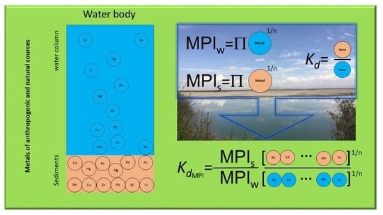
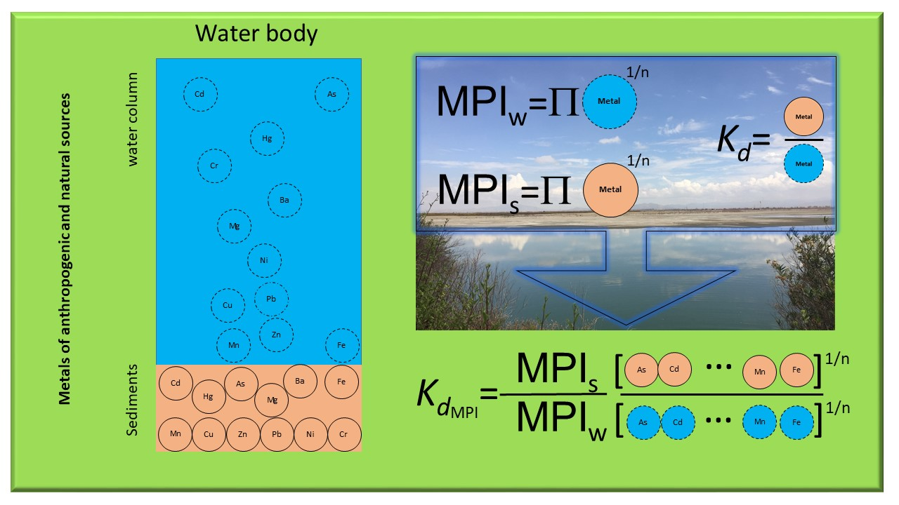
1.1. Metal Pollution Index

The Metal Pollution Index [18] is a mathematical model that summarizes the values for all metals in a single figure, calculated as the geometric mean of values for the metals considered, as follows:

$$\mathrm{MPI}={\left[{\prod }_{\mathrm{i}=1}^{\mathrm{n}}{\mathrm{Cf}}_{\mathrm{i}}\right]}^{1/\mathrm{n}}.$$

(1)

where MPI is the Metal Pollution Index, Cf_i is the concentration of the ith metal, and n is the number of metals analyzed. The MPI does not use reference concentrations, either from safety sheets, reference sites, or baselines [19]. Moreover, MPI is not expressed in a scale or as categories that indicate the pollution level; nonetheless, since it highlights those study sites with high metal concentrations, it allows making comparisons between study sites or monitoring a given site through time.

Given that MPI provides a geometric mean of metal concentrations for each water body, it is considered to be an indicator of the pollution level from these elements. Some metals occur at extremely low levels in nature or polluting sources (trace), while others may be abundant. The assessment of geometric mean values is useful for eliminating extre values that may skew the interpretation of data [19].

The global assessment of metal concentrations can be a gross indicator of pollution; however, MPI provides no information about the potential mobility of metals across the two major compartments in a water body: solid and liquid phases [10]. The mobility, fate, and bioavailability of metals are directly related to the partitioning between suspended solids, sediments, and water [4].

1.2. Distribution Coefficient

The distribution coefficient (or partition coefficient) is one of the key parameters for assessing the potential migration of a pollutant in the liquid phase that is in contact with sediment or suspended matter. This tool describes in quantitative terms the partitioning of an element or compound between sediments and the water column [20,21]. The distribution coefficient (K_d) is the ratio of pollutant concentrations between sediments and water, and is calculated by the following equation [17]:

$${\mathrm{K}}_{\mathrm{d}}=\frac{\left[{\mathrm{Metal}}_{\mathrm{S}}\right]}{\left[{\mathrm{Metal}}_{\mathrm{W}}\right]}\left[\frac{\mathrm{L}}{\mathrm{kg}}\right].$$

(2)

where K_d (L/kg) is the distribution coefficient, Metal_s is the concentration of the pollutant in sediments (mg/kg), and Metal_w is the concentration of the pollutant in water (mg/L).

K_d is affected by multiple factors such as pH, organic matter content, and salinity, all related to the nature of the water body [4]. According to [22], K_d provides crucial information for risk assessment. Log(K_d) > 5 indicate elements or compounds with affinity to bind or remain in the solid phase (sediments); values in the range 3 < Log(K_d) < 4 correspond to elents or compounds released from the solid phase (towards the liquid phase); and Log(K_d) < 3 indicate chemicals prevailing in the liquid phase.

MPI and K_d are two indices that allow evaluating metal-related pollution in a water body. MPI represents the geometric mean concentration of metals in a given compartment of the water body, either water, sediments, or both; K_d indicates the compartment where individual metals are contained. When used together, these two parameters support risk assessment for the aquatic biota [5,10,16,18,22,23].

1.3. Saline Lakes

Large saline lakes account for 44% of the volume and 23% of the area of all lakes on Earth, mostly located in arid, endorheic basins. Many saline lakes worldwide are shrinking at alarming rates, reducing waterbird habitat, leading to economic losses, and threatening human health [6]. There are few studies on metals in saline lake sediments [24,25]. Particularly, saline continental lakes are sensitive to metal pollution because sediments from hypersaline ecosystems are considered sinks and sources of trace elements [24].

The former Lake of Texcoco, in the endorheic basin of Mexico, is one of a few saline water bodies of Mexico [19,26], maybe the most important from a cultural standpoint. The lake is located in a zone with Solonchak and Vertisol soil types [27] (Figure 1). As indicated by [6], the Lake of Texcoco is part of an endorheic basin; historically, this water body has undergone multiple modifications, including reduction in size, incorporation of wastewater, and temporary desiccation. It currently comprises natural and artificial wetlands that are temporarily interconnected during the rainy season (June–October). Some of these receive treated wastewater and serve to regulate storm water floods [26]; consequently, water quality has deteriorated. In addition to human intervention on the Lake of Texcoco, Solonchak soils are natural sources of metals such as Fe, Mn, Cr, and Zn [28]. Therefore, the Lake of Texcoco, in its current state, represents a study model to monitor the presence of metals and the compartments where these are contained; in addition, a few studies have addressed metal pollution using both indices (MPI and K_d) [5] in temperate—but not in tropical—water bodies. This study aims to evaluate the concentration of metals in five water bodies of the Lake of Texcoco system, Mexico, using the MPI in water and sediments, and calculating the distribution coefficient. Based on the information provided by each index, the MPI_S/MPI_W ratio is proposed to calculate the Mean Distribution Coefficient (K_{d MPI}) for water bodies as a novel index to assess the ecological risk by metals and other xenobiotics that may potentially migrate from the liquid to the solid phase of a water body, and vice versa.

2. Materials and Methods

2.1. Study Area

The Lake of Texcoco, in a closed basin known as the “basin of Mexico”, is located in the southern portion of the Mesa Central (Mexico’s Central Plateau) and to the East of the Trans-Mexican Volcanic Belt, and is surrounded by high mountains [29]. This basin is a volcano-tectonic depression formed since the Cretaceous (with limestone recorded as the oldest rocks in the basin), and was filled by volcanic materials produced in three events: the first, during the Eocene-Oligocene and Miocene; the second, in the Miocene; and the third, in the Pliocene and late Pleistocene, associated with the early activity of the Trans-Mexican Volcanic Belt (with volcanic rocks predominating) [30]. The drainage of the basin, which flowed southward, was closed in the early Pleistocene, giving rise to a large single lake that stretched across most of the basin (80%); however, in episodic periods, this lake became fragmented into smaller reservoirs: a freshwater lake (Xochimilco) to the south of the basin and the saline Texcoco to the north. In an island within the Lake of Texcoco, the pre-Hispanic city of Tenochtitlan was founded by the Aztecs and flourished between 1325 and 1521. This lacustrine city included a system of canals and causeways, which were the earliest anthropic modifications to these lakes. When the Aztecs arrived in 1325, the basin of Mexico comprised four interconnected water bodies: Zumpango, Xaltocan, Texcoco, and Xochimilco. During the pre-Hispanic period, the basin was an extensive marshland surrounded by pine and oak forests in the highlands [31]. Tenochtitlán was destroyed during the Spanish conquest and the Lake of Texcoco was gradually drained; today, the only remnants of the lake are isolated water bodies or wetlands [32]. Mexico City, one of the megacities in the world, is located surrounding the remnants of the former Lake of Texcoco at a mean altitude of 2240 m a.s.l. The main anthropic alteration after the Spanish conquest includes pollution by municipal and industrial wastewater, desiccation for flood control, and intensive changes in land use resulting from human settlements around the lakes [33].

The Lake of Texcoco has Solonchak and Vertisol soil types, which influence the salinity, conductivity, and alkalinity of lake water. The climate is temperate semi-arid with warm summers, classified as BS Kw [34]. Maximum mean temperatures range between 30 and 32 °C from April to June, alternating with cold winters with minimum temperatures of 2 to 5 °C from October to March. Precipitation (460–600 mm/yr) is distributed mainly from June to September. Substantial evaporation rates are recorded from March to May, when little precipitation occurs [3].

Five artificial shallow lakes were studied in the area of the former Lake of Texcoco: Nabor Carrillo, Recreativo, Regulación Horaria, Fusible, and Churubusco, to assess metal pollution (Figure 1). Some of these water bodies store and regulate effluents from a wastewater treatment facility, in addition to increasing water storage capacity and thus serving as storm water regulators [26]. The depth of these water bodies range from 0.6 m (Recreativo) to 3.5 m (Nabor Carrillo), with a surface area ranging from 0.26 km² (Recreativo) to 9.19 km² (Nabor Carrillo). The survey was carried out at bimonthly intervals from June 2015 to March 2018. In each water body, conductivity was measured in situ with a digital portable device EC/pH/T (Conductronic PC 18). In each study site, water and sediment samples were collected in duplicate. Water samples were collected at 0.2 to 0.3 m depth in polyethylene bottles, 100 ± 50 m from the edge of each water body. Surface sediment samples (top 5 cm) were collected using a plastic spatula and transferred to plastic bags. Samples were stored in coolers and transported to the laboratory. Samples were processed according to the guidelines in International and Mexican standards [35,36,37,38]. Hardness (Ethylenediaminetetraacetic acid titration method) and Total Dissolved Solids (gravimetric method) were determined according to the Mexican standards NMX-AA-072-SCFI-2001 and NMX-AA-034-SCFI-2015, respectively [39,40].

2.2. Analytical Procedure for Metals

Twelve metals were assessed (As, Ba, Cd, Cu, Cr, Fe, Mg, Mn, Hg, Ni, Pb, and Zn) in water samples and the leachable fraction of surface sediment samples from each water body. Partial digestion was performed following the modified EPA 3051 A method as reported by [41]: 45 mL aliquots of water and 0.5 g of dry sediment were placed in polytetrafluoroethylene (PFA) beakers and mixed with 2.5 mL HNO₃, 0.8 ml HCl and 1 mL H₂O₂ (all analytical grade) at 119 ± 1.5 °C and 20 psi for 40 min in an autoclave. Subsequently, the digested sediment samples were filtered on Whatman paper no. 41. All samples were placed in 50 mL volumetric flasks. Metals were tested on an atomic absorption spectrophotometer (Agilent Technologies, Spectra AA 240 FS Agilent® following the methodology in the Mexican standard NMX-051-SCFI-2001) [42]. Water samples were diluted to avoid interference due to changes in viscosity and surface tension due to high content of total dissolved solids as is indicate by [43]. High purity standards for Quality Control were used to prepare the calibration curve (ICP-200.7-6 Solution A), and to verify metal recovery (SRM No. 691029 Loam Soil B for sediments and CWW-TM-B for water). Metals recovery ranged from 91.44–111.07% ($\overline{X}$ = 101.60% ± 0.07).

2.3. Index Assessment

MPI was calculated for water (MPI_W) and sediment (MI_S) samples using Equation (1). The results are expressed as average by water body and study period. Distribution Coefficient values were calculated using Equation (2) for each metal and water body. The results are expressed as average log (K_d) by water body and study period.

2.4. Statistical Analysis

The Shapiro-Wilk test was used to assess the normality of MPI and K_d data. When data showed a normal distribution, one-way analysis of varianza (ANOVA, α = 0.05) and Tukey’s multiple comparison tests were used; otherwise, Kruskal-Wallis and Dunn’s multiple comparison tests were used. Hierarchical Cluster Analyses by Euclidean Distance (UPGMA) were conducted to identify groups based on MPI and Log(K_d) values. A discriminant multivariate analysis was performed considering Log(K_d) by metal as variable, and lakes and study periods as a priori groups. A second Hierarchical Cluster Analysis by Euclidean Distance (UPGMA) was carried out to identify groups based on Log(K_d) values by metal and water body. All statistical analyses were performed using the software XlStat version 2015.

3. Results

3.1. Chemical Characteristics of Lakes

The five artificial lakes studied are located in the area of the former Lake of Texcoco and have a Solonchak soil type as substrate (Figure 1). Therefore, lakes are influenced by various mineral salts that increase parameters such as conductivity, hardness, and total dissolved solids (TDS). The mean values of these three parameters during the study period are shown in

Table 1. Chemical characteristics of lakes in terms of conductivity, hardness, and total dissolved solids.

Water Body	Conductivity (µS/cm)		Hardness (mg/L as CaCO3)		TDS (mg/L)
	$\overline{\mathit{X}}$	±SE	$\overline{\mathit{X}}$	±SE	$\overline{\mathit{X}}$	±SE
Churubusco	2036	187	237	8	3705	1387
Regulación Horaria	4882	547	226	11	2767	372
Fusible	6397	1291	214	33	6939	2616
Recreativo	19,660	340	240	22	42,594	8037
Nabor Carrillo	6654	493	245	22	5088	1016

. Recreativo was the water body with peak conductivity values, while Churubusco exhibited the lowest. In terms of hardness, all water bodies are classified as either moderately hard or hard [44]. Similar to conductivity, Recreativo was the water body with the highest TDS, and Regulacion Horaria showed the lowest values of this parameter.

Metal concentrations in water bodies of the Lake of Texcoco system showed spatial and temporal variations associated with the nature of the substrate, the rainy and dry seasons, and the tributaries draining into each water body (some of them carrying wastewater). During the study period, the content (µg/L; mean ± standard deviation) of each metal in water samples was: As = 4.52 ± 3.6, Ba = 253.98 ± 37.5, Cd = 25.01 ± 31.04, Cr = 48.98 ± 11.59, Cu = 29.4 ± 19.0, Fe = 757.36 ± 315.20, Hg = 1.18 ± 0.14, Mg = 35176 ± 8445, Mn = 76.7 ± 37.9, Ni = 117.5 ± 145, Pb = 166.2 ± 163.4, and Zn = 50 ± 12.7. The content of each metal (mg/g; mean ± standard deviation) in sediment samples was: As = 0.46 ± 0.06, Ba = 156 ± 30, Cd = 1.94 ± 0.32, Cr = 52 ± 34, Cu = 86 ± 77, Fe = 14427.96 ± 2630.90, Hg = 1.066 ± 0.66, Mg = 29052.51 ± 11584.2, Mn = 484.6 ± 105.1, Ni = 37.9 ± 6.15, Pb = 56.59 ± 9.41, and Zn = 180.57 ± 115.38. Data by water body and metal are shown in

Table 2. Mean values of metal concentration in water and sediments samples of study lakes of Texcoco Lake System, compared with values for other shallow lakes.

Water Body	Water (µg/L)
	As	Ba	Cd	Cu	Cr	Fe	Mg	Mn	Hg	Ni	Pb	Zn
Churubusco	1.81	239	9	21	40	717	29,029	130	0.99	26	75	41
Regulación Horaria	2.13	234	9	16	46	866	27,854	57	1.24	46	97	41
Fusible	9.64	251	17	34	45	1212	31,176	89	1.10	100	112	62
Recreativo	7.14	319	80	61	69	639	47,469	80	1.37	381	458	65
Nabor Carrillo	1.85	226	9	15	44	353	40,353	28	1.20	34	90	39
Manzala Lake			20	55							22	311
Maharlu Lake			0.28	0.28		10,400	313,200	1500		2.36	5	370
Rift Valley Lakes			17	33	85			161		145	171	86
Yangtze Lakes	26	81		0.90	11			39	0.32	1.30	24	3
Water Body	Sediments (ppm)
	As	Ba	Cd	Cu	Cr	Fe	Mg	Mn	Hg	Ni	Pb	Zn
Churubusco	0.51	122	2.26	210	104	12,833	13,862	551	2.15	45	56	356
Regulación Horaria	0.37	174	1.61	25	22	11,789	38,959	329	0.44	30	47	86
Fusible	0.42	140	2.28	57	41	15,162	42,112	538	1.02	38	70	139
Recreativo	0.47	198	1.89	108	67	18,578	23,275	580	1.08	42	61	236
Nabor Carrillo	0.55	144	1.66	29	26	13,777	27,055	423	0.64	34	48	86
Maharlu Lake	0.52		3	38	40	19,477		554		207	160	67
Rift Valley Lakes			0.64	10	3			1320		25	20	169
Yangtze Lakes	31	583		465	65			837	0.03	33	46	144
Wadi El Natrum			27	45				377		26	52	45
Austria Lakes	3	141			32	1.18				44		70
Mongolian lakes	13			25	243			696		151	16	65

. Likewise, Table 2 shows comparative values for other water bodies: Manzala Lake in Egypt (water) [45], Lake Maharlu in Iran (water and sediments) [46]; Rift Valley Lakes in Kenya [47]; Lakes of the Yangtze river region in China (sediments) [48]; Wadi El Natrum Lakes in Egypt (sediments) [24]; Lakes of Eastern Austria (sediments) [49]; and Lakes of the Gobi Desert Region, Eastern Mongolia (Sediments) [50].

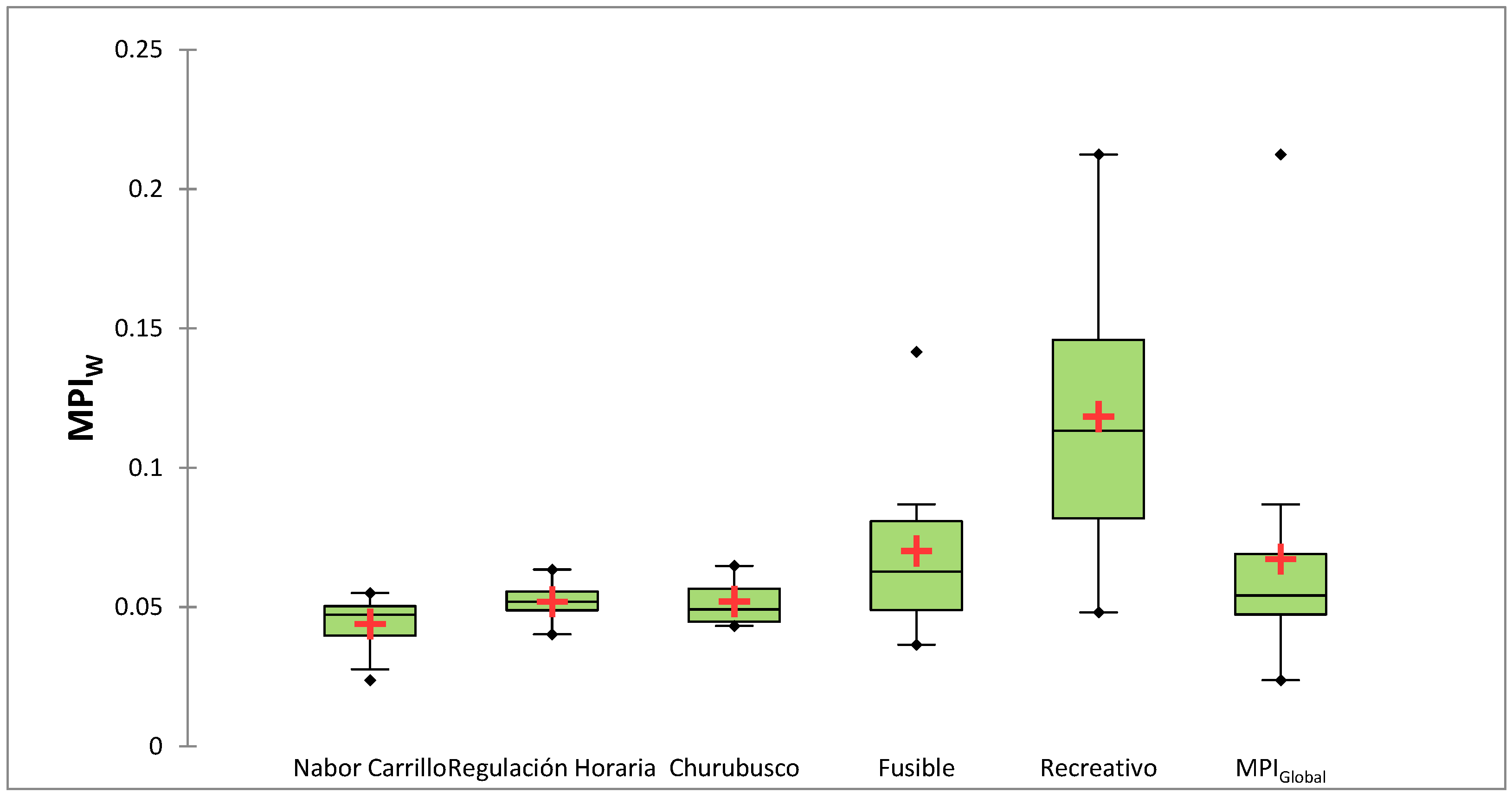
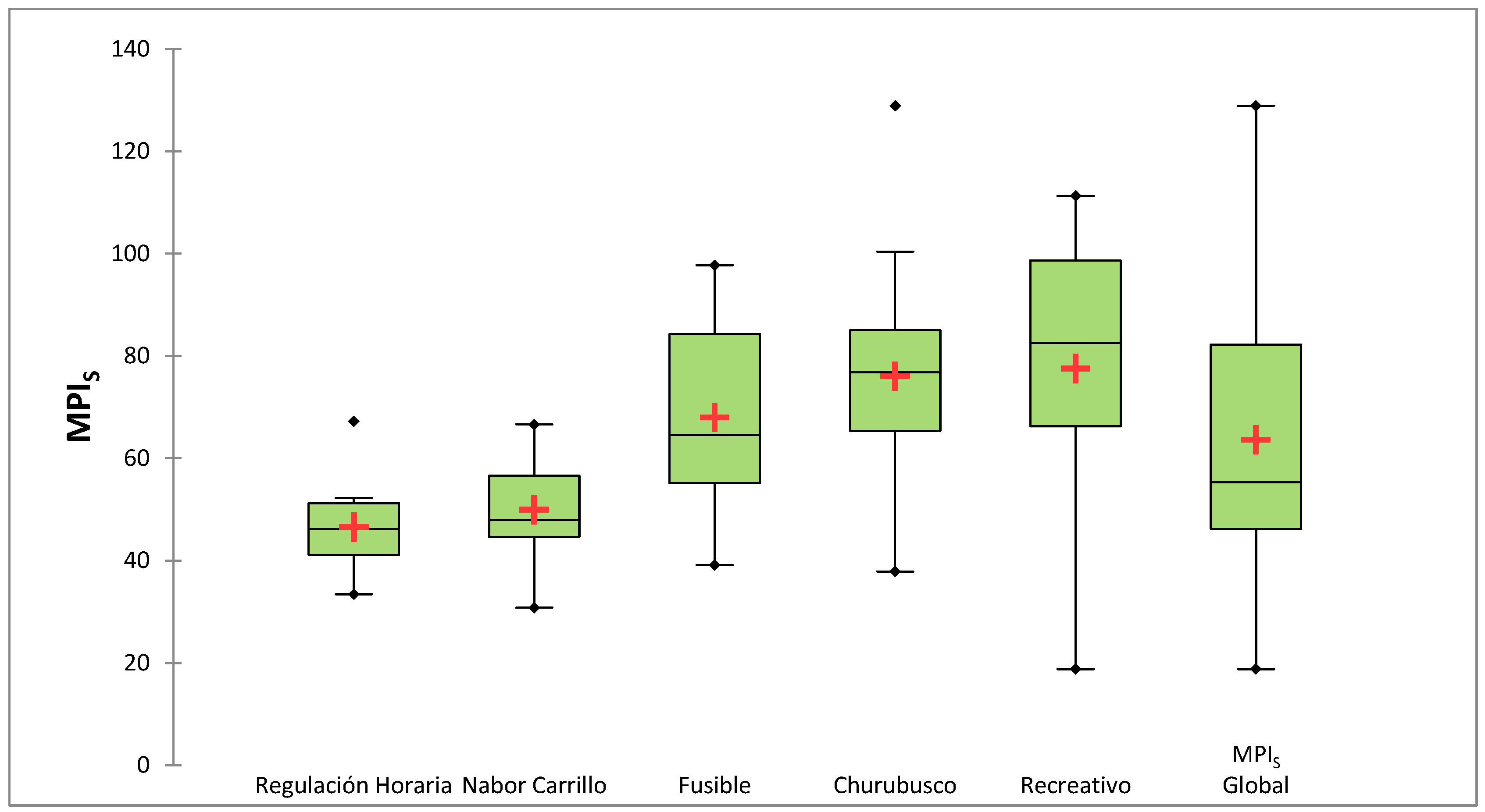
3.2. Metal Pollution Index

MPI_W values ranged from 0.024 to 0.212 during the study period, showing differences in content across water bodies. The overall mean MPI_W for all water-bodies was 0.067 (Global MPI_W). Nabor Carrillo showed the lowest MPI_W (0.044), while Recreativo showed the highest MPI_W (0.212), as well as the greatest dispersion of data, indicating that it shows the greatest fluctuations in metal concentration through time (Figure 2).

A gradient of MPI_W values was observed across water bodies in the following ranking order: Recreativo > Fusible > Churubusco > Regulación Horaria > Nabor Carrillo (Figure 2). Since data did not follow a normal distribution (Shapiro-Wilk p < 0.05), a Kruskal-Wallis test was run followed by a Dunn’s multiple comparison test to identify significant differences across water bodies. Recreativo showed highly significant differences (Dunn’s p < 0.0004) versus Churubusco, Regulación Horaria, and Nabor Carrillo. Fusible showed significant differences (Dunn’s p < 0.005) versus Nabor Carrillo (Figure 2).

MPI_S also showed a gradient across water bodies, with values ranging from 33.43 to 128.19 during the study period. Regulación Horaria showed the lowest mean MPI_S (46.5), while Recreativo showed the highest mean MPI_S (77.5) and a large data dispersion. The overall mean MPI_S considering all water bodies was 63.61 (Figure 3).

The ranking of water bodies based on MPI_S is Recreativo > Churubusco > Fusible > Nabor Carrillo > Regulación Horaria (Figure 3). Recreativo also shows the highest metal concentration in sediments. Significant differences were observed between Recreativo and Churubusco relative to Regulación Horaria and Nabor Carrillo (Dunn’s p < 0.0003), and between Regulation Horaria and Fusible (Dunn’s p < 0.001).

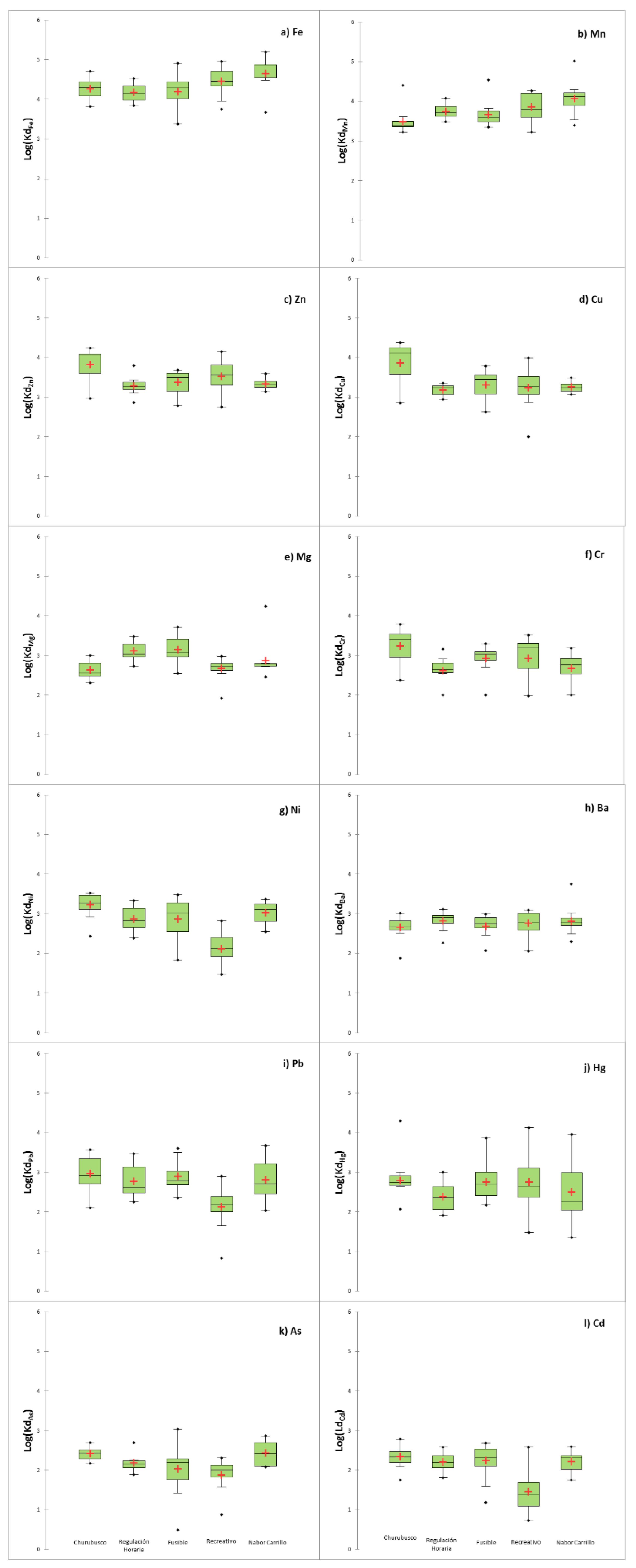
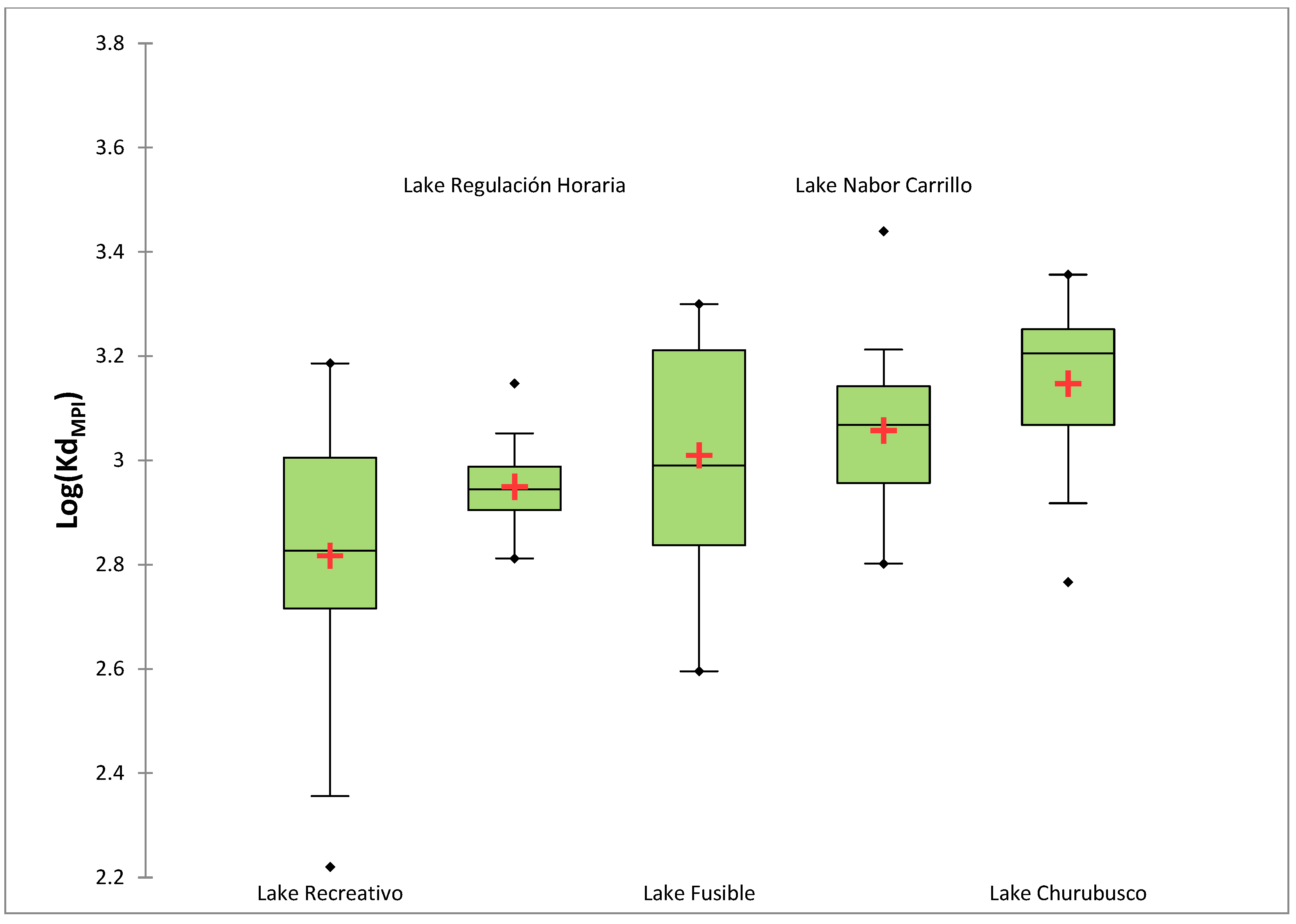
3.3. Distribution Coefficient

Log(K_{d Fe}) ranged from 3.38 (Fusible) to 5.19 (Nabor Carrillo) and showed significant differences between Nabor Carrillo and Regulación Horaria (p = 0.001) (Figure 4a). Likewise, Log(K_{d Mn}) ranged from 0.5 (Churubusco) to 3.7 (Nabor Carrillo). For its part, Log(K_{d Mn}) showed significant differences between several water bodies: Churubusco versus Regulación Horaria (p = 0.004), Recreativo (p < 0.0004), and Nabor Carrillo (p < 0.0001); and Nabor Carrillo versus Fusible (p = 0.003) (Figure 4b).

Churubusco showed significant differences in Log(K_{d Zn}) relative to Regulación Horaria (p < 0.001) and Nabor Carrillo (p < 0.005) (Figure 4c). Log (K_{d Cu}) showed significant differences between Churubusco and Regulación Horaria (p < 0.001) (Figure 4d). Churubusco showed significant differences in Log(K_{d Cr}) versus Nabor Carrillo (p < 0.0001) (Figure 4d,e). Log (K_{d Ni}) showed significant differences between Recreativo and any other lake (p < 0.05) (Figure 4f).

Log (K_{d Ba}) and Log (K_{d Hg}) showed no significant differences across water bodies (p > 0.05) (Figure 4g). Log(K_{d Pb}) for Churubusco showed significant differences versus Carrillo (p < 0.004) and Fusible (p < 0.001). Log(K_{d As}) showed significant differences for Recreativo relative to Churubusco and Nabor Carrillo (p < 0.0001) (Figure 4h). Finally, Log(K_{d Cd}) showed significant differences in Lake Recreativo versus all other lakes p ≤ 0.05) (Figure 4l).

On the other hand, As and Cd showed the lowest Log(K_d) values in all water bodies. Significant differences between water bodies based on Log(K_d) values are shown in

Table 3. Significant differences between water bodies based on K_d values by metal.

		Churubusco	Regulación Horaria	Fusible	Recreativo
Kd Fe	Churubusco
	Regulación Horaria
	Fusible
	Recreativo
	Nabor Carrillo		0.001
Kd Mn	Churubusco
	Regulación Horaria	<0.004
	Fusible
	Recreativo	<0.0005
	Nabor Carrillo	<0.0001		0.003
Kd Zn	Churubusco
	Regulación Horaria	<0.001
	Fusible
	Recreativo
	Nabor Carrillo	<0.005
Kd Cu	Churubusco
	Regulación Horaria	<0.001
	Fusible
	Recreativo
	Nabor Carrillo
Kd Mg	Churubusco
	Regulación Horaria	<0.0001
	Fusible	<0.0001
	Recreativo		<0.0001	<0.0001
	Nabor Carrillo		0.004
Kd Cr	Churubusco
	Regulación Horaria	<0.0002
	Fusible
	Recreativo
	Nabor Carrillo	<0.001
Kd Ni	Churubusco
	Regulación Horaria
	Fusible
	Recreativo	<0.0001	0.002	<0.0005
	Nabor Carrillo				<0.0001
Kd Pb	Churubusco
	Regulación Horaria
	Fusible	<0.001
	Recreativo
	Nabor Carrillo	<0.004
Kd As	Churubusco
	Regulación Horaria
	Fusible
	Recreativo	<0.0001
	Nabor Carrillo				<0.0001
Kd Cd	Churubusco
	Regulación Horaria
	Fusible
	Recreativo	<0.0001	< 0.002	< 0.0001
	Nabor Carrillo				<0.0005

.

The overall mean Log(K_d) for each metal was calculated considering the five water bodies (Figure 5), revealing a gradient with the following ranking order: Fe > Mn > Zn > Cu > Mg > Cr > Ni > Ba > Pb > Hg > As > Cd.

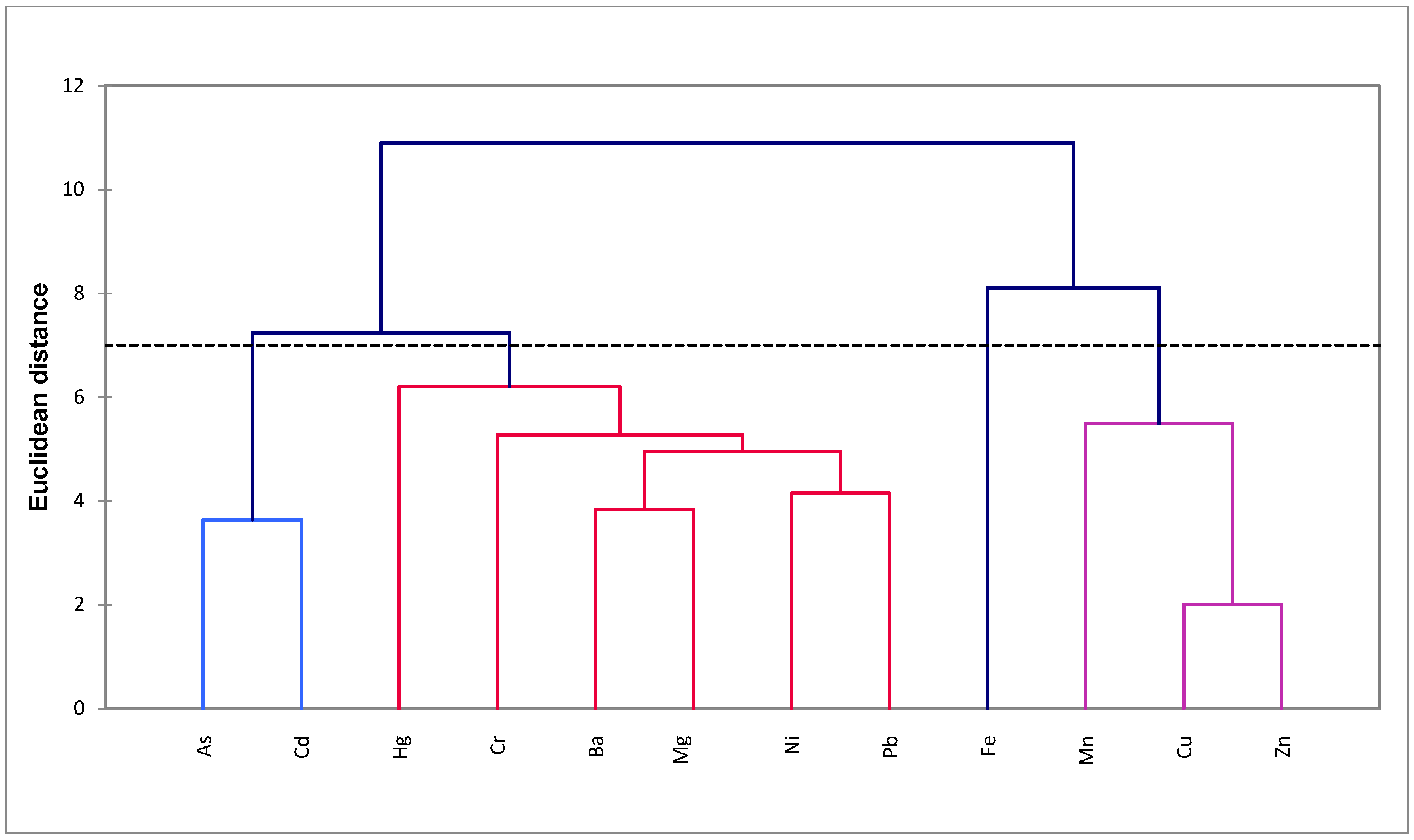
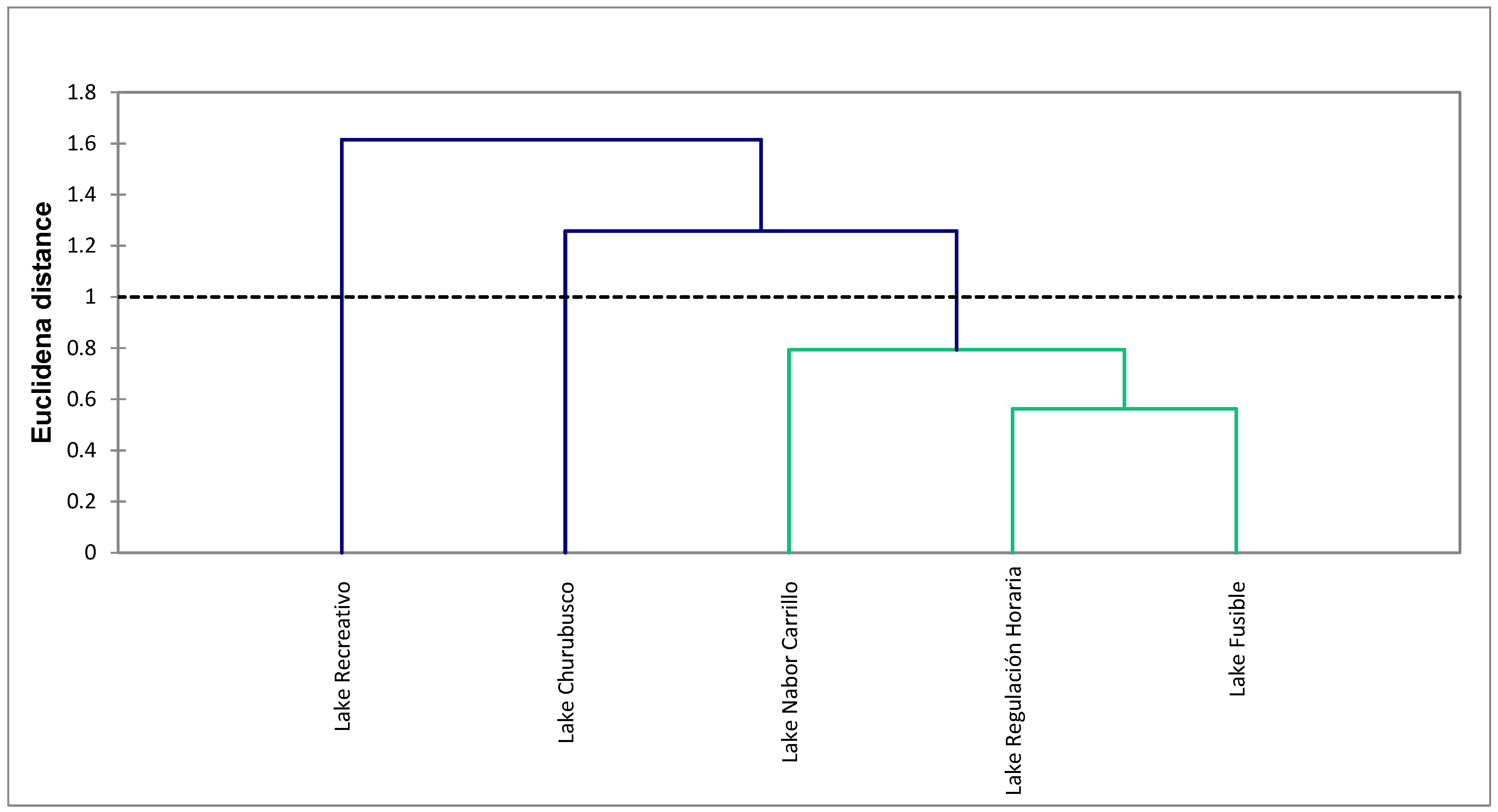
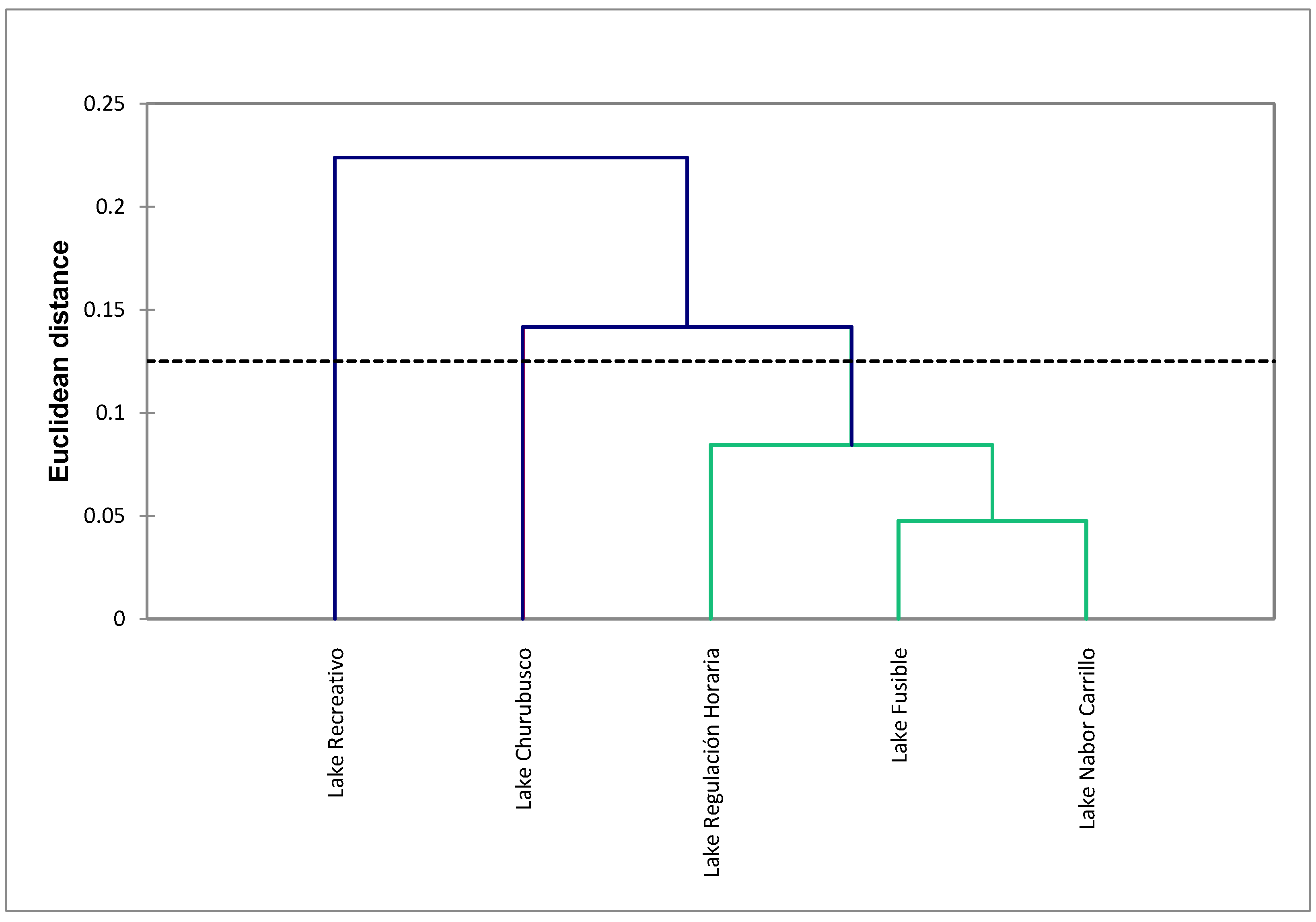
3.4. ANOVA and Hierarchical Cluster Analysis

Significant differences were found for Log(K_d) values of metals in water bodies (one-way ANOVA F = 29.406, p < 0.0001). The Tukey’s multiple comparison test indicates that Log(K_{d Fe}) differs from all other Log(K_d) values. The Hierarchical Cluster Analysis yielded four groups: (I) As and Cd, (II) Hg, Cr, Ba, Mg, Ni, Pb, (III) Mn, Cu, Zn, and (IV) Fe (which differed from all other groups). The clustering corresponds to the gradient of Log(K_d) values (Figure 6). Group I clusters those metals with the lowest Log(K_d) values, i.e., metals available in the water column, in direct contact with the free-swimming aquatic biota. Group II corresponds to metals whose Log(K_d) has intermediate values lower than 3, which according to [22] are also elements prevailing in the liquid phase. Group III includes metals with the highest values, contained mainly in sediments, reflecting the nature of the substrate. Last, Group IV includes only Log(K_{d Fe}), with values suggesting that Fe is associated with the solid phase or particulate materials, forming stable compounds.

The hierarchical cluster analysis by water body shows the similarity between water bodies based on Log (K_d) values; three groups are formed (Figure 7): (I) Recreativo, (II) Churubusco, and (III) Nabor Carrillo, Regulación Horaria, and Fusible. The water body with the greatest dissimilarity is Recreativo, showing the highest MPI values in both water and sediments (Figure 2 and Figure 3), as well as the lowest Log (K_d) values for As and Cd.

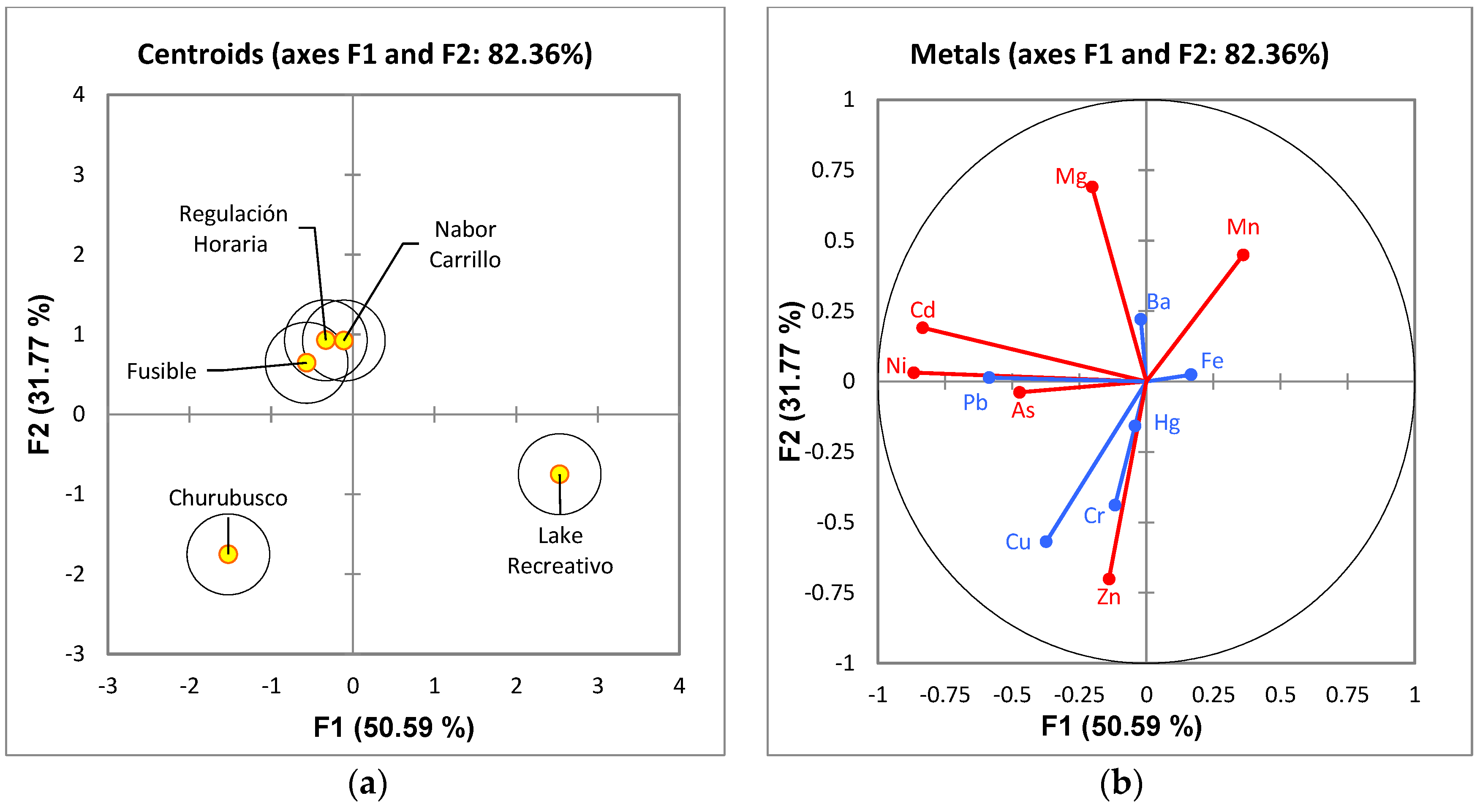
3.5. Discriminant Analysis

A discriminant analysis applied to Log(K_d) values by water body was significant (Wilks Lambda = 0.089, p < 0.0001), with the first two discriminant functions accounting for 82.36% of the explained variance. Centroids represent lakes, and three groups emerge: (I) Recreativo, (II) Churubusco, and (III) Nabor Carrillo, Regulación Horaria, and Fusible. Group I is characterized by the highest Fe and Mn values and the lowest Cd, As, Ni, and Pb, consistent with Figure 4e–g. Group II is characterized by Zn, Cr, and Cu; and Group III is influenced by Cd, Ni, As, and Pb (Figure 8b). All three groups are in agreement with the hierarchical cluster analysis (Figure 7).

3.6. Mean Distribution Coefficient: Ratio MPI_S/MPI_W as a New Index.

The Metal Pollution Index by water body, either in water or sediments (Figure 3 and Figure 4), indicates the average concentration of metals in each water body. MPI_S/MPI_W is the ratio of geometric mean concentrations of metals in sediments and water, corresponding to the mean distribution coefficient of the total metals quantified by water body.

Based on the above, the Mean Distribution Coefficient Index is proposed as:

$${\mathrm{K}}_{\mathrm{d}}{}_{\mathrm{MPI}}=\frac{{\mathrm{MPI}}_{\mathrm{S}}}{{\mathrm{MPI}}_{\mathrm{W}}}$$

(3)

where K_dMPI = Mean Distribution Coefficient based on MPI values calculated for water and sediments.

MPI_S = Metal Pollution Index for metals in sediments.

MPI_W = Metal Pollution Index for metals in water.

Thus, the criteria of Nebelkova and Kominkova [22] can be applied to K_{d MPI} as follows: Log(K_{d MPI}) < 3 indicates that the set of metals is found primarily in the water column. Values of 3 < Log(K_{d MPI}) < 4 include metals released from the solid or particulate phase into the water column. Log(K_{d MPI}) > 5 indicates metals associated with the solid phase. Log(K_dMPI) can be calculated by water body to identify the phase where the set of metals quantified predominates (Figure 9). In the case of the Texcoco artificial lakes, Log (K_{d MPI}) values indicate that Recreativo and Regulación Horaria contain metals mainly in the water column, while Fusible, Nabor Carrillo, and Churubusco have metals in the liquid phase mostly coming from sediments.

A hierarchical cluster analysis applied to the values of the Log(K_{d MPI}) by water body showed three groups (Figure 10): (I) Lake Recreativo, (II) Lake Churubusco, and (III) lakes Nabor Carrillo, Fusible, and Regulación Horaria. This cluster corresponds to the one obtained when Log(K_d) values were used by metal and water body (Figure 7); this clustering is consistent with the Discriminant Analysis.

4. Discussion

4.1. Comparison of Metal Concentrations

Recreativo is the water body that shows the highest mean concentration of Ba, Cd, Cr, Cu, Mg, Hg, Ni, Pb and Zn, in water, and of Ba, Fe, and Mn, in sediments. On the other hand, Nabor Carrillo shows the lowest concentration for most metals.

Metal concentrations in the water bodies of the Lake of Texcoco system fall within the same range of values reported for other shallow saline lakes; however, Ba, Cd, Hg, Ni, and Pb show higher mean values relative to other water bodies. Particularly, Hg shows higher values in both water and sediments.

4.2. Metal Pollution Index

MPI_W and MPI_S results showed a gradient of mean metal content in the Texcoco artificial lakes. In both cases (water and sediments), Recreativo showed the highest MPI values. According to [26], Recreativo and Churubusco were built to increase water storage capacity in the municipality of Texcoco; however, Churubusco currently receives wastewater from México City, while Recreativo is occasionally refilled with groundwater from an area with Solonchak soil. On the other hand, Nabor Carrillo and Regulación Horaria have the lowest MPI_W and MPI_S values, respectively. In this case, MPI values indicate that Recreativo has the highest metal enrichment, with an evident influence of the Solonchak soil. Several authors have used the MPI to compare mean metal concentration in water, sediments, and even in aquatic organisms [51]. Dadolahi and Nazarizadeh [52] found a gradient of metal content based on MPI values in sediments of the coastline of the Hormuzgan province, Iran, ranging from 5 to 10. Adeniyi et al. [53] used the MPI to compare the mean metal concentration along a sampling cycle in the Ebute Ogbo river, finding an inverse correlation of MPI between water and sediments in two consecutive years. As mentioned above, the MPI is an ideal index to compare mean metal concentrations in a region, across water bodies, or in a given water body at different times.

4.3. Distribution Coefficient

Log(K_{d Fe}) values indicate that Fe is highly stable in sediments (solid or particulate phase); on the other hand, Log(K_d) for As and Cd indicates that these metals are contained primarily in the liquid phase, and thus, in direct contact with free-swimming organisms, potentially affecting them [54].

Barreto et al. [16] indicate that less than 200 studies in the literature report K_d values for natural aquatic environments, located mostly in the northern hemisphere. Li et al. [55] estimated the distribution coefficients of five metals in three temperate lakes of China collapsed by mining operations (Cd, As, Pb, Zn, and Sb). Mean Log(K_d) values for Cd, As, Pb, and Zn in the three lakes were 2.56, 3.83, 4.26, and 3.76, respectively. Log (K_{d Cd}) and Log (K_{d Zn}) values in our study were 2.10 and 3.47, respectively; these are closely similar to those obtained by [55], suggesting that the water bodies studied by them have a higher risk of Cd pollution.

Barreto et al. [16] determined the distribution coefficients in the Capivara reservoir in Brazil, a tropical water body. These authors worked with Cd, Cr, Cu, Fe, Mg, Mn, Ni, Pb, and Zn, obtaining the following Log(K_d) values: 3.80, 6.98, 5.86, 6.2, 3.81, 6.37 5.6, 5.49, and 5.84, respectively, which indicate that Cr, Cu, Fe, Mn, Ni, Pb, and Zn are associated mostly with the solid phase. In the present study, the values for the Texcoco lakes show a greater affinity for the liquid phase, with Fe as the metal that comes closest to being in the solid phase.

In a study carried out by the Environmental Protection Agency [56], average Log(K_d) values were obtained for different metals in various freshwater bodies: As (2.5), Ba (4.0), Cd (3.6), Cr (4.5), Cu (4.2), Hg (4.9), Ni (4.0), Pb (5.1), and Zn (3.7). Log(K_d) values for the Texcoco water bodies were lower than those reported by [56]. The lowest value reported by [57] corresponds to As (2.5), while for the Texcoco lakes, Log(K_{d As}) is 2.19, 12.3% lower versus the [57] study. In the Texcoco water bodies, Cd showed the lowest value (2.096), while [56] reported a Log(K_d) value of 3.6 for Cd. For Pb, the Texcoco water bodies showed a Log(K_{d Pb}) of 2.71, while [56] reported a value of 5.1. On the other hand, [16] reported that Log(K_d d) values for Cr, Cu, Ni, and Zn in Lake Capivara were higher than those calculated by [56]. Despite lakes Capivara and Texcoco being tropical water bodies, the latter is influenced by a Solonchak soil. Therefore, the differences recorded may be due to the salinity of the Texcoco water bodies, since some authors report that K_d decreases with salinity [21,57,58,59].

Forghani et al. [14] conducted a study on metal content in Lake Maharlu, a saline continental water body. They found the following gradient: Fe > Mn > Pb > Ni > Cr > Cu > Co > Zn > Cd in terms of absolute concentration of these metals in sediments. Our results in terms of K_d showed the following gradient: Fe > Mn > Zn > Cu > Mg > Cr > Ni > Ba > Pb > Hg > As > Cd, with Fe and Mn as the most abundant metals, and Cd with the lowest K_d value.

The gradient found in the Texcoco water bodies based on Log(K_d) by metal indicates sediments enriched with Fe, Mn, and Zn, typical of Solonchak soils [28], likely forming stable compounds, in agreement with [16]. Likewise, [28,59] determined the concentrations of several metals in Solonchak soil, indicating that Fe and Mn are abundant in this soil type. The stability of certain metals (Log(K_d) > 4) can pose a threat to bottom-dwelling organisms; under certain conditions, these metals could be released to the overlaying water. Metals are generally contained in the liquid phase, and given their toxicity profile, may endanger the whole aquatic ecosystem, as indicated by [55].

4.4. Mean Distribution Coefficient

In this research, a novel index named the Mean Distribution Coefficient herein, is proposed to obtain information about the partitioning of mean metal content in a water body. Log(K_{d MPI}) integrates the information on all metals combined, leading a characterization of a water body (Figure 10) that is similar the one obtained when values for individual metals are used (Figure 7); both approaches ultimately lead to the same three clusters of water bodies. Log(K_{d MPI}) is calculated by water body and not by metal, thus giving an overview of the predominant distribution of metals in the water body and the phase where they prevail.

Based on our results in terms of Log(K_{d MPI}) and considering the criteria of [22], the set of metals studied are being released primarily from sediments into the water column, and highlight the nature of the substrate. When metals are in the liquid phase, they are in contact with the benthic fauna and free-swimming organisms such as fish and macroinvertebrates. The different respiratory systems in these organisms, including the skin, gills, and other specialized respiratory modes, such as accessory pigments, where hemoglobin transports oxygen to the whole organism [60], are also involved in the uptake of metals from the liquid phase [54,61]. This is important for risk assessment studies.

The water bodies of the Lake of Texcoco System are home to a resident community of water birds; additionally, these also host an even larger community of migratory birds during the winter. The detection of the phase where the highest concentration of metals is found and its overall level can be useful in the environmental risk assessment for the bird community (including both migratory and resident species), considering their various food habits. In this case, the Mean Distribution Coefficient may play a central role.

Since some lakes are receptors of both raw and treated wastewater, monitoring the total metal content and the phase where it is found is key. Thus, spatial and temporal variations of the Mean Distribution Coefficient will detect extraordinary metal loads.

Reporting metal levels in terms of the Mean Distribution Coefficient can facilitate summarizing environmental monitoring reports; thus, this is a potentially useful tool for communicating results to society and decision makers.

5. Concluding Remarks

This study provides information about metal pollution in the water bodies of the former Lake of Texcoco, an important continental saline lake of Mexico. MPI is a valuable tool for assessing pollution by metals and facilitates spatial comparisons among water bodies. MPI showed a gradient of metal content in the five lakes studied, where Recreativo was the water body with the highest MPI values, both in water and sediments, while Nabor Carrillo and Regulación Horaria exhibited the lowest concentrations of metals in water and sediments, respectively.

The distribution coefficient reveals the potential mobilization of metals between the liquid and solid phases. Cd and As are the most available elements in the liquid phase in the Texcoco water bodies, and their Log(K_d) values show that, given their toxic properties, these metals may pose a threat to the free-swimming aquatic biota.

The results of the index proposed herein, named Mean Distribution Coefficient K_{d MPI}, were consistent with the results of the Hierarchical Cluster Analysis when applied by water body, using Log(K_d) values for all metals.

The Mean Distribution Coefficient can be a useful tool in assessing ecological risk by metal pollution and in global water quality assessments. This novel index combines the benefits of integrating average concentrations of the metals of interest (through MPI) and the phase where they are mostly located, whether liquid or solid, thus reflecting the migrating capacity of a set of metals between these phases.

References

1. Tang, W.; Shan, B.; Zhang, W.; Zhang, H.; Wang, L.; Ding, Y. Metal pollution characteristics of surface sediments in different aquatic ecosystems in Eastern China: A Comprehensive understanding. PLoS ONE 2014, 9, 1–7. [Google Scholar] [CrossRef]
2. Al-Obaidy, A.H.M.J.; Al-Janabi, Z.Z.; Al-Mashhady, A.A.M. Distribution of some metals in sediments and water in Tigris River. J. Global Ecol. Environ. 2016, 4, 140–146. [Google Scholar]
3. Fernández-Buces, N.; Siebe, C.; Cram, S.; Palacio, J.L. Mapping soil salinity using a combined spectral response index for bare soil and vegetation: A case study in the former lake Texcoco, Mexico. J. Arid Environ. 2006, 65, 644–667. [Google Scholar] [CrossRef]
4. Alkhatib, E.A.; Grunzke, D.; Chabot, T. Multi-Regression Prediction of Metal Partition Coefficients under Various Physical/Chemical Conditions Design of Experiments As, Cr, Cu, Ni and Zn. Hydrol. Curr. Res. 2016, 7, 1–7. [Google Scholar]
5. Singovszka, E.; Balintova, M.; Demcak, S.; Pavlikova, P. Metal Pollution Indices of Bottom Sediment and Surface Water Affected by Acid Mine Drainage. Metals 2017, 7, 284. [Google Scholar] [CrossRef]
6. Wurtsbaugh, W.A.; Miller, C.; Null, S.E.; DeRose, J.; Wilcock, P.; Hahnenberger, M.; Howe, F.; Moore, J. Decline of the world’s saline lakes. Nat. Geosci. 2017, 10, 816–821. [Google Scholar] [CrossRef]
7. Thorne, R.S.J.; Williams, W.P. The response of benthic macroinvertebrates to pollution in developing countries: A multimetric system of bioassessment. Freshw. Biol. 1997, 37, 671–686. [Google Scholar] [CrossRef]
8. Şener, S.; Davraz, A.; Karagüzel, R. Assessment of trace metal contents in water and bottom sediments from Egirdir Lake, Turkey. Environ. Earth Sci. 2014, 71, 2807–2819. [Google Scholar]
9. Gurung, B.; Kominkova, D.; Race, M.; Fabricino, M. Assessment of toxic metals mobility in water-sediment environment of the Lambro Creek, Italy. In Proceedings of the 15th International Conference on Environmental Science and Technology, Rhodes, Greece, 31 August–2 September 2017; CEST: Athens, Greece, 2017. [Google Scholar]
10. Njenga, J.W.; Ramanathan, A.L.; Subramanian, V. Partitioning of metals in the sediments of Lake Naivasha, Kenya. Chem. Spec. Bioavailab. 2009, 21, 41–48. [Google Scholar] [CrossRef]
11. Rajeshkumar, S.; Liu, Y.; Zhang, X.; Ravikumar, B.; Bai, G.; Li, X. Studies on seasonal pollution of metals in water, sediment, fish and oyster from the Meiliang Bay of Taihu Lake in China. Chemosphere 2018, 191, 626–638. [Google Scholar] [CrossRef]
12. Wu, B.; Wang, G.; Wu, J.; Fu, Q.; Liu, C. Sources of Metals in Surface Sediments and an Ecological Risk Assessment from Two Adjacent Plateau Reservoirs. PLoS ONE 2014, 9, 1–14. [Google Scholar] [CrossRef] [Green Version]
13. Angeler, D.G.; Allen, C.R.; Birgé, H.E.; Drakare, S.; McKie, B.G.; Johnson, R.K. Assessing and managing freshwater ecosystems vulnerable to environmental change. Ambio 2014, 43, 113–125. [Google Scholar] [CrossRef] [Green Version]
14. Forghani, G.; Farid, M.; Afshin, Q. The Concentration and Partitioning of Metals in Surface Sediments of the Maharlu Lake, SW Iran. Soil Sediment Contam. 2012, 21, 872–888. [Google Scholar] [CrossRef]
15. Herojeet, R.; Rishi, M.S.; Kishore, N. Integrated approach of metal pollution indices and complexity quantification using chemometric models in the Sirsa Basin, Nalagarh valley, Himachal Pradesh, India. Chin. J. Geochem. 2015, 34, 620–633. [Google Scholar] [CrossRef]
16. Giancoli Barreto, S.R.; Barreto, W.J.; Deduch, E.M. Determination of partition coefficients of metals in natural tropical water. Clean Soil Air Water 2011, 39, 362–367. [Google Scholar] [CrossRef]
17. Boyer, P.; Wells, C.; Howard, B. Extended Kd distributions for freshwater environment. J. Environ. Radioactiv. 2018, 192, 128–142. [Google Scholar] [CrossRef]
18. Usero, J.; González, E.; Regalado, L.; Gracia, I. Trace Metals in the Bivalve Mollusc Chamelea gallina from the Atlantic Coast of Southern Spain. Baseline 1996, 32, 305–310. [Google Scholar] [CrossRef]
19. Sedeño-Díaz, J.E.; Rodríguez-Romero, A.J.; Mendoza-Martínez, E.; López-López, E. Chemometric Analysis of Wetlands Remnants of the Former Texcoco Lake: A Multivariate Approach. In Lake Sciences and Climate Change, 1st ed.; Mohamed, N.R., Ed.; Intech Open: Rijeca, Croatia, 2016; Volume 8, pp. 135–153. [Google Scholar]
20. Takata, H.; Keiko, T.; Tatsuo, A.; Shigeo, U. Distribution coefficients (Kd) of strontium and significance of oxides and organic matter in controlling its partitioning in coastal regions of Japan. Sci. Total Environ. 2014, 490, 979–986. [Google Scholar] [CrossRef]
21. Thanh-Nho, N.; Stardy, E.; Nhu-Trang, T.T.; David, F.; Marchand, C. Trace metals partitioning between particulate and dissolved phases along a tropical mangrove estuary (Can Gio, Vietnam). Chemosphere 2018, 196, 311–322. [Google Scholar] [CrossRef]
22. Nabelkova, J.; Kominkova, D. Trace Metals in the Bed Sediment of Small Urban Streams. Open Environ. Biol. Monit. J. 2012, 5, 48–55. [Google Scholar] [CrossRef] [Green Version]
23. Durrieu, G.; Ciffroy, P.; Garnier, J.M. A weighted bootstrap method for the determination of probability density functions of freshwater distribution coefficients (Kds) of Co, Cs, Sr and I radioisotopes. Chemosphere 2006, 65, 1308–1320. [Google Scholar] [CrossRef]
24. Taher, A.; Soliman, A. Metal concentrations in surficial sediments from Wadi El Natrun saline lakes, Egypt. Inter. J. Salt Lake Res. 1999, 8, 75–92. [Google Scholar] [CrossRef]
25. Forghani, G.; Moore, F.; Lee, S.; Qishlaqi, A. Geochemistry and speciation of metals in sediments of the Maharlu Saline Lake, Shiraz, SW Iran. Environ. Earth Sci. 2009, 59, 173–184. [Google Scholar] [CrossRef]
26. Alcocer, J.; Williams, W.D. Historical and recent changes in Lake Texcoco, a saline lake in Mexico. J. Salt Lake Res. 1996, 5, 45–61. [Google Scholar] [CrossRef]
27. Luna-Guido, M.L.; Beltrán-Hernández, R.I.; Solís-Ceballos, N.A.; Hernández-Chávez, N.; Mercado-García, F.; Catt, J.A.; Olalde-Portugal, V.; Dendooven, L. Chemical and biological characteristics of alkaline saline soils from the former Lake Texcoco as affected by artificial drainage. Biol. Fertil. Soils 2000, 32, 102–108. [Google Scholar] [CrossRef]
28. Navas, A.; Lindhorfer, H. Geochemical speciation of metals in semiarid soils of the central Ebro Valley (Spain). Environ. Inter. 2003, 29, 61–68. [Google Scholar] [CrossRef] [Green Version]
29. Leal, J.A.R.; Medrano, C.N.; Silva, F.T. Aquifer vulnerability and groundwater quality in mega cities: Case of the Mexico Basin. Environ. Earth Sci. 2010, 61, 1309–1320. [Google Scholar] [CrossRef]
30. Arce, J.L.; Layer, P.W.; Macías, J.L.; Morales-Casique, E.; García-Palomo, A.; Jiménez-Domínguez, F.J.; Benowitz, J.; Vásquez-Serrano, A. Geology and stratigraphy of the Mexico Basin (Mexico City), central Trans-Mexican Volcanic Belt. J. Maps 2019, 15, 320–332. [Google Scholar] [CrossRef]
31. Lorenzo, J.L.; Mirambell, L. Tlapacoya: 35000 años de historia del Lago de Chalco. Colección Científica INAH-SEP, Serie Prehistoria; Instituto Nacional de Antropología e Historia: Mexico City, México, 1986; p. 297.
32. Elizondo, R.R. Memoria de las Obras del Sistema de Drenaje Profundo del Distrito Federal; Departamento del Distrito Federal: Ciudad de México, México, 1975. [Google Scholar]
33. Alcantara, J.L.; Escalante, P. Current Threats to the Lake Texcoco Globally Important Bird Area; USDA Forest Service: Washington, DC, USA, 2005.
34. García, E. Modificaciones al Sistema de Clasificación Climática (Para Adaptarlo a las Condiciones de la República Mexicana, 6th ed.; UNAM: Mexico City, Mexico, 2004; p. 90. [Google Scholar]
35. Government of Mexico. Available online: https://www.gob.mx/cms/uploads/attachment/file/166769/NMX-AA-014-1980.pdf (accessed on 18 September 2019).
36. USEPA. Methods for Collection, Storage and Manipulation of Sediments for Chemical and Toxicological Analyses: Technical Manual; EPA-823-B-01-002; United States Environmental Protection Agency: Washington, DC, USA, 2001.
37. Ministry of Economy. Available online: http://www.economia-nmx.gob.mx/normas/nmx/2010/nmx-aa-132-scfi-2016.pdf (accessed on 18 September 2019).
38. Government of Mexico. Available online: https://www.gob.mx/cms/uploads/attachment/file/166150/nmx-aa-115-scfi-2015.pdf (accessed on 18 September 2019).
39. Government of Mexico. Available online: https://www.gob.mx/cms/uploads/attachment/file/ 166788/NMX-AA-072-SCFI-2001.pdf (accessed on 8 December 2019).
40. Government of Mexico. Available online: https://www.gob.mx/cms/uploads/attachment/file/ 166146/nmx-aa-034-scfi-2015.pdf (accessed on 8 December 2019).
41. Navarrete-López, M.; Jonathan, M.P.; Rodríguez-Espinosa, P.F.; Salgado-Galeana, J.A. Autoclave decomposition method for metals in soils and sediments. J. Environ. Monit. Assess. 2012, 184, 2285–2293. [Google Scholar] [CrossRef]
42. Government of Mexico. Available online: https://www.gob.mx/cms/uploads/attachment/file/166785/NMX-AA-051-SCFI-2001.pdf (accessed on 18 September 2019).
43. Martin, T.D.; Brockhoff, C.A.; Creed, J.T. EMMC Methods Work Group—Method 200.7, Revision 4.4: Determination of Metals and Trace Elements in Water and Wastes by Inductively Coupled Plasma-Atomic Emission Spectrometry; Environmental Protection Agency: Cincinnati, OH, USA, 1994; p. 59.
44. SGS-U.S. Geological Survey Office of Water Quality. USGS Water-Quality Information: Water Hardness and Alkalinity. Available online: https://canvas.jmu.edu>files>dowload (accessed on 18 September 2019).
45. Bahnasawy, M.; Khidr, A.A.; Dheina, N. Assessment of heavy metal concentrations in water, plankton, and fish of Lake Manzala, Egypt. Turk. J. Zool. 2011, 35, 271–280. [Google Scholar] [CrossRef] [Green Version]
46. Moore, F.; Forghan, G.; Qishlaq, A. Assessment of heavy metal contamination in water and surface sediments of the Maharlu saline lake, SW Iran. Iran J. Sci. Technol. 2009, 33, 43–55. [Google Scholar]
47. Ochieng, E.Z.; Lalah, J.O.; Wandiga, S.O. Analysis of Heavy Metals in Water and Surface Sediment in Five Rift Valley Lakes in Kenya for Assessment of Recent Increase in Anthropogenic Activities. Bull. Environ. Contam. Toxicol. 2007, 79, 570–576. [Google Scholar] [CrossRef] [PubMed]
48. Liu, H.; Li, W. Dissolved trace elements and heavy metals from the shallow lakes in the middle and lower reaches of the Yangtze River region, China. Environ. Earth Sci. 2011, 62, 1503–1511. [Google Scholar] [CrossRef]
49. Stojanovica, A.; Kogelniga, D.; Mittereggera, B.; Maderb, D.; Jirsaa, F.; Krachlera, R.; Krachler, R. Major and trace element geochemistry of superficial sediments and suspended particulate matter of shallow saline lakes in Eastern Austria. Chem. Erde-Geochem. 2009, 69, 223–234. [Google Scholar] [CrossRef]
50. Bayanmunkh, B.; Sen-Lin, T.; Narangarvuu, D.; Ochirkhuyag, B.; Bolormaa, O. Physico-Chemical Composition of Saline Lakes of the Gobi Desert Region, Western Mongolia. J. Earth Sci. Clim. Chang. 2017, 8, 1–7. [Google Scholar]
51. Obluchinskaya, E.D.; Aleshina, E.G.; Matishov, D.G. Comparative Assessment of the Metal Load in the Bays and Inlets of Murmansk Coast by the Metal Pollution Index. Oceanology 2013, 448, 236–239. [Google Scholar] [CrossRef]
52. Öğlü, B.; Yorulmaz, B.; Genç, T.O.; Yilmaz, F. The Assessment of Metal Content by Using Bioaccumulation Indices in European Chub, Squalius cephalus (Linnaeus, 1758). Carpath. J. Earth Environ. 2015, 10, 85–94. [Google Scholar]
53. Dadolahi, A.S.; Nazarizadeh, M.D. Metals Contamination in Sediments from the North of the Strait of Hormuz. Mar. Sci. 2013, 4, 39–46. [Google Scholar]
54. Adeniyi, A.A.; Owoade, O.J.; Shotonwa, I.O.; Okedeyi, O.O.; Ajibade, A.A.; Sallu, A.R.; Olawore, M.A.; Ope, K.A. Monitoring metals pollution using water and sediments collected from Ebute Ogbo river catchments, Ojo, Lagos, Nigeria. Afr. J. Pure Appl. Chem. 2011, 5, 219–223. [Google Scholar]
55. Li, Y.; Liu, F.; Zhou, X.; Wnag, X.; Liu, Q.; Zhu, P.; Zhang, L.; Sun, C. Distribution and Ecological Risk Assessment of Metals in Sediments in Chinese Collapsed Lakes. Pol. J. Environ. Stud. 2017, 26, 181–188. [Google Scholar] [CrossRef]
56. Allison, J.D.; Allison, T.L. Partition Coefficients for Metals in Surface Water, Soil, and Waste; U.S. Environmental Protection Agency: Washington, DC, USA, 2005; p. 93.
57. Turner, A. Trace-metal partitioning in estuaries: Importance of salinity and particle concentration. Mar. Chem. 1996, 54, 27–39. [Google Scholar] [CrossRef]
58. Baeyens, W.; Parmentier, K.; Goeyens, L.; Ducastel, G.; De Gieter, M.; Leermakers, M. The biogeochemical behaviour of Cd, Cu, Pb and Zn in the Scheldt estuary: Results of the 1995 surveys. Hydribiología 1998, 366, 45–62. [Google Scholar] [CrossRef]
59. Seida, Y. Influence of Salinity and pH of Solution on Partition Coefficient of Ion at Solution—Charged Media Interface. J. Toyo Univ. Nat. Sci. 2014, 58, 57–66. [Google Scholar]
60. Navas, A.; Machín, J. Spatial distribution of metals and arsenic in soils of Aragón (northeast Spain): Controlling factors and environmental implications. Appl. Geochem. 2002, 17, 961–973. [Google Scholar] [CrossRef] [Green Version]
61. Jesus, T. Ecological, anatomical and physiological traits of benthic macroinvertebrates: Their use on the health characterization of freshwater ecosystems. Limnetica 2008, 27, 79–92. [Google Scholar]
Figure 1. Study area. Geographic location of the study area (a), topographic map of the surrounding area of the Lake of Texcoco System (b), and map of soil types showing the location of lakes (c).
Water 12 00029 g001
Figure 2. Box and whisker plot of MPIW by water body.
Water 12 00029 g002
Figure 3. Box and whisker plot of MPI by water body.
Water 12 00029 g003
Figure 4. Box and whisker plot of Log(Kd) by metal and water body: (a) Fe, (b) Mn, (c) Zn, (d) Cu, (e) Mg, (f) Cr, (g) Ni, (h) Ba, (i) Pb, (j) Hg, (k) As, and (l) Cd.
Water 12 00029 g004
Figure 5. Box and whisker plot of mean Log(Kd) for the studied metals considering all water bodies. The blue band includes Log(Kd) < 3; the orange band, 3 < Log(Kd) < 4; and the white band, Log(Kd) > 4, as indicated by the criteria of Nebelkova and Kominkova [22].
Water 12 00029 g005
Figure 6. Dendrogram showing clustering by Log(Kd) values of each metal.
Water 12 00029 g006
Figure 7. Dendrogram showing the clustering of water bodies based on Log(Kd) values.
Water 12 00029 g007
Figure 8. Biplot of Discriminant Analysis of Log(Kd) values by metal and water body. (a) Study sites; (b) Vectors of metals.
Water 12 00029 g008
Figure 9. Box and whisker plot of Log(Kd MPI) for all water bodies.
Water 12 00029 g009
Figure 10. Dendrogram showing the clustering of Mean Distribution Coefficients across water bodies.
Water 12 00029 g010