An Analysis of Energy Consumption and the Use of Renewables for a Small Drinking Water Treatment Plant

Abstract

One of the pressing issues currently faced by the water industry is incorporating sustainability considerations into design practice and reducing the carbon emissions of energy-intensive processes. Water treatment, an indispensable step for safeguarding public health, is an energy-intensive process. The purpose of this study was to analyze the energy consumption of an existing drinking water treatment plant (DWTP), then conduct a modeling study for using photovoltaics (PVs) to offset that energy consumption, and thus reduce emissions. The selected plant, located in southwestern United States, treats 0.425 m³ of groundwater per second by utilizing the processes of coagulation, filtration, and disinfection. Based on the energy consumption individually determined for each unit process (validated using the DWTP’s data), the DWTP was sized for PVs (as a modeling study). The results showed that the dependency of a DWTP on the traditional electric grid could be greatly reduced by the use of PVs. The largest consumption of energy was associated with the pumping operations, corresponding to 150.6 Wh m⁻³ for the booster pumps to covey water to the storage tanks, while the energy intensity of the water treatment units was found to be 3.1 Wh m⁻³. A PV system with a 1.5 MW capacity with battery storage (30 MWh) was found to have a positive net present value and a levelized cost of electricity of 3.1 cents kWh⁻¹. A net reduction in the carbon emissions was found as 950 and 570 metric tons of CO₂-eq year⁻¹ due to the PV-based design, with and without battery storage, respectively.

1. Introduction

Recently, there has been an increased emphasis on including sustainability into water infrastructure design and reducing the carbon emissions of water-related processes [1,2]. One way to achieve these goals is to incorporate renewables into the operation of water and wastewater treatment plants in order to offset their energy consumption. Solar energy, particularly through photovoltaic conversion, is a promising way to meet the world’s future energy demands. Solar energy helps reduce dependence on fossil fuel-based energy sources, as well as reduce environmental pollution, including carbon emissions, caused by fossil fuel use [3,4,5]. In this study, the energy consumption of a small drinking water treatment plant (DWTP) was analyzed; then, a techno-economic assessment for using solar photovoltaics (PVs) was conducted to offset that energy consumption and reduce carbon emissions.

Water treatment is an integral component of modern life, and is vital for safeguarding the health of any community. In the United States, there are about 60,000 small and large DWTPs, and about 15,000 wastewater treatment facilities, which consume about 3%–4% of the overall energy [6]. The energy consumption of drinking water and wastewater treatment plants (WWTPs) has been evaluated by various studies [7,8,9,10,11,12]. Ref. [8,9] determined the energy consumption and the associated carbon emissions for water reuse plants and WWTPs, respectively, whereas [11] utilized metafrontier data envelopment analysis to analyze the energy efficiency of DWTPs. Ref. [12] reported that the city of Qingdao, China, utilized about 1% of its total energy consumption for drinking water treatment, whereas utilization was 4%–5% for the distribution of the drinking water, as well as the treatment of the generated wastewater.

The changing climate, coupled with the growing population, places increased demands on water treatment facilities [13]. Between the years 1950–2000, the United States’ population increased from 152.3 to 272.7 million [14], but the demands on its water supply systems increased by more than three-fold during this period, as determined by the U.S. Environmental Protection Agency (USEPA) [15]. The energy consumption of DWTPs and WWTPs corresponds to about 56–75 billion kWh year⁻¹ [16,17], and costs about $4 billion annually [6]. These facilities account for up to 35% of a municipal government’s energy budget [18]. A reduction in carbon emissions and reduced energy costs may be the motivating factors for incorporating PVs into the design of existing water infrastructures [15]. Ref. [19] determined that among the 105 WWTPs operating in California treating about 78% of the wastewater of the state, 41 WWTPs utilized solar PVs to offset their energy consumption, most which are located in rural settings.

However, solar energy deployment faces barriers related to land resource availability and financial constraints [20]. Solar installations require large land resources; therefore, the development of solar energy may be limited because of land constraints, especially in urban areas. Proximity to military bases, airports, and high population density zones also prevent the use of PVs [21]. As smaller DWTPs are typically present in smaller, more remote communities, which are likely to have land available, the application of PVs has the potential to increase the sustainability of such plants. The implementation of solar energy may also be limited because of economic constraints. Financial barriers include high capital costs, taxes, and costs associated with storage [22,23].

Various tools exist to model the technical and economic performance of PV systems. The Solar Deployment System (SolarDS) model has been developed by the National Renewable Energy Laboratory (NREL) [24], which simulates the performance of PV technology on building rooftops in the United States until 2030. The Solar and Wind Energy Resource Assessment (SWERA) is a freely available tool [25] that provides international resource data sets and analysis tools related to solar and wind energy in a dynamic user-friendly setting. The System Advisor Model (SAM), utilized for the current study, is a techno-economic modeling tool, developed by the U.S. Department of Energy and NREL [26,27]. Various studies have used SAM for analyzing solar technologies [28,29,30,31,32]. Ref. [28] analyzed a 86 kW commercial PV system using SAM, and found it to achieve grid parity. Ref. [29] analyzed the effect of shading on 46 residential PV systems, and compared the on-site performance measurements with the performance estimations generated by SAM. The comparison showed the median yearly bias errors to be less than or equal to 2.5%, determining SAM to be a reliable model for shading analysis. Ref. [30] reviewed various renewable energy simulation models, including SAM. Ref. [31] conducted techno-economic assessments for three DWTPs using SAM.

The southwestern United States possesses tremendous solar resources, and is a prime candidate for PV implementation [33,34]. Water and wastewater treatment facilities located in areas of high solar intensity can achieve sustainability by incorporating PVs into their energy source portfolio [35,36,37,38,39]. Few studies have explored the incorporation of solar energy for DWTPs [39,40,41,42]. Ref. [39] performed a techno-economic analysis using solar (5.6 MW) and wind energy (8 MW), coupled with and without battery storage to meet 96% and 88% of the energy demand of a water treatment plant treating 3.11 m³ of water per second, respectively. Ref. [40,41] evaluated the performance of PVs for small communities in the United States and in Pakistan, respectively. Ref. [42] analyzed the performance of 16 small-scale solar-powered existing DWTPs located in rural settings without electricity access, across Egypt’s Western Desert, which primarily treated groundwater for iron removal (exceeding the World Health Organization’s standard of 0.3 mg L⁻¹).

The objectives of the current investigation were as follows:

• Design a DWTP to compute the energy requirements for the plant operation by focusing on the energy driving units of each treatment process and validating it using the plant’s data;
• Conduct a modeling study for using PV to meet the energy requirements of the plant;
• Compare the existing land-holdings of the plant with the land requirement for the proposed PV system;
• Evaluate the economics of using solar PV;
• Determine the reduction in carbon emissions compared with non-PV based design.

2. Study Area

The selected DWTP provides treated groundwater to a city with a population of less than 10,000. The plant has the capacity to treat 0.425 m³ of water per second, and is located in the southwestern region of the United States, where the solar intensity is highly favorable for PV generation. The actual location of the plant cannot be disclosed because of confidentiality. For analysis purposes, it was assumed that the plant was located in rural Nevada (annual direct beam insolation of 6.8 kWh m⁻² day⁻¹). The raw water is contaminated by one element, arsenate As (V), with levels of around 100 ppb. This value exceeds the USEPA’s limit of 10 ppb, set as the maximum contaminant level for arsenic in public water supplies. The DWTP is considered a small system under the Safe Drinking Water Act, as it serves a community of 10,000 or less [43]. The plant operates 24 hours per day, and is 12 years old.

3. Data Sources

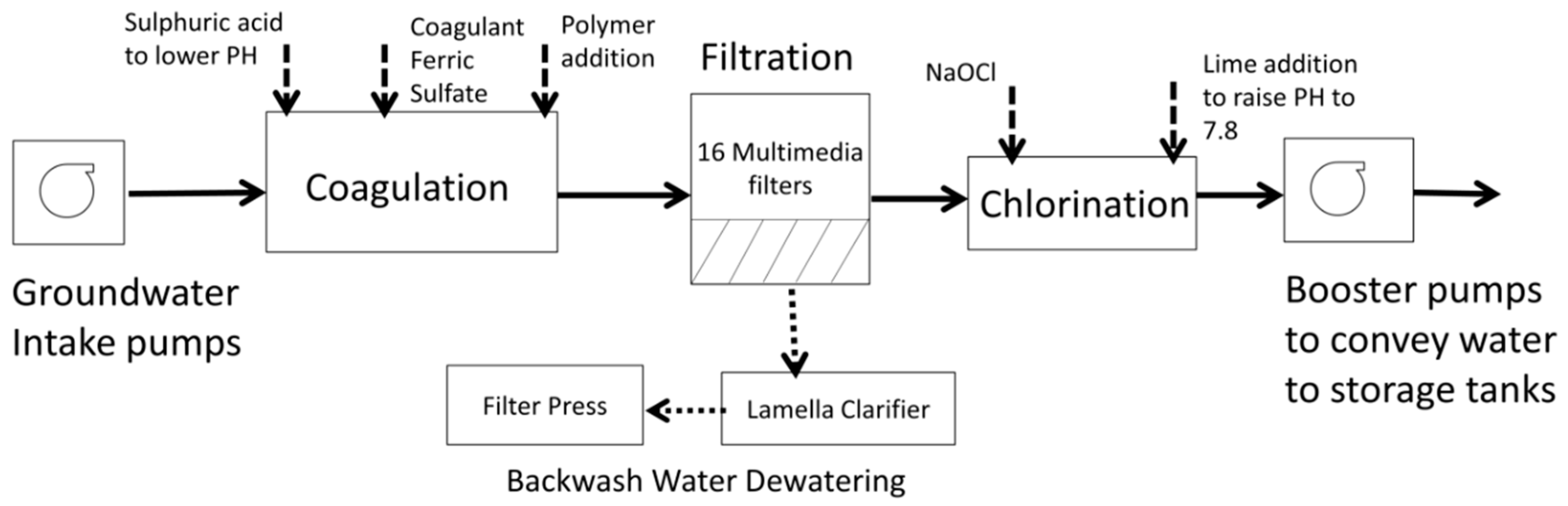
The data used in this study consist of a raw water quality report (

Table 1. Water quality characteristics for the treatment plant.

Parameter	Unit	Average Value	U.S. Environmental Protection Agency (USEPA) MCL */SMCL **/Guidelines
pH	-	8	6.5–8.5
Water temperature	°C	19	Not regulated
Arsenic	mg L−1	100	10

* MCL: Maximum contaminant level. ** SMCL: Secondary maximum contaminant level.

), a process flow diagram (Figure 1) of the DWTP and plant’s operational details obtained from the DWTP managers. Additional data to design the unit operations was obtained from [44]. The raw groundwater displays the characteristics of low turbidity <5 NTU, low TOC <4 mg L⁻¹, and low color <10 c.u. The treatment train consists of coagulation, followed by filtration, and disinfection (Figure 1).

The data used to estimate the net reduction carbon emissions were obtained from [45]. Ref. [45] provided median estimates of the carbon emission data in units of gCO₂eq kWh⁻¹ as 4 for hydroelectric energy, 12 for wind energy, 16 for nuclear energy, 18 for energy generated from biomass, 45 for geothermal energy, 46 for photovoltaics, 469 for natural gas, 840 for petroleum-based energy, and 1001 for coal generated energy. The sources of electricity, also known as the electricity mix or energy mix, for Nevada, were obtained from the U.S. Energy Information Administration (USEIA) [46] as shown in

Table 2. Nevada’s electricity source mix for various energy sources.

Energy Sources for Electricity Generation	State Electricity Source Mix (%)
Coal	23.51
Natural gas	56.41
Petroleum	0.07
Bio-power	0.1
Geothermal	8.5
Hydropower	7.42
Nuclear	0
Solar	3.04
Wind	0.95

.

The financial parameters used to perform the economic evaluation were based on the review of literature published in the years of 2016 and 2017 [22,23,47,48,49,50,51,52,53,54,55,56,57,58,59] (

Table 3. Financial parameters used for economical assessment using the System Advisor Model (SAM).

System Cost Components	Parameter	Unit	Values	References
Direct Cost	Module	$ Watt−1	0.87	[48]
	Inverter	$ Watt−1	0.29	[47]
	Battery bank	$ kWh−1	160	[49]
	Electrical Balance of equipment cost	$ Watt−1	0.16	[50]
	Fixed tilt Racking	$ Watt−1	0.10	[50]
	One−axis tracking equipment	$ Watt−1	0.15	[50,51]
	Two-axis-tracking equipment	$ Watt−1	0.20	[52]
	Installation labor	$ Watt−1	0.13	[50]
	Contingency	%	4.0	[50]
Indirect Capital Cost	Permitting, environmental studies, and grid interconnection	$ Watt−1	0.10	[50]
	Engineering and developer overhead	$ Watt−1	0.57	[50]
O&M * cost Debt	Fixed annual cost	$ kW−1 year−1	$15	[50]
	Debt fraction	%	100	-
	Loan term	Years	25	[53,54]
	Loan rate	% year−1	3.0	[55]
	Inflation rate	%	2.5	SAM default value
	Real discount rate	%	8.0	[22,23]
Tax, insurance, discount rates	Federal income tax rate	% year−1	28	[22]
	State income tax rate	% year−1	0.0	[56]
	Sales tax	%	8.1	[56]
	Insurance rate Salvage value	% of installed costs	0.25 20	[57] [58]
	Property tax rate	% year−1	0.0	[59]
Battery	Battery bank replacement cost	$ kWh−1	110	[39]

* O&M cost-operation and maintenance cost.

). Module and inverter types for the design of the PV system were selected from the SAM database; their parameters were used to design the number of modules and inverters, as well as the system capacity. The selected PV system characteristics and costs were found in the literature [47,48,49] and incorporated into SAM for the techno-economic analysis (

Table 4. Photovoltaic system design characteristics used in SAM.

PV System Components	Parameter	Unit	Value
Module	Module name	-	Centrosolar America BP6-260BB
	Module area	m²	1.637
	Module material	-	Multi-crystalline silicon
	Nominal efficiency	%	15.9
	Maximum power (Pmp)	Watt	260
	Maximum power voltage (Vmp)	Volt	31.1
	Maximum power current (Imp)	Ampere	8.4
	Open circuit voltage (Voc)	Volt	37.8
	Short circuit voltage (Isc)	Ampere	8.9
Inverter	Inverter name	-	Sunpower: SPR-4000
	Weighted efficiency	%	95.4
	Maximum AC power	Watt	4000
	Maximum DC power	Watt	4198
	Nominal AC voltage	Volt	240
	Maximum DC voltage	Volt	480
	Maximum DC Current	Ampere	0.008
	Minimum MPPT * DC voltage	Volt	100
	Nominal DC voltage	Volt	300
	Maximum MPPT DC voltage	Volt	480
Battery Storage	Battery name	-	Lead acid AGM **
	Cell nominal voltage	Volt	2
	Internal resistance	m Ohm	2
	Cell capacity	Ah	1200
	Minimum state of charge	%	10
	Maximum state of charge	%	95
	Minimum time at charge state	min	10
	25% Depth of discharge cycle	-	2500
	50% Depth of discharge cycle	-	1250
	75% Depth of discharge cycle	-	650

* Maximum Power Point Tracking. ** Absorbent glass mat.

). A multi-crystalline silicone module was used because it is more efficient compared to other types of panels. Sunpower SPR-4000 [47] was the grid-tied interactive inverter utilized for this study. The battery storage that was selected was a lead acid absorbent glass mat (AGM) 1200-Ah battery.

4. Methodology

The unit processes of the DWTP were designed using the data provided by the DWTP managers. The design of the plant and the estimation of the energy consumption were determined for the maximum flow anticipated for the design life of the plant (36.72 × 10³ m³ day⁻¹) for the DWTP. Thus, the analysis was representative of the worst-case scenario for the DWTP. The other parameters chosen were also reflective of the extreme conditions. The components of the unit processes governing the energy usage were identified and the energy consumption was determined (Section 4.1); these estimates were then validated by comparing the estimated motor sizes with the plant’s motor sizes. To offset the energy consumption of the DWTP, a techno-economic assessment of the proposed PV system was modeled using SAM (Section 4.2). The details are as follows.

4.1. Energy Consumption

The selected DWTP treated groundwater obtained from seven wells, located at a distance of about 10 km from the treatment plant. The coagulation and filtration steps of the DWTP aimed to reduce the arsenic levels from 100 to 10 ppb (Figure 1). Chlorination was used for disinfection, and for the chlorine residual to travel through the distribution system. Booster pumps were used to pump the water to elevated storage tanks.

The water entered the treatment plant and underwent a coagulation process. The mixing of ferric sulfate (coagulant) with water for the formation of flocs occurred in the conduit structure between the coagulation and filtration processes. Metering pumps were used for the coagulant addition, sulfuric acid (pH reduction), and polymer addition (flocculation aid). The energy consumption associated with the pumping operation was determined using criteria provided by the Water Environment Federation [60]. The criterion provided by [61] was used to design the multi-media filters for the separation of the flocs from the liquid. Anthracite, sand, and garnet made up the media composition of the multimedia-filter, with layer depths of 530, 230, and 115 mm, respectively. Surface wash pumps, used to break up the clogged surface layer of the filter media, were designed based on the criteria provided by [62]. The multi-media filter was backwashed once per day. The wash water, generated after backwashing, flowed by gravity, and was stored in a tank before being pumped into a lamella clarifier for treatment. The filters were backwashed to avoid the bio fouling of the filters, based on either a pre-defined schedule or when the head loss exceeded the available operating head (1.8–3 m). Next, sodium hypochlorite was used for disinfection.

Chlorination was designed using the criteria provided by [44,63]. Based on the USEPA groundwater rule, the groundwater was chlorinated for the four-log removal of viruses and for achieving a chlorine residual in the distribution system. For effective mixing, the chlorine contact tank was equipped with baffles, based on the design criteria provided by [63]. A CT (product of contact time and concentration of free chlorine residual) value of 12 mg L⁻¹ min was used for the design of the chlorine contact basins. After the water was chlorinated, lime slurry was added to increase the pH to 7.8. The lime was delivered in bulk form and was mixed on site. The energy consumption related to the mixing operation was estimated based on the criteria provided by [61]. The daily lime requirements were 3.2 m³ day⁻¹. The energy consumption of the lime slurry addition to the finished water, using a metering pump, was determined using the criteria provided by [60]. Booster pumps were used to transport the treated water from the treatment plant to an elevated storage tank to be further distributed throughout the city.

For the treatment of the backwash water generated in the filters, a lamella clarifier and filter press were used. The lamella clarifier was an improvement over the conventional sedimentation process, as the area requirements were reduced by almost 90%, compared with the latter case. The lamella clarifier was designed using the criteria provided by [62]. The solids accumulated and then slid off the inclined plates (at 45° angle) under gravity. The waste sludge obtained from the operation of the lamella clarifier was dewatered using a belt-filter press. This mechanical dewatering technique involved moving belts for the continuous dewatering of sludge through the application of a gravity drainage zone (water is removed from the sludge under gravity on a conveying belt) and a pressure zone (the sludge was sandwiched between the upper and lower belts, while the contact pressure increased from low to high). The end-products were filtrate and sludge cake with 20%–30% solids. The design and energy consumption estimation associated with the belt-filters was based on the criteria provided by [64]. The tables and figures showing the results for the application of this methodology are discussed later in Section 5.1.

4.2. System Advisor Model

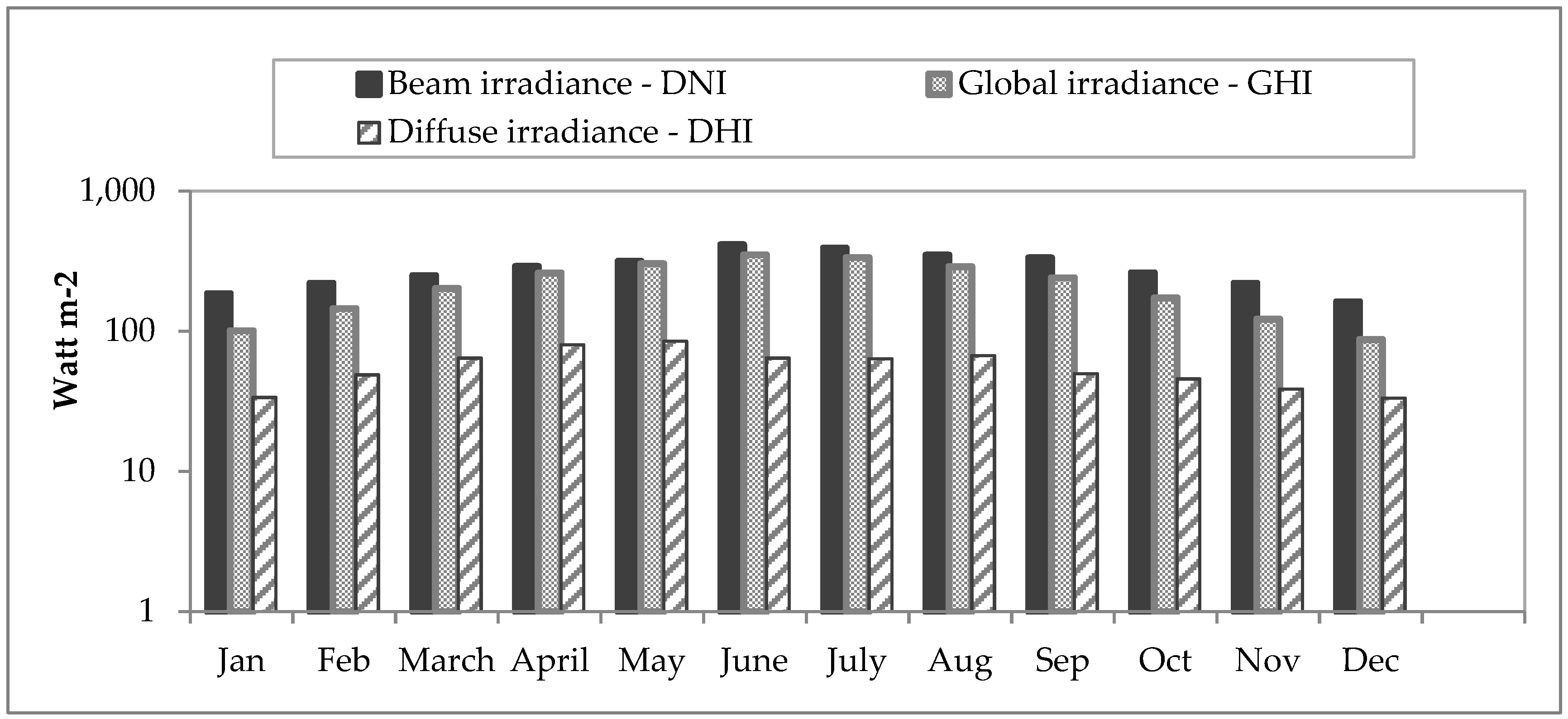
SAM was utilized for the modeling study of the PV system. For the techno-economic analysis, inputs to SAM included the site’s weather information; electric load data; and PV system design parameters related to the panel, inverter, and battery type, among others. The analysis period was 25 years. For the weather information input, the global, beam, and diffuse irradiance (typical meteorological year TMY3 data) for the selected location is shown in Figure 2. A self-shading analysis was performed manually using the criteria provided by [65], and a ground coverage ratio of 0.3 was shown to minimize self-shading. The electricity rate structure for the DWTP was downloaded from the utility rate database provided by SAM for Nevada. The rate structure applied was that of commercial facilities, with a demand range of 50–500 kW, or for an energy consumption greater than 10,000 kWh per month.

SAM was utilized to design the PV system. The desired array size and the inverter’s DC-to-AC ratio were provided as inputs for the design of the PV system. The module and inverter types were selected from the SAM database; their parameters were used to design the number of modules and inverters, and the system capacity. As the treatment plant operates 24 hours per day, battery storage was provided to meet the energy requirements in the absence of sunlight. SAM is equipped to model the vanadium redox flow, lead–acid, and lithium ion batteries. The battery storage (battery cells in series, and strings in parallel) was designed by providing the inputs of the desired bank capacity and the desired bank voltage. For the grid-connected PVs or PV systems coupled with energy storage, there were hundreds of possible design solutions, which depend on the selection of various technical and economic parameters. In this study, the optimal PV designs were chosen by running iterations using SAM, based on the possibilities of maximum PV energy generation outputs and lowest cost indicators.

Various states in the United States have adopted renewable portfolio standards (RPS), which require a certain portion of the state’s electricity to be generated using renewables. The Nevada RPS mandates that 25% of the total electricity the utility sells must be generated using renewables by the year 2025, of which 6% of the electricity must be generated using solar energy between 2016–2025. Because of the Nevada solar carve-outs, implementing distributed solar for residential, commercial, and industrial projects may qualify these for various financial incentives. For this study, financial incentives [59] were incorporated into the analysis. The Nevada state incentive of property tax exemption was applied for this analysis. Because of the conditions stipulated in the property tax exemption incentive, other state incentives such as the partial sales tax reduction of 2.6% could not be claimed. A federal investment tax credit (ITC) of 30% was also included in the analysis, however solar projects placed after 2022 can only claim an ITC of 10%.

For the economic assessment, the main indicators used were the net present value (NPV) and the levelized cost of energy (LCOE). NPV provides the present value of the net cash flows of a project over its design life. A positive NPV is indicative of a profitable project, whereas a negative NPV indicates a non-viable project. The estimation of the NPV includes the input parameters of the taxes and incentives, which may complicate the estimation of more simplistic metrics, such as the payback period. LCOE is the present value of the cost of the energy generated by the PV system over its design life, and is useful for making financial decisions when comparing PVs with other renewables or with an electric utility. The LCOE value is affected by the capital costs, incentives, depreciation method selected, operation and maintenance (O&M) costs, insurance costs, property taxes, and debt costs, as well as the salvage value of the project. The LCOE can be real or nominal, based on whether it was adjusted for inflation. Because the real LCOE is adjusted for inflation, it is typically used for long-term analyses, while the nominal LOCE is used for short-term analyses. The NPV and LCOE can be estimated using the following equations:

$$\mathrm{NPV}={\displaystyle \sum }_{\mathrm{t}=1}^{\mathrm{T}}\frac{{\mathrm{I}}_{\mathrm{t}}}{{\left(1+\mathrm{r}\right)}^{\mathrm{t}}}-{\mathrm{C}}_{\mathrm{O}}$$

(1)

where Co is the investment costs, I_t is the net cash inflows for time period t, T is the project’s life term, and r is the discount rate; and

$$LCOE =\frac{{{\displaystyle \sum }}_{t=0}^T\frac{C_t}{{\left(1+r\right)}^t}}{{{\displaystyle \sum }}_{t=1}^T\frac{Q_t}{{\left(1+r\right)}^t}}$$

(2)

where C_t is the cost for time period t, and Q_t is the energy generation in kWh in time period t.

4.3. Land Requirements

The available landholdings for the DWTP were determined using ArcMap software. The landholdings were compared against the land area requirements of the solar PV estimated by SAM.

4.4. Carbon Emissions

The direct carbon emissions for solar PVs are negligible during the operation of the system. However, there are emissions during the manufacturing and transportation of the panels, and during the construction or disintegration of a solar facility [66]. The net reduction in carbon emissions was estimated for this study by deducting the emissions generated before incorporating the PV, from the emissions generated after incorporating the PV, in order to offset the energy consumption of the DWTP. The product of the electricity source distribution (Table 2) and the median emission estimates data in gCO₂eq kWh⁻¹, provided by [45], was used to estimate the carbon emissions for the DWTP for the non-PV based design.

5. Results and Discussion

One of the objectives of this study was to use energy-driving units as the basis to establish energy consumption in the DWTP. The determined energy consumption was then used as an input for the SAM modeling study to simulate the performance of the solar PV, with and without battery storage, for meeting the electricity requirements of the plant. The results of this study include the actual design of the unit processes of the DWTP, the determination of the associated energy consumption (Section 5.1), and simulating the techno-economic performance of a PV system as an energy source for the DWTP (Section 5.2).

5.1. Unit Process Design and Energy Consumption of the DWTP

The water demand for the city is met by withdrawing water from seven groundwater wells, which are delivered and combined at the DWTP. At first, the groundwater undergoes coagulation. The addition of chemicals to the water requires metering pumps (

Table 5. Energy consumption estimations for the selected drinking water treatment plant.

s.no.	Unit Process	Sub-Processes	Energy Driving Unit	Plant Motor Size (hp)	Estimated Motor Size (hp)	Energy Consumption (kWh day−1)	Energy Intensity (Wh m−3)	Efficiency (%)
1.	Coagulation	Coagulant addition	Metering pump	0.5	0.5	1.8	0.05	0.76
		Polymer addition	Metering pump	0.5	0.5	1.8	0.05	0.76
		Acid addition	Metering pump	0.5	0.5	1.8	0.05	0.76
2.	Filtration		Surface wash pumps	-	4.5	5.5	0.15	0.74
			Backwash water transfer pumps	7.5	7.5	20.9	0.57	0.76
3.	Chlorination	Chlorine addition	Metering pumps	0.5	0.5	1.8	0.05	0.76
4.	Lime addition		Lime mixer	0.5	0.5	11.3	0.31	0.8
			Lime feed pump	1.5	1.3	22.8	0.62	0.76
5.	Lamella clarifier		Polymer pump	0.5	0.5	1.8	0.05	0.76
			Sludge transfer pumps	-	3.5	2.7	0.07	0.72
6.	Water reclamation basins		Water transfer pumps	25	25	18.7	0.51	0.76
7.	Filter press		Filter aid pumps	0.25	0.2	0.94	0.03	0.76
			Filter press and feed pump	6	5	21	0.57	-
8.	Booster pumps		Pump #1	200	187	3.33 × 103	90.7	0.8
			Pump #2	125	123	2.20 × 103	59.9	0.8

). Two metering pumps were provided for each chemical addition, where one was reserved as a backup. The flow rate for the chemicals was taken as 0.023 m³ hour⁻¹, 0.18 m³ hour⁻¹, and 0.001 m³ hour⁻¹ for the addition of coagulant, sulfuric acid, and polymer, respectively—these flow rates were provided by the DWTP managers (Table 5).

The water filtration required 16 multi-media filters including an extra filter to incorporate redundancy. A filtration rate of 10 m hour⁻¹ was used. The filters were backwashed once per day for 15 min. The energy-consuming units in the filtration were surface wash pumps, applied for a duration of 5 min, and backwash water transfer pumps (Table 5). The filter-to-waste time was 15 min, and the filtration recovery was 96%. After the filters were backwashed, the backwash water was stored in a 134 m³ basin before being pumped to lamella clarifiers for dewatering. After the water was filtered, it was chlorinated. A 1020 m³ contact basin with eight pass-around-the-end baffles provided 1 h of detention time based on the average flow conditions, as recommended by the USEPA, for the adequate mixing of sodium hypochlorite with the treated water. A residual chlorine concentration of 1.6 mg L⁻¹ was provided to ensure protection against possible microbial contamination within the water distribution system.

Lime was added to lower the water pH to 7.8. For the mixing of the lime slurry, a velocity gradient of 900 s⁻¹ and a detention time of 30 s were used. Two booster pumps were provided to transport water to elevated storage tanks, and two additional pumps were provided as a backup. The energy consumption for the booster pumps was found to be 5.53 MWh day⁻¹ (Table 5).

The backwash water was treated using a lamella clarifier and belt-filter presses. Two lamella clarifiers were provided. Each clarifier was designed for a surface loading rate of 5 m h⁻¹, and was sized to have a volume of 50 m³. The sludge was transferred, using pumps, to two sludge storage basins to be further treated by the filter presses. Two filter presses were provided. The sludge underwent solid/liquid separation using one of the filter presses, and the other press was used as a backup. The filter press (of capacity 0.3 m³) was sized for a belt width of 1 m. Based on the characteristics of the sludge cake and the waste filtrate produced in the dewatering operation, both were classified as non-hazardous. The sludge cake was transported to a landfill for disposal, while the filtrate was disposed of in the sewer.

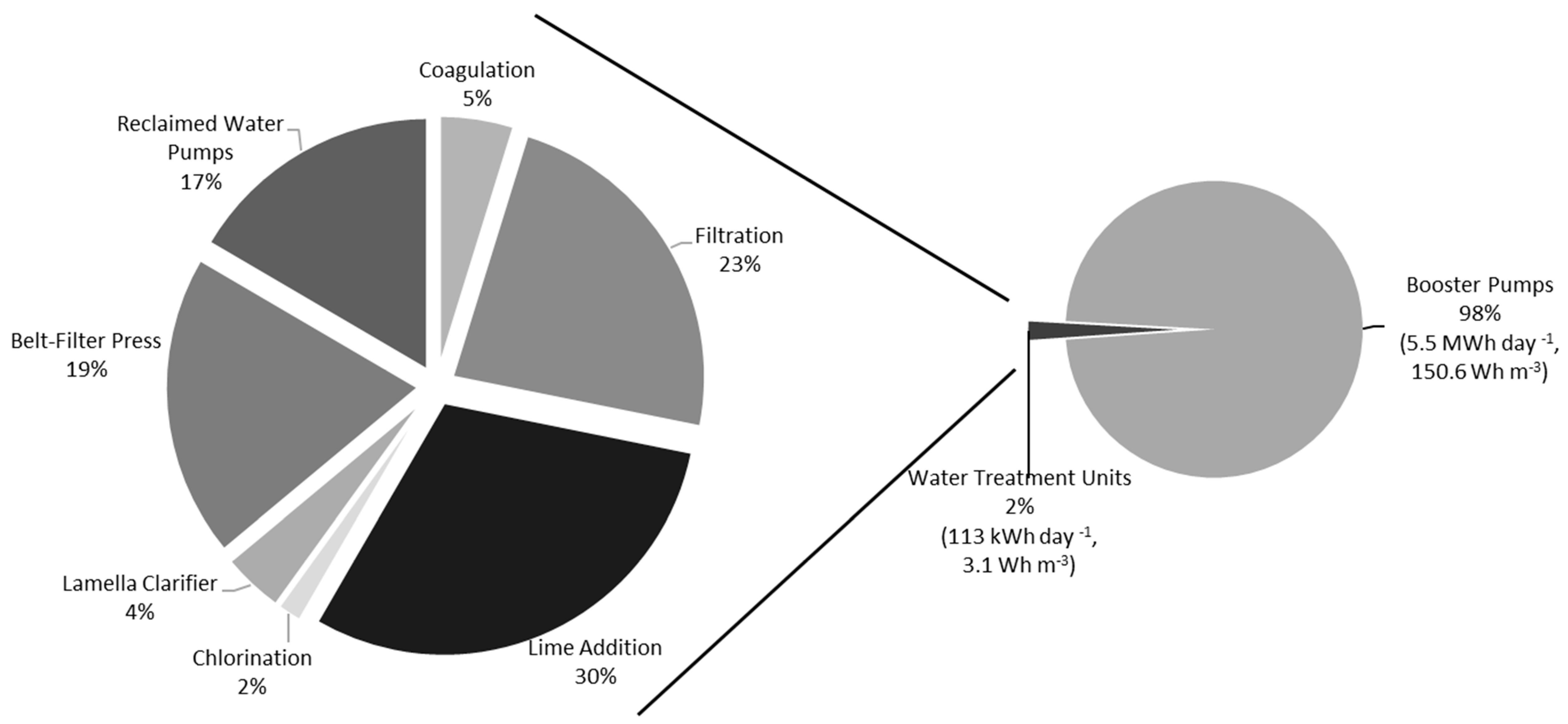
The total operational energy consumption of the DWTP was 5.6 MWh day⁻¹, which consisted of the energy consumption for the water treatment units (113 kWh day⁻¹) and the booster pumps (5.5 MWh day⁻¹). The motor sizes determined for the DWTP were validated against the actual motor sizes of the plant provided by the DWTP managers, and were found to be in good agreement with the estimated sizes (Table 5). Overall, the booster pumps and the unit processes of the DWTP utilized about 98% and 2% of the overall energy consumption of the DWTP, respectively (Figure 3). Hence, the largest consumer of energy is the pumping operation for the DWTP (Figure 3 and Table 5), corresponding to 80.5 kWh day⁻¹ for the pumping operation within the plant, and 5.5 MWh day⁻¹ for the booster pumps for water storage.

The second largest consumer of energy was the process of lime addition, which consisted of lime mixing and lime feed pumps, followed by the filtration process. The largest energy intensity was 0.58 Wh m⁻³ for the backwash water transfer pumps and the filter press, and 0.63 Wh m⁻³ for the lime feed pumps (Table 5). Overall, for the water treatment units, the energy intensity was determined to be 3.1 Wh m⁻³. The processes involving residual management, which included the operation of lamella clarifiers, the filter press, and reclaimed water pumps, were found to utilize 40% of the overall energy consumption of the DWTP. A sensitivity analysis was performed for the energy consumption estimates related to the pumping operation for the treatment plant. The wire-to-electric efficiencies of the pumps were increased by 5% and 10%, which resulted in a 4.8% (107.5 kWh day⁻¹) and 9.1% (102.6 kWh day⁻¹) decrease in the total operational energy consumption (113 kWh day⁻¹) of the water treatment units, respectively. However, decreasing the wire-to-water efficiencies by 5% (118.8 kWh day⁻¹) and 10% (125.4 kWh day⁻¹) resulted in increased total operational energy consumption by 5.3% and 11.1%, respectively.

Various studies have reported energy consumption estimates for drinking water treatment. Ref. [7] reported on electricity use for a typical urban water system in Northern California for water supply and transport (0.04 kWh m⁻³), water treatment (0.026 kWh m⁻³), and water distribution (0.32 kWh m⁻³), amounting to approximately 0.38 kWh m⁻³ of the total electricity use. Ref. [67] conducted a literature review of various water-related life cycle processes, and their associated energy requirements. The study reported the energy consumption of various energy driving units of water treatment processes and operations. This included rapid mixers for coagulation (0.008–0.022 kWh m⁻³), dissolved air flotation systems (9.5–35.5 W h m⁻³), gravity filtration (0.005–0.014 kWh m⁻³), and ozone generation (0.2 kWh m⁻³).

5.2. System Advisor Model

The results for the techno-economic analysis using SAM are shown in

Table 6. Technical and economic analysis results for the solar PV system with and without battery storage by using SAM for the drinking water treatment plant. A sensitivity analysis for the standalone PV system shown by using different types of tracking mechanisms for the PV system (the values of the affected parameters are shaded in grey).

PV System Components	Parameter	Unit	Standalone PV System with Battery Storage (100% of Electric Load Offset)			Grid-connected PV with No Battery Storage (60% of Electric Load Offset) (Two-Axis Tracking)
			2-Axis Tracking	1-Axis Tracking	Fixed
Module	Nameplate capacity	kWdc	1500	1535	1810	1500
	Number of modules	-	5769	5904	6957	5769
	Modules per string	-	9	9	9	9
	Strings in parallel	-	641	656	773	641
	Total module area	×103 m²	9.4	9.7	11.4	9.4
	String (Voc)	Volt	340	340	340	340
	String (Vmp)	Volt	280	280	280	280
	Total land area	×103 m²	31.6	32.4	38.0	31.6
Inverter	Total capacity	kWdc	1309.7	1343.3	1582.6	1309.7
	Number of inverters	-	312	320	377	312
	Maximum DC voltage	Voltdc	480	480	480	480
	Minimum MPPT voltage	Voltdc	100	100	100	100
	Maximum MPPT voltage	Voltdc	480	480	480	480
	DC to AC Ratio	-	1.2	1.2	1.2	1.2
Battery	Nominal bank capacity	MWh	30	30	30	-
	Nominal bank voltage	×103 Volt	350	350	350	-
	Cell in series	-	175	175	175	-
	Strings in parallel	-	72	72	72	-
	Battery efficiency	%	89.6	89.6	89.6	-
Financial Metrics	Net present value Levelized cost of electricity (nominal)	$ million Cents kWh−1	0.56 3.05	0.56 3.19	0.45 3.98	1.05 0.48
	Levelized cost of electricity (real)	Cents kWh−1	2.47	2.58	3.22	0.39
	Net capital cost	$ million	9.16	9.17	9.78	3.93
	Electricity bill without system (year one)	$ million	0.206	0.206	0.206	0.206
	Electricity bill with system (year one)	$	192	192	192	46,684

. The energy consumption associated with the unit processes of the DWTP and booster pumps for water distribution, was the electric load input for the SAM. The results of the modeling study are as follows.

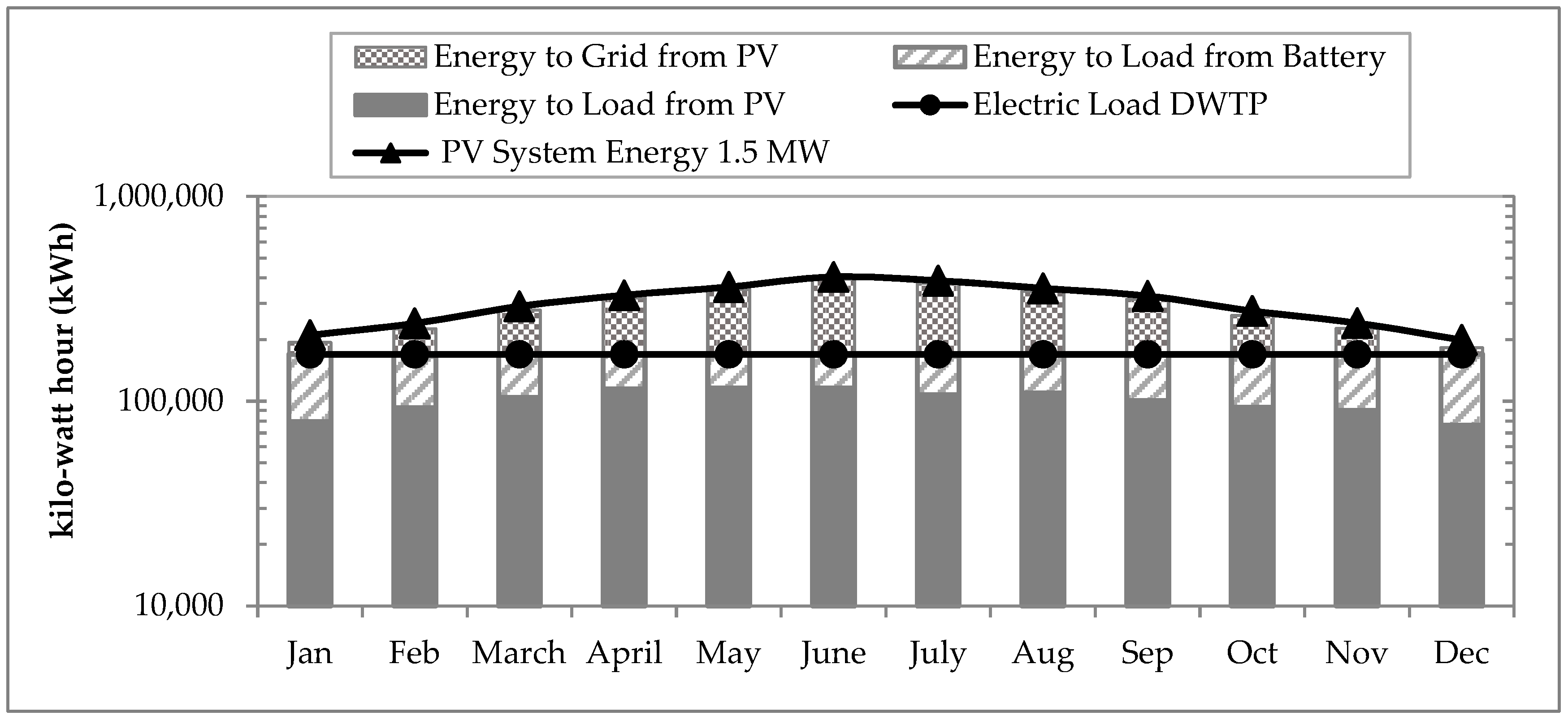
Hundreds of PV system designs are possible, with and without battery storage. However, the optimal PV system designs, dependent on the input of the selected technical and economic parameters, were chosen by running iterations using SAM. The desired PV array size was changed in increments of 5 kW while using a DC-to-AC ratio of 1.2, and the desired battery bank capacity was changed in increments of 50 kWh while using a bank voltage of 350 V. The optimal designs selected in SAM were representative of the lowest possible cost solutions. The PV system (1.5 MW) with battery storage (30 MWh) was designed as a stand-alone system to meet 100% of the load for the 24 h duration of the day. The NPV was found to be positive (Table 6). Moreover, a similar PV system with no battery storage, but that was grid-connected, would offset about 60% of the total load, with a NPV of $1 million (Table 6), thus showing the effect of the battery storage on the performance and cost of the system. Figure 4 shows the electric load input and the energy generation output of the PV system for the DWTP.

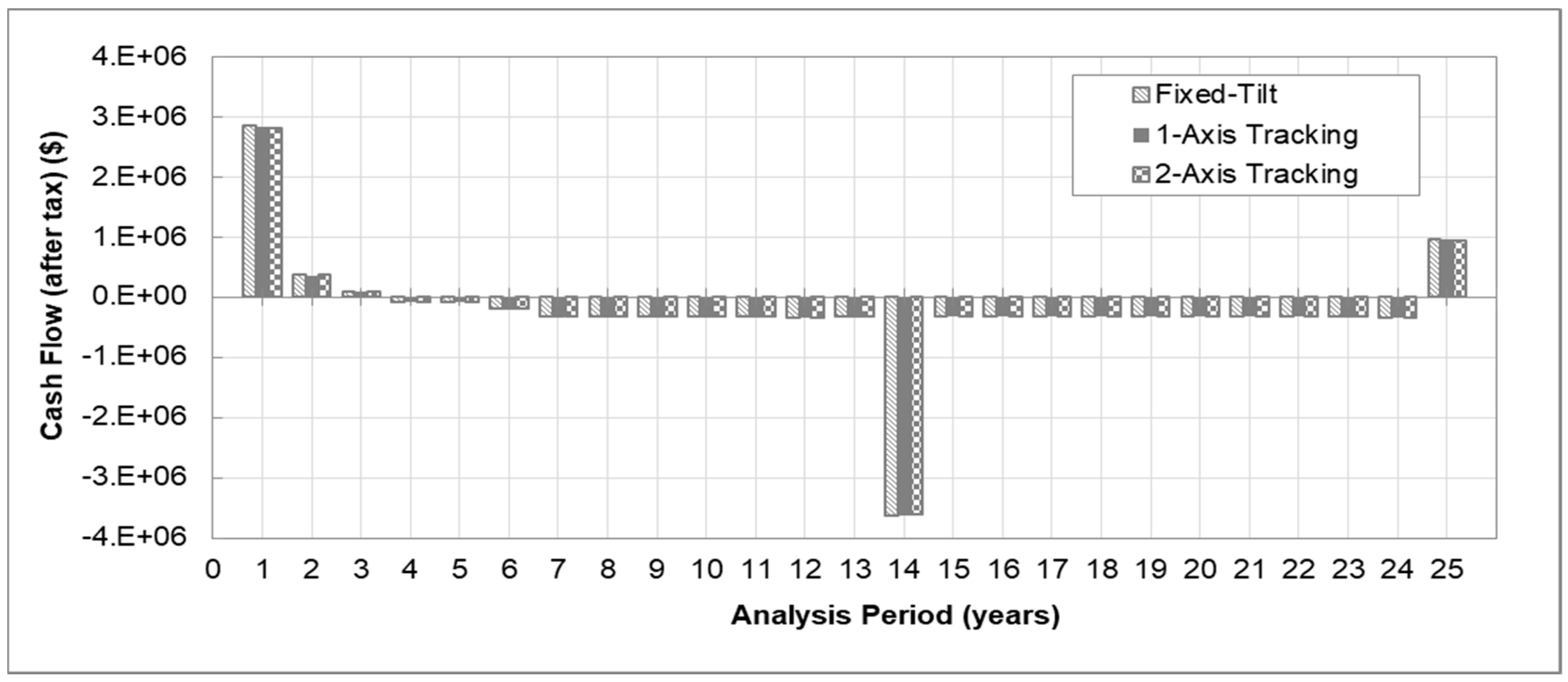
A sensitivity analysis was conducted by changing the tracking type of the PV system (Table 6). Changing the tracking mechanism from two-axis to one-axis did not greatly affect the performance and economics of the PV system, however the fixed PV system was shown to be a relatively costly choice. Based on the economic indicators, the standalone PV system with two-axis tracking was found to be the most cost-effective (Table 6). The cash flow diagram for the fixed tilt, one-axis, and two-axis tracking is shown in Figure 5. Table 6 shows a $192 fixed yearly charge for maintaining grid-connection, to be used as a backup for the stand-alone PV system, as providing other types of backup systems for electricity generation would be much more expensive.

In the current study, a 1.5 MW solar PV coupled with 30 MWh of battery storage was able to offset 100% of the energy consumption of the DWTP. Ref. [39] utilized PVs and wind turbines coupled with battery storage to offset the energy consumption of a DWTP treating 3.11 m³ of water per second, located in Netherlands. This study modeled several stand-alone scenarios, including a 5.6 MW PV system, and 8 MW wind turbines coupled with 60 MWh battery storage to meet 96% of the energy demand; however, 100% of the energy demand could not be met, because the massive size of the battery deemed it uneconomical. Furthermore, without battery storage, the system was able to meet 88% of the energy demand.

The manual dispatch model selected in SAM aims to minimize purchases from the grid. It first tries to meet the load with PV, next the battery, and then the grid. For the selected option, only the solar PV charged the battery after meeting the load. Furthermore, for this analysis, the battery bank was replaced after 13 years, and for the replacement, the battery cost was reduced by 30%. This is because various studies predicted a decrease in battery storage costs [68,69]. Ref. [69] forecasted battery storage costs to fall by 39% between the years 2016–2020. Hence, a value of 30% was used as a conservative estimate for this study. While battery storage prices are continuing to fall, current battery prices remain relatively high. Presently, the high cost of battery storage poses a major constraint for using solar as a source for a 24 h supply of energy.

Regarding the inclusion of time resolved demands, for most components of energy demand, the periods of high and low demand have to be taken in consideration when modeling the integration of renewables, which are typically intermittent energy sources. Ref. [70] took into account the time demand variability when computing the energy demand for household appliances, while [71] used hydroelectric power to buffer intermittent renewable energy in California, and included the time variation of the demand. However, DWTPs typically do not operate 24 h a day, because most communities must have treated water storage capacity for at least three days. In addition, many DWTPs in the United States currently operate at night for 8 to 10 h to avoid peak demand times, to reduce the cost of treatment. Furthermore, DWTPs are built with flexibility and the design of unit processes incorporates a significant down time for maintenance operations. Contrary to the energy demand and dispatch for most components of a city (e.g., hospital and household), the energy demand for DWTP does not experience the same time demand issues, because they can operate at night or during periods of low demand, as they have storage capacity and redundancy of unit operations. However, throughout the world, water treatment is not performed in the same way, and the energy mix and time of operation may require an evaluation of the demand at different times of the day, which thus requires the integration of this demand to the evaluation. The time resolved energy demand was not evaluated in this study for the reasons mentioned above.

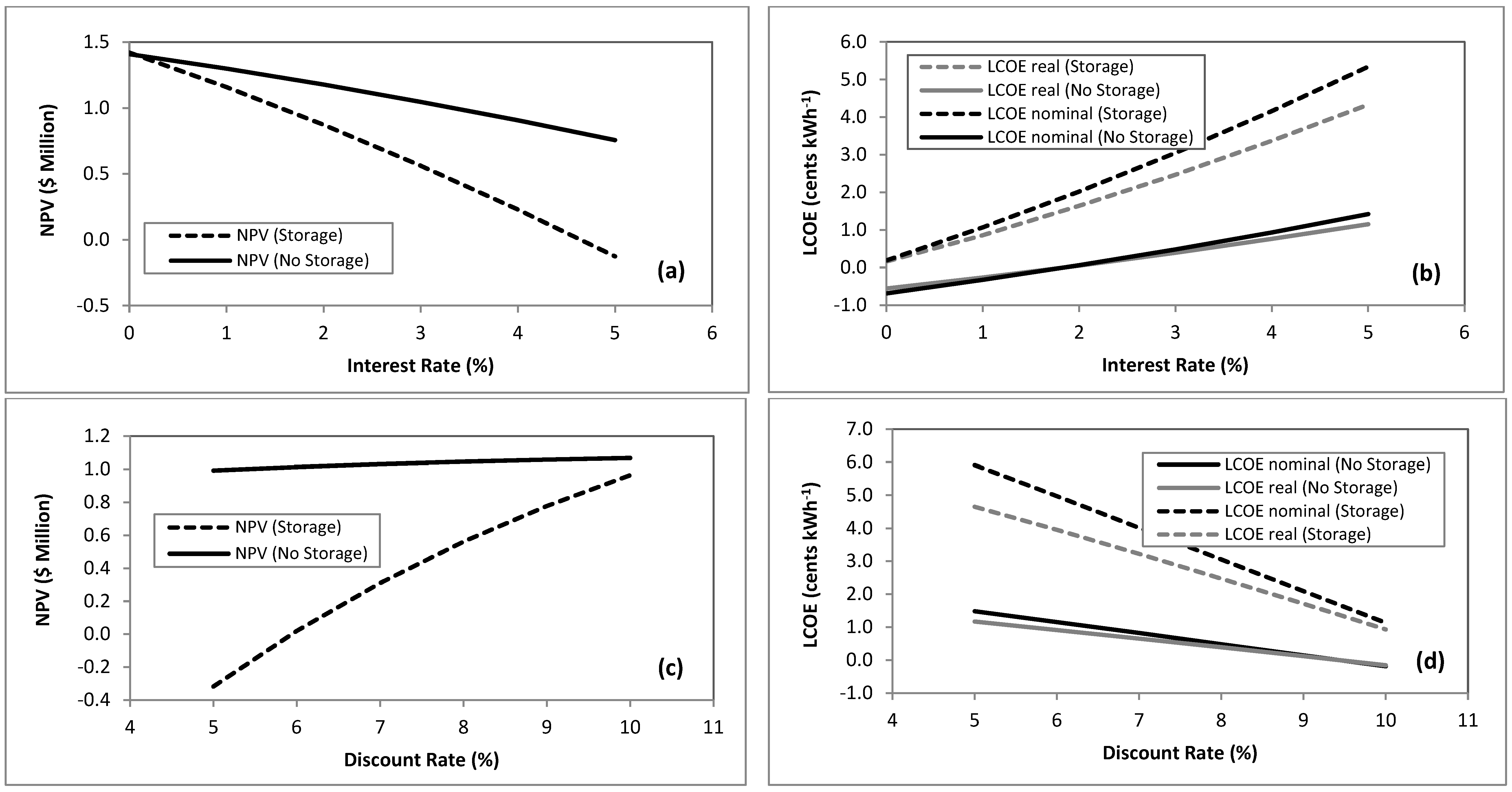
The LCOE for the current study ranged between 3–4 cents kWh⁻¹. The LCOE equations provided by [22,72] were also used to generate LCOE values, which were found to be very close to the LCOE generated using SAM; for example, for a one-axis PV, the nominal LCOE was found to be 3.16 cents kWh⁻¹ against the SAM-calculated LCOE of 3.19 cents kWh⁻¹, whereas the real LCOE was found to be 2.56 cents kWh⁻¹ against the SAM-calculated LCOE of 2.58 cents kWh⁻¹. Ref. [73] reported a LCOE value of 4.9 cents kWh⁻¹ for a 30.5 MW PV plant at Springerville, AZ, and this value was estimated in 2006. Ref. [74] reported a LCOE value of 5.9 and 2.8 cents kWh⁻¹ when the ITC was included, and 8 and 4.1 cents kWh⁻¹ when the ITC was not included for commercial- and utility-scale PV installation, respectively, in Phoenix, Arizona. Investors heavily use the values of LCOE and NPV to make financial decisions; however, these indicators have certain shortcomings. The parameters of NPV do not take into account the scale of investment, and rely on the value of the discount factor. The LCOE estimate is dependent on the selection of various financial parameters, and hence any error in assuming those financial parameters will affect the true LCOE estimate. A sensitivity analysis was conducted by quantifying the effect of the discount rate and interest rate on the LCOE and NPV for the DWTP (Figure 6).

Technological improvements have increased the energy output of solar panels and decreased their costs. However, the successful deployment of solar still depends largely on federal and state incentives, as in the case of this study. The effect of the financial incentives on the NPV and LCOE was evaluated by not incorporating (a) the 30% ITC (NPV negative; LCOE 10.73 cents kWh⁻¹), (b) property tax exemption incentive (NPV positive; LCOE 4.88 cents kWh⁻¹), and a (c) combination of (a) and (b) (NPV negative; LCOE 12.08 cents kWh⁻¹). However, if these financial incentives were retained for the analysis (Table 6), a comparison of the results indicated the favorable influence of financial incentives for solar implementation. Thus, governmental policies and incentives may help remove financial barriers, boost investment, and facilitate solar power development. The provision of financial incentives could be a motivating factor for the water sector in order to incorporate renewables into the design of the water infrastructure. Priority dispatch for renewables, feed-in-tariffs, and net metering also encourage the installation of renewables [75,76].

The successful solar energy projects pursued in recent years are grid-connected PVs, as well as those coupled with energy storage, and are the driving force behind the success of solar energy. Ref. [77] conducted a techno-economic assessment for a PV-based water treatment (using reverse osmosis) and pumping system in semi-arid Fortaleza, Brazil. The study found that the optimum system configuration would involve a cutoff concentration of 2748 mg L⁻¹ of brackish water when using PV panels with no battery storage, which resulted in a drinking water production of 175 L/day⁻¹ at a 324.60 mg L⁻¹ salt concentration. Ref. [78] conducted an economic assessment study of three power sources (grid, diesel, and PV) for the well pumping and desalination of brackish groundwater in Jordan. The study found the PV-powered system to be more cost-effective when compared with a diesel-powered system, but less cost-effective compared with a grid-connected system. Ref. [79] analyzed the technical feasibility of brackish water treatment for a small village in Jordan with no access to electricity. A hybrid energy system was proposed, comprised of 2 kW of solar PV, a 10 kW wind system, and a 13 kW hydro-system, resulting in the production of 40 m³ day⁻¹ of drinking water.

5.3. Land Requirements

For PV implementation, the land area requirements were found to be 0.03 and 0.04 km² for the two-axis and fixed PVs, which is equivalent to six and eight football fields, respectively (Table 6). The existing landholdings of the treatment plant were estimated, using ArcMap, as 0.17 km². Hence, the land acquirement was not required for the development of the distributed solar. The land utilized for the analysis was relatively flat, with low shrubs and grass; thus, the existing condition of the land area did not warrant significant work related to land preparation for solar development.

5.4. Carbon Emissions

The net reduction in carbon emissions was found to be 0.950 and 0.570 million kg CO₂eq year⁻¹ (0.07 and 0.04 million kg CO₂eq m⁻³) for the DWTP with and without battery storage (for two-axis tracking PV), respectively. Ref. [80] detailed the average carbon emissions for 36 Chilean DWTPs as 0.11 million kg CO₂eq year⁻¹. Ref. [81] analyzed four DWTPs in the city of Toronto, and reported an average value of 15.3 million kg CO₂eq year⁻¹ for the four plants. Even though the initial investment costs are large for PVs, the reduction in emissions due to their development leads to a healthier community and environment. Ref. [82] estimated a reduction in carbon emissions as 0.4 million kg CO₂eq year⁻¹ for using PVs and wind energy for a DWTP located in Phoenix, Arizona. Incorporating distributed solar in a water infrastructure can lead to the decarbonization of water operations.

The current study satisfactorily achieved the desired objectives. However, this work has certain limitations related to the energy efficiency analysis. Energy efficiency measures’ implementation in plants, such as installing variable speed pumps and more efficient motors, have not been explored in this research. This is because of the unavailability of data for validation. Most DWTPs in the United States, despite being very modern in terms of their unit operations, do not have individual energy meters for specific units. Rather, they have energy totalizers for some parts of the plant, or sometimes only a total energy meter for the entire plant. Notwithstanding the availability of actual data for validation, a sensitivity analysis was performed for the efficiency of the pumping operation for the treatment plant, as discussed in Section 5.1. Furthermore, for the PV system, a sensitivity analysis related to the efficiency values could not be performed. This is because the module and inverter types were selected from the database provided by the SAM. Once a selection was made, the efficiencies related to the PV system could not be modified. However, we did include a sensitivity analysis for the PV system by changing the types of tracking mechanisms of the PVs (two-axis, one-axis, and fixed PVs).

One of the strengths of the current work was the analysis of the drinking water treatment process, which specified the energy requirement of each sub-process, as well as using the SAM model to simulate the required solar PV capacity and storage requirements to meet the energy demand. Limited literature exists for analyzing the energy consumption of drinking water treatment plants. Fundamental design equations focusing on each energy-consuming unit were used to arrive to a motor size that is run in order to power the unit. By calculating the energy use of the unit processes, this method can be used for other plants at different locations. The design equations used for this study can be applied to determine the energy consumption of other plants, while the energy intensity estimates could be used to compare the performance of a plant against other DWTPs. We believe that this work presents valuable insights to researchers in the field and to policy makers.

6. Conclusions

The energy consumption and energy intensity values were determined by designing an existing small DWTP (validated using the plant’s data). The processes designed were coagulation (0.15 Wh m⁻³), filtration (0.72 Wh m⁻³), chlorination (0.05 Wh m⁻³), lime mixing (0.93 Wh m⁻³), booster pumps (150.6 Wh m⁻³), and residual management processes, which included water reclamation basins (0.51 Wh m⁻³), a lamella clarifier (0.12 Wh m⁻³), and a filter press (0.6 Wh m⁻³). The pumping operation was determined as the largest consumer of energy for the DWTP, as the operational energy consumption was found to be the largest for the booster pumps for water storage (150.6 Wh m⁻³). The treatment of the drinking water (excluding booster pumps) utilized 2% of the total operational energy consumption (3.1 Wh m⁻³). Overall, the processes of lime addition and filtration were the largest consumers of energy for the water treatment units (0.93 and 0.72 Wh m⁻³, respectively). The design equations used for this study can be applied to determine the energy consumption of other plants, while the energy intensity estimates could be used to compare the performance of the plant against other DWTPs.

The techno-economic performance of the proposed PV system was conducted using SAM to offset the energy consumption of the DWTP; the modeling study determined that the DWTP would require a 1.5 MW solar PV with a battery bank capacity of 30 MWh to act as a standalone system. The NPV for the PV system in standalone mode was found to be positive, and the LCOE was found between 3–4 cents kWh⁻¹. A similar PV system without battery storage, but that was grid-connected, would offset about 60% of the total load. The techno-economic performance of the tracking PV was better when compared to the fixed tilt PV system. The existing landholdings of the plant (0.17 km²) were found to be sufficient to meet the land area requirements (0.03 km²) for the installation of the PV system. The net reduction in carbon emissions was 950 and 570 metric tons of CO₂eq year⁻¹ due to the PV-based design, with and without battery storage, respectively. The methodology used in this research can be applied to other treatment plants, with appropriate modifications, for using PVs to offset energy requirements of the plant, to help achieve sustainability goals, energy independence, and reduced carbon emissions.

References

- Shrestha, E.; Ahmad, S.; Johnson, W.; Shrestha, P.; Batista, J.R. Carbon footprint of water conveyance versus desalination as alternatives to expand water supply. Desalination 2011, 280, 33–43. [Google Scholar] [CrossRef]
- Shrestha, E.; Ahmad, S.; Johnson, W.; Batista, J.R. The carbon footprint of water management policy options. Energy Policy 2012, 42, 201–212. [Google Scholar] [CrossRef]
- Foley, A.; Olabi, A.G. Renewable energy technology developments, trends and policy implications that can underpin the drive for global climate change. Renew. Sustain. Energy Rev. 2017, 68, 1112–1114. [Google Scholar] [CrossRef] [Green Version]
- Karas, D.E.; Byun, J.; Moon, J.; Jose, C. Copper-oxide spinel absorber coatings for high-temperature concentrated solar power systems. Sol. Energy Mater. Sol. Cells 2018, 182, 321–330. [Google Scholar] [CrossRef] [Green Version]
- Lin, B.; Ahmad, I. Analysis of energy related carbon dioxide emission and reduction potential in Pakistan. J. Clean. Prod. 2017, 143, 278–287. [Google Scholar] [CrossRef]
- Spellman, F.R. Water & Wastewater Infrastructure: Energy Efficiency and Sustainability; CRC Press: Boca Raton, FL, USA, 2013. [Google Scholar]
- Klein, G.; Krebs, M.; Hall, V.; O’Brien, T.; Blevins, B. California’s Water–Energy Relationship; California Energy Commission: Sacramento, CA, USA, 2005. [Google Scholar]
- Bailey, J.R. Investigating the Impacts of Conventional and Advanced Treatment Technologies on Energy Consumption at Satellite Water Reuse Plants. UNLV Theses 1707, University of Nevada Las Vegas, Las Vegas, NV, USA, 2012. [Google Scholar]
- Newell, T.S. The Impact of Advanced Wastewater Treatment Technologies and Wastewater Strength on the Energy Consumption of Large Wastewater Treatment Plants. UNLV Theses 1764, University of Nevada Las Vegas, Las Vegas, NV, USA, 2012. [Google Scholar]
- Molinos-Senante, M.; Sala-Garrido, R. Energy intensity of treating drinking water: understanding the influence of factors. Appl. Energy 2017, 202, 275–281. [Google Scholar] [CrossRef]
- Molinos-Senante, M.; Sala-Garrido, R. Evaluation of energy performance of drinking water treatment plants: Use of energy intensity and energy efficiency metrics. Appl. Energy 2018, 229, 1095–1102. [Google Scholar] [CrossRef]
- Wen, H.; Zhong, L.; Fu, X.; Spooner, S. Water Energy Nexus in the Urban Water Source Selection a Case Study from Qingdao; Water Resources institute: Beijing, China, 2014. [Google Scholar]
- Dawadi, S.; Ahmad, S. Evaluating the impact of demand-side management on water resources under changing climatic conditions and increasing population. J. Environ. Manag. 2013, 114, 261–275. [Google Scholar] [CrossRef]
- US Census Bureau. 2012. Available online: http://www.census.gov/popest/data/historical/index.html (accessed on 15 October 2016).
- USEPA. U.S. Environmental Protection Agency. 2016. Available online: https://www3.epa.gov/region9/waterinfrastructure/ (accessed on 15 October 2016).
- Goldstein, R.; Smith, W. Water & Sustainability: US Electricity Consumption for Water Supply & Treatment-the Next Half Century; Electric Power Research Institute: Palo Alto, CA, USA, 2002; Volume 4. [Google Scholar]
- Sanders, K.T.; Webber, M.E. Evaluating the energy consumed for water use in the United States. Environ. Res. Lett. 2012, 7, 034034. [Google Scholar] [CrossRef]
- Pirnie, M. Statewide Assessment of Energy Use by the Municipal Water and Wastewater Sector; Report 08-17; New York State Energy Research and Development Authority NYSERDA: Albany NY USA, 2008. [Google Scholar]
- Strazzabosco, A.; Kenway, S.J.; Lant, P.A. Solar PV adoption in wastewater treatment plants: A review of practice in California. J. Environ. Manag. 2019, 248, 109337. [Google Scholar] [CrossRef]
- Yaqoot, M.; Diwan, P.; Kandpal, T.C. Review of barriers to the dissemination of decentralized renewable energy systems. Renew. Sustain. Energy Rev. 2016, 58, 477–490. [Google Scholar] [CrossRef]
- Wadhawan, S.R.; Pearce, J.M. Power and energy potential of mass-scale photovoltaic noise barrier deployment: A case study for the US. Renew. Sustain. Energy Rev. 2017, 80, 125–132. [Google Scholar] [CrossRef] [Green Version]
- Kang, M.H.; Rohatgi, A. Quantitative analysis of the levelized cost of electricity of commercial scale photovoltaics systems in the US. Sol. Energy Mater. Sol. Cells 2016, 154, 71–77. [Google Scholar] [CrossRef]
- Lai, C.S.; McCulloch, M.D. Levelized cost of electricity for solar photovoltaic and electrical energy storage. Appl. Energy 2017, 190, 191–203. [Google Scholar] [CrossRef]
- Denholm, P.; Drury, E.; Margolis, R. Solar Deployment System (Solar DS) Model: Documentation and Sample Results (No. NREL/TP-6A2-45832); National Renewable Energy Lab. (NREL): Golden, CO, USA, 2009. [Google Scholar]
- Fosnight, E.A.; Wood, E.; El Gayar, O.; Stackhouse, P.; Michels, L. The Solar and Wind Energy Resource Assessment (SWERA) Decision Support System (DSS) Benchmarking Report. 2010. Available online: https://www.nasa.gov/sites/default/files/files/CL-SWERA_benchmarking_report_29sep2010_finalWEB.pdf (accessed on 7 October 2016).
- Dobos, A.; Neises, T.; Wagner, M. Advances in CSP simulation technology in the System Advisor Model. Energy Procedia 2014, 49, 2482–2489. [Google Scholar] [CrossRef] [Green Version]
- Gilman, P.; Blair, N.; Mehos, M.; Christensen, C.; Janzou, S.; Cameron, C. Solar Advisor Model User Guide for Version 2.0; National Renewable Energy Lab. (NREL): Golden, CO, USA, 2008. [Google Scholar]
- Kang, M.H.; Kim, N.; Yun, C.; Kim, Y.H.; Rohatgi, A.; Han, S.T. Analysis of a commercial-scale photovoltaics system performance and economic feasibility. J. Renew. Sustain. Energy 2017, 9, 023505. [Google Scholar] [CrossRef]
- MacAlpine, S.; Deline, C.; Dobos, A. Measured and estimated performance of a fleet of shaded photovoltaic systems with string and module-level inverters. Prog. Photovolt. Res. Appl. 2017, 25, 714–726. [Google Scholar] [CrossRef] [Green Version]
- Tozzi, P., Jr.; Jo, J.H. A comparative analysis of renewable energy simulation tools: Performance simulation model vs. system optimization. Renew. Sustain. Energy Rev. 2017, 80, 390–398. [Google Scholar] [CrossRef]
- Bukhary, S. Water-Energy Nexus Approaches for Solar Development and Water Treatment in the Southwestern United States. Dissertation 3224, University of Nevada Las Vegas, Las Vegas, NV, USA, 2018. [Google Scholar]
- Mileva, A.; Johnston, J.; Nelson, J.H.; Kammen, D.M. Power system balancing for deep decarbonization of the electricity sector. Appl. Energy 2016, 162, 1001–1009. [Google Scholar] [CrossRef] [Green Version]
- Bukhary, S.; Ahmad, S.; Batista, J. Analyzing land and water requirements for solar deployment in the Southwestern United States. Renew. Sustain. Energy Rev. 2018, 82, 3288–3305. [Google Scholar] [CrossRef]
- Bukhary, S.; Chen, C.; Ahmad, S. Analysis of Water Availability and Use for Solar Power Production in Nevada. In World Environmental and Water Resources Congress; American Society of Civil Engineers: Reston, VA, USA, 2016; pp. 164–173. [Google Scholar]
- Bouhadjar, S.I.; Kopp, H.; Britsch, P.; Deowan, S.A.; Hoinkis, J.; Bundschuh, J. Solar powered nanofiltration for drinking water production from fluoride-containing groundwater—A pilot study towards developing a sustainable and low-cost treatment plant. J. Environ. Manag. 2019, 231, 1263–1269. [Google Scholar] [CrossRef] [PubMed]
- Chae, K.J.; Kang, J. Estimating the energy independence of a municipal wastewater treatment plant incorporating green energy resources. Energy Convers. Manag. 2013, 75, 664–672. [Google Scholar] [CrossRef]
- Garg, M.C.; Joshi, H. A review on PV-RO process: Solution to drinking water scarcity due to high salinity in non-electrified rural areas. Sep. Sci. Technol. 2015, 50, 1270–1283. [Google Scholar] [CrossRef]
- Nawarkar, C.J.; Salkar, V.D. Solar powered electrocoagulation system for municipal wastewater treatment. Fuel 2019, 237, 222–226. [Google Scholar] [CrossRef]
- Soshinskaya, M.; Crijns-Graus, W.H.; van der Meer, J.; Guerrero, J.M. Application of a microgrid with renewables for a water treatment plant. Appl. Energy 2014, 134, 20–34. [Google Scholar] [CrossRef] [Green Version]
- Bukhary, S.; Batista, J.; Ahmad, S. Evaluating the Feasibility of Photovoltaic-Based Plant for Potable Water Treatment. In World Environmental and Water Resources Congress; American Society of Civil Engineers: Reston, VA, USA, 2017; pp. 256–263. [Google Scholar]
- Bukhary, S.; Weidhaas, J.; Ansari, K.; Mahar, R.B.; Pomeroy, C.; Van Derslice, J.A.; Burian, S.; Ahmad, S. Using Distributed Solar for Treatment of Drinking Water in Developing Countries. In World Environmental and Water Resources Congress; American Society of Civil Engineers: Reston, VA, USA, 2017; pp. 264–276. [Google Scholar]
- Jaskolski, M.; Schmitz, L.; Otter, P.; Pellegrino, Z. Solar-powered drinking water purification in the oases of Egypt’s Western Desert. J. Photonics Energy 2019, 9, 043107. [Google Scholar] [CrossRef]
- USEPA. U.S. Environmental Protection Agency. 2016. Available online: https://www.epa.gov/sites/production/files/2016-08/documents/scienceinaction_small_systems_final-508.pdf (accessed on 20 October 2017).
- Crittenden, J.C.; Trussell, R.R.; Hand, D.W.; Howe, K.J.; Tchobanoglous, G. MWH’s Water Treatment: Principles and Design; John Wiley & Sons: Hoboken, NJ, USA, 2012. [Google Scholar]
- Moomaw, W.; Burgherr, P.; Heath, G.; Lenzen, M.; Nyboer, J.; Verbruggen, A. Annex II: Methodology. In IPCC Special Report on Renewable Energy Sources and Climate Change Mitigation; Edenhofer, O., Pichs-Madruga, R., Sokona, Y., Seyboth, K., Matschoss, P., Kadner, S., Eds.; Cambridge University Press: Cambridge, UK; New York, NY, USA, 2011. [Google Scholar]
- USEIA. U.S. Energy Information Administration. 2016. Available online: http://www.eia.gov/state/seds/ (accessed on 29 July 2016).
- Realgoods. Sunpower Inverter Specifications. 2017. Available online: https://realgoods.com/sunpower-spr-4000m-4000w-inverter-240-208v (accessed on 6 September 2017).
- Solarpenny. Solar Penny Solar Store. 2017. Available online: http://www.solarpenny.com/Centro-Solar-p/csb260.htm (accessed on 6 October 2017).
- Wholesalesolar. Crown Battery. 2017. Available online: https://www.wholesalesolar.com/cms/crown-2crv1200-agm-2-volt-battery-specs-2243747105.pdf (accessed on 6 October 2017).
- Fu, R.; Feldman, D.J.; Margolis, R.M.; Woodhouse, M.A.; Ardani, K.B. US Solar Photovoltaic System Cost Benchmark: Q1 2017; National Renewable Energy Lab. (NREL): Golden, CO, USA, 2017. [Google Scholar]
- Bolinger, M.; Seel, J. Utility-Scale Solar 2016, An Empirical Analysis of Project Cost, Performance, and Pricing Trends in the United States; Lawrence Berkeley National Laboratory: Berkeley, CA, USA, 2017. [Google Scholar]
- Racharla, S.; Rajan, K. Solar tracking system—A review. Int. J. Sustain. Eng. 2017, 10, 72–81. [Google Scholar]
- Mundada, A.S.; Shah, K.K.; Pearce, J.M. Levelized cost of electricity for solar photovoltaic, battery and cogen hybrid systems. Renew. Sustain. Energy Rev. 2016, 57, 692–703. [Google Scholar] [CrossRef] [Green Version]
- Musi, R.; Grange, B.; Sgouridis, S.; Guedez, R.; Armstrong, P.; Slocum, A.; Calvet, N. Techno-economic Analysis of Concentrated Solar Power Plants in Terms of Levelized Cost of Electricity. In AIP Conference Proceedings; AIP Publishing: Melville, NY, USA, 2017; p. 160018. [Google Scholar]
- Krupa, J.; Harvey, L.D. Renewable electricity finance in the United States: A state-of-the-art review. Energy 2017, 135, 913–929. [Google Scholar] [CrossRef]
- NDT Nevada Department of Taxation (NDT). 2017. Available online: https://tax.nv.gov/ (accessed on 20 December 2017).
- Reiter, E.; Lowder, T.; Mathur, S.; Mercer, M. Virginia Solar Pathways Project Economic Study of Utility-Administered Solar Programs: Soft Costs, Community Solar, and Tax Normalization; National Renewable Energy Lab. (NREL): Golden, CO, USA, 2016. [Google Scholar]
- McCabe, J. Salvage Value of Photovoltaic Systems; World Renewable Energy Forum: Littleton, CO, USA, 2011. [Google Scholar]
- DSIRE. Database of State Incentives for Renewables & Efficiency. 2017. Available online: http://www.dsireusa.org/ (accessed on 16 August 2017).
- WEF (Water Environment Federation). Energy Conservation in Water and Wastewater Facilities; MOP 32; McGraw-Hill Education: New York, NY, USA, 2009. [Google Scholar]
- Reynolds, T.D.; Richards, P.A. Unit Operations and Processes in Environmental Engineering; PWS Publishing Company: Boston, MA, USA, 1996. [Google Scholar]
- Hendricks, D. Water Treatment Unit Processes: Physical and Chemical; CRC Press: Boca Raton, FL, USA, 2016. [Google Scholar]
- Lee, C.; Lin, S.D. Handbook of Environmental Engineering Calculations; McGraw Hill: New York, NY, USA, 2007. [Google Scholar]
- Shammas, N.K.; Wang, L.K. Belt Filter Presses. In Biosolids Treatment Processes; Springer: Berlin/Heidelberg, Germany, 2007; pp. 519–539. [Google Scholar]
- Brownson, J.R. Solar Energy Conversion Systems; Academic Press: Cambridge, MA, USA, 2013. [Google Scholar]
- Nugent, D.; Sovacool, B.K. Assessing the lifecycle greenhouse gas emissions from solar PV and wind energy: A critical meta-survey. Energy Policy 2014, 65, 229–244. [Google Scholar] [CrossRef]
- Plappally, A.; Lienhard, J.H. Energy requirements for water production, treatment, end use, reclamation, and disposal. Renew. Sustain. Energy Rev. 2012, 16, 4818–4848. [Google Scholar] [CrossRef]
- Berckmans, G.; Messagie, M.; Smekens, J.; Omar, N.; Vanhaverbeke, L.; Van Mierlo, J. Cost projection of state of the art lithium-ion batteries for electric vehicles up to 2030. Energies 2017, 10, 1314. [Google Scholar] [CrossRef] [Green Version]
- Kittner, N.; Lill, F.; Kammen, D.M. Energy storage deployment and innovation for the clean energy transition. Nat. Energy 2017, 2, 17125. [Google Scholar] [CrossRef]
- Widén, J.; Wäckelgård, E. A high-resolution stochastic model of domestic activity patterns and electricity demand. Appl. Energy 2010, 87, 1880–1892. [Google Scholar] [CrossRef]
- Chang, M.K.; Eichman, J.D.; Mueller, F.; Samuelsen, S. Buffering intermittent renewable power with hydroelectric generation: A case study in California. Applied Energy 2013, 112, 1–11. [Google Scholar] [CrossRef]
- Short, W.; Packey, D.J.; Holt, T. A Manual for the Economic Evaluation of Energy Efficiency and Renewable Energy Technologies; National Renewable Energy Laboratory: Golden, CO, USA, 1995. [Google Scholar]
- Moore, L.M.; Post, H.N. Five years of operating experience at a large, utility-scale photovoltaic generating plant. Prog. Photovolt. Res. Appl. 2008, 16, 249–259. [Google Scholar] [CrossRef]
- Fu, R.; Margolis, R.M.; Feldman, D.J. US Solar Photovoltaic System Cost Benchmark: Q1 2018 (No. NREL/TP-6A20-72399); National Renewable Energy Lab. (NREL): Golden, CO, USA, 2018. [Google Scholar]
- Ramírez, F.J.; Honrubia-Escribano, A.; Gómez-Lázaro, E.; Pham, D.T. Combining feed-in tariffs and net-metering schemes to balance development in adoption of photovoltaic energy: Comparative economic assessment and policy implications for European countries. Energy Policy 2017, 102, 440–452. [Google Scholar] [CrossRef]
- Timilsina, G.; Kurdgelashvili, L. The Evolution of Solar Energy Technologies and Supporting Policies. In Handbook on Geographies of Technology; Edward Elgar Pub: Cheltenham, UK, 2017; pp. 362–375. [Google Scholar]
- Carvalho, P.C.; Carvalho, L.A.; Hiluy Filho, J.J.; Oliveira, R.S. Feasibility study of photovoltaic powered reverse osmosis and pumping plant configurations. IET Renew. Power Gener. 2013, 7, 134–143. [Google Scholar] [CrossRef]
- Jones, M.; Odeh, I.; Haddad, M.; Mohammad, A.; Quinn, J. Economic analysis of photovoltaic (PV) powered water pumping and desalination without energy storage for agriculture. Desalination 2016, 387, 35–45. [Google Scholar] [CrossRef]
- Loizidou, M.; Moustakas, K.; Malamis, D.; Rusan, M.; Haralambous, K.J. Development of a decentralized innovative brackish water treatment unit for the production of drinking water. Desalin. Water Treat. 2015, 53, 3187–3198. [Google Scholar] [CrossRef]
- Molinos-Senante, M.; Guzmán, C. Reducing CO2 emissions from drinking water treatment plants: A shadow price approach. Appl. Energy 2018, 210, 623–631. [Google Scholar] [CrossRef]
- Racoviceanu, A.I.; Karney, B.W.; Kennedy, C.A.; Colombo, A.F. Life-cycle energy use and greenhouse gas emissions inventory for water treatment systems. J. Infrastruct. Syst. 2007, 13, 261–270. [Google Scholar] [CrossRef] [Green Version]
- Bukhary, S.; Batista, J.; Ahmad, S. Using Solar and Wind Energy for Water Treatment in the Southwest. In World Environmental and Water Resources Congress; American Society of Civil Engineers: Reston, VA, USA, 2019. [Google Scholar]
Figure 1.
Process flow diagram for the treatment plant. The solid arrows track the treatment of water, the dashed arrows represent the chemical additions in the plant, whereas the dotted arrows represent the sludge generated and its treatment.
Figure 2.
Global, beam, and diffuse irradiance (also known as global horizontal irradiance GHI, direct normal irradiance DNI, and diffuse horizontal irradiance DHI, respectively) for the selected location in Nevada.
Figure 3.
Energy consumption percentage for the water treatment units and the booster pumps for the selected drinking water treatment plant.
Figure 4.
Electric load input and photovoltaic (PV) system’s AC energy output for the selected drinking water treatment plant.
Figure 5.
Cash flow diagram for the fixed tilt, one-axis, and two-axis tracking.
Figure 6.
Quantifying the influence of interest rate on the (a) net present value (NPV) and the (b) levelized cost of energy (LCOE), and the discount rate on the (c) NPV and (d) LCOE of the drinking water treatment plant. Dashed lines donate a PV system with battery storage, and firm lines donate a similar capacity PV system with no battery storage.