Application of NEXRAD Radar-Based Quantitative Precipitation Estimations for Hydrologic Simulation Using ArcPy and HEC Software


1
K-water Research Institute, K-water (Korea Water Resources Corporation), Daejeon 34045, Korea
2
Department of Agricultural and Biological Engineering, Purdue University, West Lafayette, IN 47907-2093, USA
Water 2020, 12(1), 273; https://doi.org/10.3390/w12010273
Submission received: 2 January 2020
/
Revised: 14 January 2020
/
Accepted: 16 January 2020
/
Published: 17 January 2020
(This article belongs to the Section Hydrology)
Abstract
:Recent availability of various spatial data, especially for gridded rainfall amounts, provide a great opportunity in hydrological modeling of spatially distributed rainfall–runoff analysis. In order to support this advantage using gridded precipitation in hydrological application, (1) two main Python script programs for the following three steps of radar-based rainfall data processing were developed for Next Generation Weather Radar (NEXRAD) Stage III products: conversion of the XMRG format (binary to ASCII) files, geo-referencing (re-projection) with ASCII file in ArcGIS, and DSS file generation using HEC-GridUtil (existing program); (2) eight Hydrologic Engineering Center’s Hydrologic Modeling System (HEC-HMS) models of ModClark and SCS Unit Hydrograph transform methods for rainfall–runoff flow simulations using both spatially distributed radar-based and basin-averaged lumped gauged rainfall were respectively developed; and (3) three storm event simulations including a model performance test, calibration, and validation were conducted. For the results, both models have relatively high statistical evaluation values (Nash–Sutcliffe efficiency—ENS 0.55–0.98 for ModClark and 0.65–0.93 for SCS UH), but it was found that the spatially distributed rainfall data-based model (ModClark) gives a better fit regarding observed streamflow for the two study basins (Cedar Creek and South Fork) in the USA, showing less requirements to calibrate the model with initial parameter values. Thus, the programs and methods developed in this research possibly reduce the difficulties of radar-based rainfall data processing (not only NEXRAD but also other gridded precipitation datasets—i.e., satellite-based data, etc.) and provide efficiency for HEC-HMS hydrologic process application in spatially distributed rainfall–runoff simulations.
1. Introduction
In watershed-scale hydrologic modeling, the required inputs of watershed characteristics (i.e., elevation, land use, soil, etc.) and precipitation data are readily available on various public websites, including the National Oceanic and Atmospheric Administration (NOAA) National Weather Service (NWS) Advanced Hydrologic Predictions Service (AHPS) in the U.S., which provides remotely sensed rainfall such as the Weather Surveillance Radar–1988 Doppler (WSR-88D) used Next Generation Weather Radar (NEXRAD) radar-based quantitative precipitation estimations (QPEs) for weather and flash flood forecasts, etc. [1,2]. It provides great opportunities to simulate hydrologic model processes enabling the use of grid-based spatially distributed precipitation instead of point-based rain gauge observations for non-uniform landscapes and storm events as they exist in nature [3,4].
Conventionally, the areal rainfall data from gauges which are estimated by an averaged method (e.g., Thiessen polygon, etc.) have been adopted for simulating the rainfall–runoff process in a watershed as adequate input with its relatively simple application procedure rather than radar-based data, which requires rather complicated data processing. However, due to precipitation heterogeneity across a broad spectrum of spatiotemporal scales, rain gauge observations most often represent only the local conditions and can result in potential errors when interpolated to larger scales, especially in areas characterized by complex terrain [5]. Thus, the spatial distribution of precipitation could not be considered in hydrologic simulations with in-situ rain gauge data, although rainfall comes in a spatially distributed form throughout watersheds having torrential rain in some parts of the area. It also causes difficulties to get accurate simulation results of rainfall–runoff and calibrates the hydrologic model with further assumptions or parameters for matching the observed and simulated runoff flows without considering the input of rainfall distributions [6,7,8]. Substantial differences would occur between simulations based on grid-distributed versus spatially averaged rainfall if a storm has marked spatial variability, as is the case for a localized convective storm [9]. Therefore, a hydrologic model which enables the use of radar-based high spatiotemporal resolution precipitation and the implementation of spatially distributed rainfall–runoff simulations is needed to be developed in order to gain the advantage of flow computations with adequate temporal and fine spatial resolution data.
Among many hydrologic models, the U.S. Army Corps of Engineers (USACE) Hydrologic Engineering Center’s Hydrologic Modeling System (HEC-HMS) has evolved to address radar-based precipitation data for modeling a watershed on a grid level using the associated data processing software including HEC-GeoHMS, HEC-DSSVue, and HEC-GridUtil with advanced techniques (i.e., GIS, ModClark transform method, etc.) [10,11,12,13]. At the early stage, not many but several cases of pilot applications using NEXRAD QPEs were made for the Salt River, the Illinois River, and the Muskingum River in the U.S. and showed that distributed runoff simulations using radar rainfall are superior to results of flow analysis based on gauged rainfall data [3,4,14,15]. Kenbl et al. [6] also performed HEC-HMS simulations with NEXRAD precipitation products for the U.S. San Antonio River basin. In all of the above-mentioned hydrologic simulations, the ModClark algorithm, a modified version of the Clark unit hydrograph transformation [16,17] developed by HEC [10], was adopted to accommodate for spatially distributed precipitation. This quasi-distributed Clark model has also been adopted in many studies with HEC-HMS [18,19,20,21,22,23]. For gridded precipitation data applications, Piman and Babel [19], Yoo et al. [20], Chitu et al. [21], and P. C. et al. [22] utilized the regional radar QPEs, whereas Anderson et al. [18], Saleh et al. [23], and Harris et al. [24], respectively, coupled the atmospheric model (MM5), reanalyzed precipitation (NARR), and used satellite-based rainfall (TRMM).
However, these spatially distributed data (i.e., radar-based QPEs) are not easy to directly apply to hydrologic applications using HEC-HMS due to the requirements for a complete understanding of the radar precipitation map system and coordinate transformations as well as a data processing of quite complex procedures to obtain the HEC-DSS file [12]. In the U.S., since the NEXRAD QPEs data set based on the Weather Surveillance Doppler Radar (WSR-88D) network adopts the Hydrologic Rainfall Analysis Project (HRAP) coordinate system to define the location of each estimated rainfall value, Reed and Maidment [25] developed a specified method for transforming HRAP grid cells into a coordinate system commonly used for mapping geographic information system (GIS) data to conduct HEC-HMS hydrologic modeling with gridded precipitation and other geospatial products. In detail, a standard hydrologic grid (SHG) whose map system is the Albers equal-area projection was proposed. Similarly, Xie et al. [26] also introduced automated NEXRAD Stage III precipitation data processing approaches for GIS-based data integration and visualization with the standard coordinate system. Nonetheless, the data processing to get feasible gridded rainfall inputs for the HEC-HMS applications is still challenging, having needs to compile some of the code directly and requiring jobs to develop user-own computer script programs. It may cause users of the HEC-HMS model to become limited even if they are not in the main hydrologic modeling process. Some cases [27,28,29] showed the averaged data from point rainfall measurements are only used for hydrologic simulation with the ModClark approach in HEC-HMS, even though the method is suitable for gridded precipitation applications. Thus, it is necessary to develop practical tools which can be utilized for dealing with radar rainfall (i.e., NEXRAD QPE) data processing more easily and provide efficiency for the HEC-HMS applications in hydrologic simulations of spatially distributed rainfall–runoff using the ModClark method.
This paper for the application of NEXRAD QPEs in HEC-HMS hydrologic simulation includes: (1) two main comprehensive program (code) developments using Python in ArcGIS (i.e., ArcPy) for radar-based gridded rainfall data processing; (2) building the HEC-HMS models for both spatially distributed and averaged rainfall–runoff simulations using HEC-GeoHMS with model calibration and validation processes; and (3) identification of the model performance in NEXRAD radar rainfall–runoff simulation, comparing its results with the results of spatially lumped gauged rainfall data.
2. Materials and Methods
2.1. Study Area
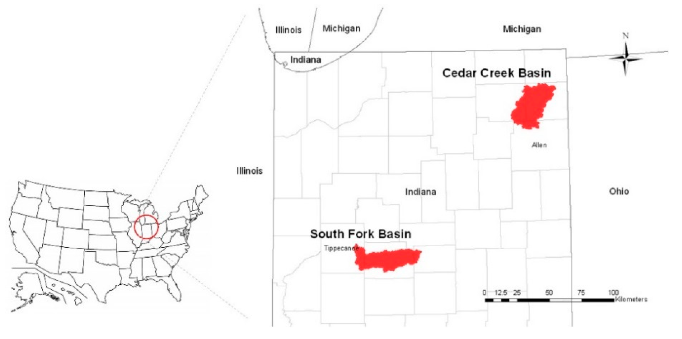
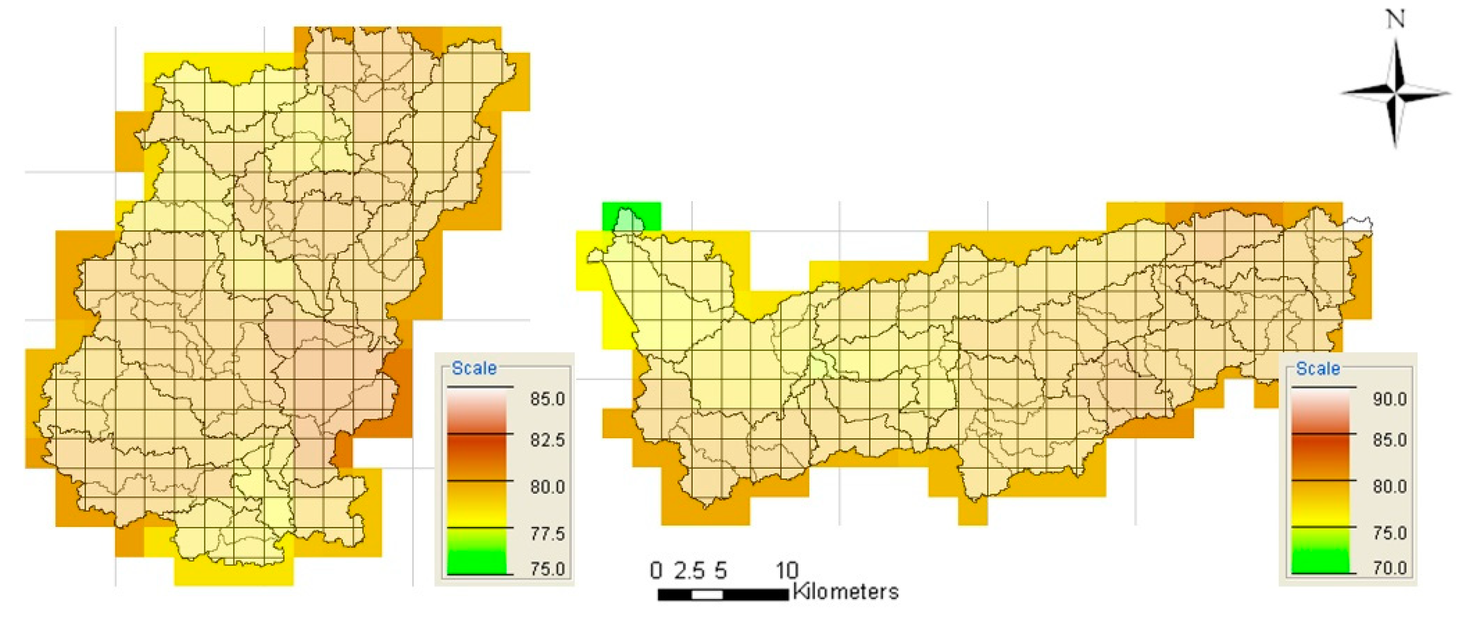
The Cedar Creek and South Fork basins, which are respectively part of the St. Joseph and Wildcat watersheds in U.S., were selected as study sites. These basins are located in Northeastern and Central Indiana State in the USA (Figure 1). The Cedar Creek basin drains an area of 699.30 km2, discharging into the St. Joseph River in Allen County, while the South Fort basin drainage area is 629.37 km2, joining its flow into the Wabash River in Tippecanoe County. For land uses, the Cedar Creek basin predominantly includes crops (58.0%), followed by forest (19.5%), developed area (12.5%), and water (10.0%), and the South Fork basin has crops (37.1%), forest (26.1%), developed area (25.1%), and water (11.7%). The hydrologic soil groups of the Cedar Creek basin are A (4.5%), B (24.7%), C (69.1%), and D (1.7%), and the South Fork Basin has A (0.1%), B (65.1%), and C (34.6%), and D (0.2%), respectively. Accordingly, the average values of Soil Conservation Service (SCS) curve number (CN) [30] for these two basins are 78.57 (Cedar Creek) and 79.60 (South fork) as shown in Figure 2.
2.2. Data
2.2.1. Radar-Based QPEs
The NEXRAD Stage III data (Multi-sensor Precipitation Estimator, MPE), which are corrected with multiple surface rain gauges and have a significant degree of meteorological quality control by trained personnel at individual River Forecast Centers (RFCs) [26,31], were used for this study. Further, from many types of data for this level of radar rainfall (XMRG, netCDF, GIF, DAA, etc., formats), XMRG was selected due to its well-defined data format compared to others; it is typically used for the HEC-GeoHMS applications. XMRG is a binary file used to store gridded data by NWS, and it adopts the Hydrologic Rainfall Analysis Project (HRAP) coordinate system which is defined in a polar stereographic map projection with 4 km by 4 km grid spacing, using a spherical earth datum [25]. These XMRG hourly data are available at the NOAA Hydrologic Data Systems Group (NHDS) and RFC websites [1]. Typically, monthly archives are available for download and can be decompressed to hourly files. The hourly files have a filename convention of: xmrgMMDDYYYYHHz. The HH shown in the filename is the time at the end of the hour of interest.
The XMRG files contain the hourly precipitation estimates on an HRAP grid generated by MPE and Stage III, and they are written row by row from within a ‘do-loop’ using a FORTRAN unformatted write statement. More specifically, the FORTRAN unformatted records have a 4-byte integer (hexadecimal type; F4 10 00 00) at the beginning and end of each record that is equal to the number of 4-byte words contained in the record. The loop is from 1 to MAXY which places the southernmost row as the first row of the file. Additionally, each file consists of two record headers followed by the data. The first and second records of the header contain the contents of the following Table 1 and Table 2.
On the other hand, the precipitation data values are written to the file as integer*2 values (can hold values only up to approximately 32,000; 12 inches) in units of hundredths of mm. Data values for bins which have no radar coverage are set to −1. There are MAXY rows of data each with MAXX values. More detailed information on the XMRG file format can be found on the NOAA website [32].
2.2.2. Gauged Data
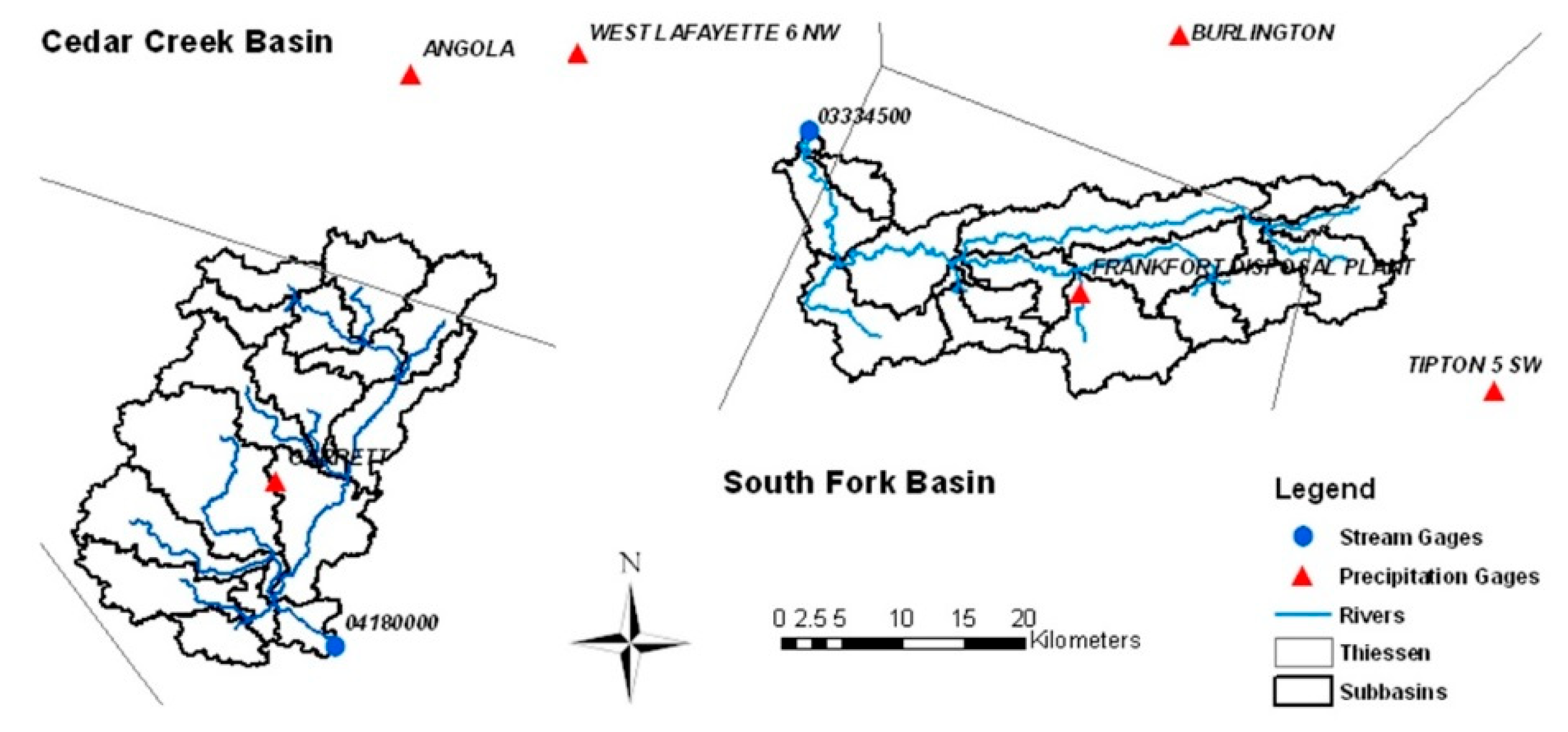
For the Cedar Creek and South Fork basins, only a few (two and four) rainfall gauges were respectively considered with Thiessen polygon to estimate averaged precipitation amounts over the study areas. This is due to the hourly data availability for matching with radar-based data (i.e., NEXRAD Stage III) usaged for hydrologic applications in the following steps. Figure 3 shows the Thiessen polygon included rainfall gauge locations with basin outlets for streamflow observations.
2.2.3. Land Surface Data
The land surface data used in this research are (1) the arc-second digital elevation model (DEM) and National Land Cover Database (NLCD) 2011 from the USGS National Map [33] and (2) the Soil Survey Geographic (SSURGO) database of the USDA Web Soil Survey [34]. These are used for the HEC-HMS model development with curve number map creation.
2.3. Methods
2.3.1. Radar Rainfall Data Processing
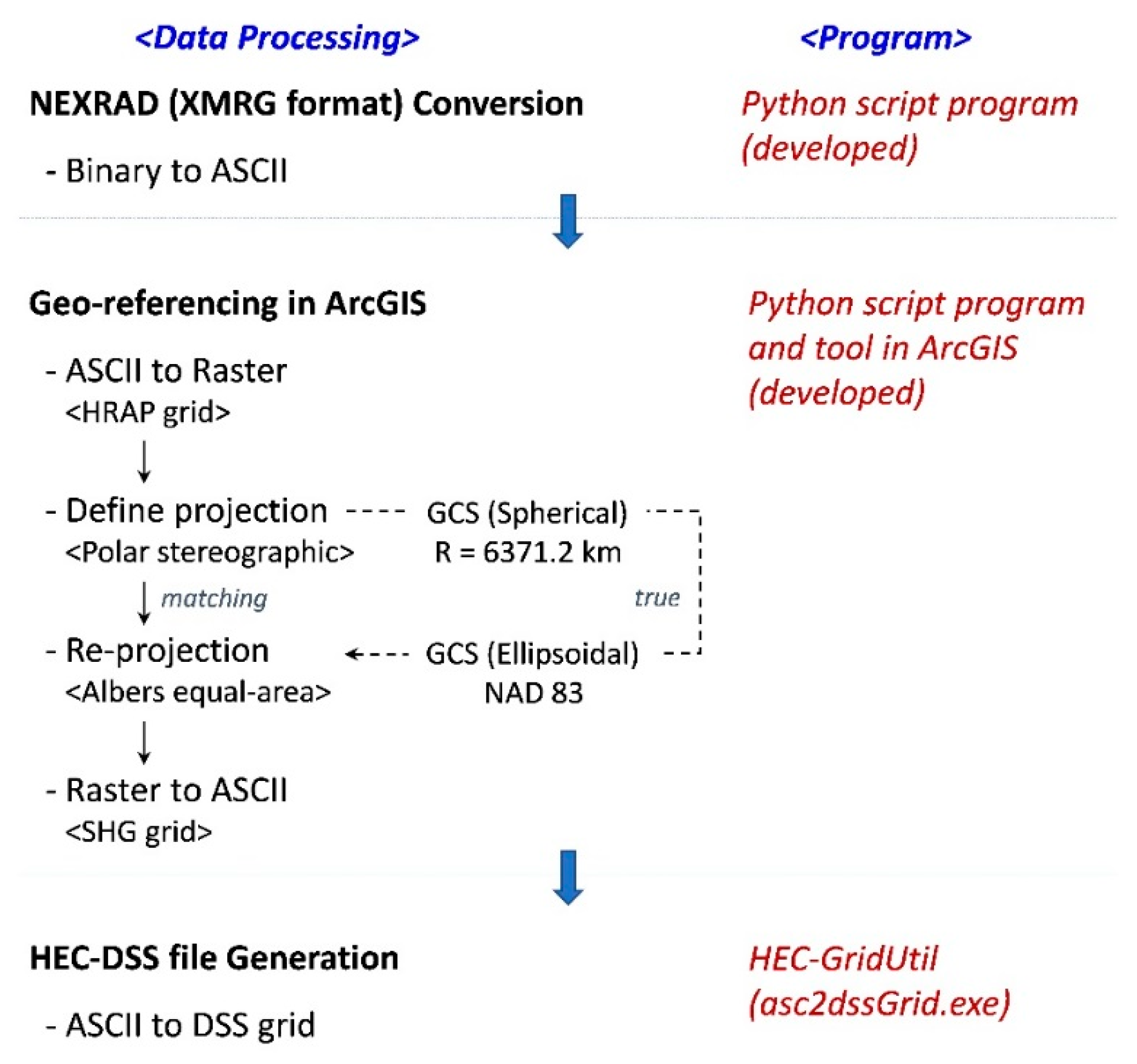
Three steps of radar rainfall data processing were conducted with two main Python script program developments: (1) conversion of the XMRG format (Binary to ASCII) files using a developed Python script program; (2) geo-referencing (re-projection) in ArcGIS using a developed Python script program and geoprocessing tools for GIS application; and (3) DSS file generation using HEC-GridUtil. Figure 4 represents the schematic diagram of radar rainfall data processing. Among these processes, the third processing step utilized an already existing program, since the DSS file for the HEC-HMS application can be generated using the HEC-GridUtil only.
- NEXRAD ConversionThe XMRG format radar rainfall data (NEXRAD Stage III MPE) are stored in a binary file as hexadecimal data. The binary file (not human readable) needs to be converted into an ASCII file with the contents (e.g., header and data) interpretation for practical uses and other analyses. The first developed Python script program supports this kind of conversion processing task. Since the radar rainfall adopted the HRAP grid with a polar stereographic map, the binary file must be rewritten in accordance with this projection (it has two options; HRAP or STER) in the ASCII file. The developed program creates a new ASCII file with many unformatted bytes at the beginning and end of each record handle and loop commands for iterating through the data in Python searching for the required contents.
- Geo-referencing in ArcGISBasically, the better the simulation of a hydrologic model, the more concentrated it will be on matching its projection and spatial resolution for associated data. Therefore, the use of multiple tools having a high amount of input and tasks involving raster data analysis in GIS are required. Thus, the ArcPy module was adopted for handling multiple geoprocessing tools (e.g., Project Raster) in ArcGIS; this is the second developed Python script program. For reference, ArcPy (site-package; a library that adds additional functions to Python) provides access for all geoprocessing tools and a wide variety of useful functions and classes for working with GIS data. Thus, using Python scripts can greatly increase the productivity and quality of maps and data [35].For the HEC-HMS application, the previously converted ASCII file (HRAP grid) should be re-projected into the SHG ASCII file. This can be conducted by using multiple geoprocessing tools in ArcGIS with the developed Python script program along with (1) transforming HRAP coordinates into latitude/longitude geocentric coordinates, (2) converting geocentric latitudes to geodetic latitudes using a datum shift from sphere to ellipsoid, and (3) performing datum transformation between ellipsoids if necessary and projecting geodetic coordinates into Albers equal-area conic map projection. However, other script programs usually omit step 2, referred to as the “matching” transformation, while all three steps above are referred as the “true” transformation [25]. For these, ArcPy was imported into the Python script program for automating the conversion (“true” process) into multiple input files.
- DSS File GenerationAs a final stage of the radar rainfall data processing, the DSS file generation was conducted using HEC-GridUtil because the ArcGIS cannot support it directly. The Hydrologic Engineering Center (HEC) has built an importer (i.e., asc2dssGrid.exe) for a handful of these DSS file formats. The utility bridges the gap between raster GIS and grids in DSS with an intermediate ASCII text file [13].This file consists of a six-line header followed by an array of values laid out like an image of the grid. The six header lines are shown in Table 3. This program is executed by entering its name in the Windows or UNIX command prompt. Input and output files and other parameters are specified after the program name. After this job is done, the resulting DSS file can be directly imported to HEC-GridUtil for display and data handling as well as the HEC-HMS model for hydrologic process application.
2.3.2. HEC-HMS Model Development
The HEC-HMS model which can simulate distributed rainfall–runoff was developed. HEC-GeoHMS (with Arc Hydro) was applied to derive the main model frame of HEC-HMS that enables the ModClark method. Fundamentally, the HEC-HMS model applies the ModClark transform, a simple quasi-distributed approach that applies a linear runoff transform to gridded rainfall excess, as a basic method for distributed rainfall–runoff simulations. Besides, another HEC-HMS model was also developed with the SCS Unit Hydrograph transform method, which can be applied for gauged rainfall data [11]. Eventually, four HEC-HMS models were built with particular transform methods for each study basin, respectively, taking two different stream definition-based sub-basins (one has a 3% threshold of its basin area and the other a 1% threshold) in order to test the model performance against the number of sub-basins (grid cell) as well as to evaluate various simulation results for the selected study sites.
2.3.3. Storm Event Simulation and Evaluation
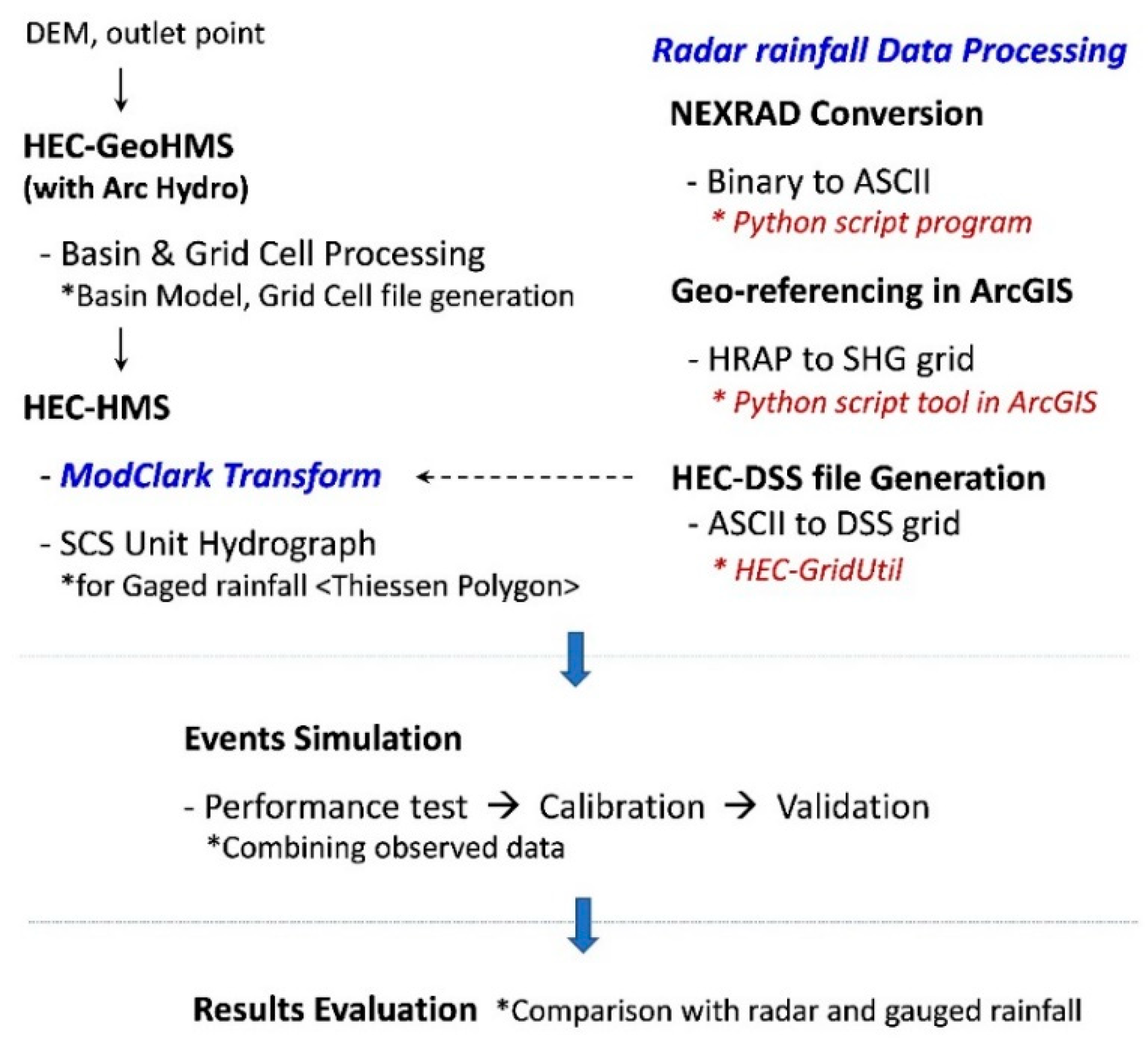
Rainfall data for storms that occurred on 3–10 March 2004, 28 May 2004–7 June 2004, and 26 July 2005–3 August 2005 (radar data—NEXRAD Stage III MPE products) were used for the application of the Modified Clark (ModClark) and SCS Unit Hydrograph (SCS UH) transform methods in HEC-HMS. The radar rainfall data processing, which is converting the data format and generating usable data for the HEC-HMS model execution, was conducted as well. Then event simulations for study areas including model performance tests, calibration, and validation were conducted with evaluation results comparing the radar and gauged rainfall data simulations. Figure 5 represents the schematic diagram of the overall application procedures and methods for this study.
Among the three selected storm events, the first two were used for model performance tests and calibration, and the third was used for model validation. To evaluate the application results, two simple statistics with Nash–Sutcliff efficiency coefficient (ENS) and root mean square error (RMSE) were used, as respectively defined in Equations (1) and (2) below:
where is the measured flow (m3/s), is the simulated flow (m3/s), and is the mean measured flow (m3/s), respectively.
3. Results and Discussion
3.1. Radar Rainfall Data
3.1.1. Processed Data
For the selected storm events, the first data processing for NEXRAD conversion was performed. The processed file name of this step is “ascii_MMDDYYYYHHz.asc”, which is an ASCII file for the HRAP grid. The second step (geo-referencing in ArcGIS) of data processing turns the previous step’s HRAP grid into an SHG grid the file name of which is “shg_MMDDYYYYHHz.asc”. These two grids have different map projections (coordinate systems); thus, the results of these conversions show different view extents with the same dataset in GIS map. Lastly, the DSS file generation (third step) was also processed with a batch file (asc2dssGrid.bat). The resulting format of the generated file from this step returns to a binary file from ASCII with the name of “xmrg_MMDDYYYYHHz.dss”. From these processed individual files (i.e., *.dss file), time-series rainfall input data can be developed using HEC-GridUtil for HEC-HMS flow simulations. For more practical support to utilize these developed programs for radar rainfall data processing, the developed Python scripts, HEC-GridUtil, example datasets, etc., are provided on the GitHub website [36] as Supplementary Materials; Appendix A shows a detailed structural table of these materials.
3.1.2. Amounts and Spatial Variability
Table 4 shows the total areal average rainfall amounts from (1) NEXRAD radar-based data and (2) rain gauge observations (see Figure 3) for the selected storm events over the Cedar Creek and South Fork basins. In case of in-situ rain gauge data, Thiessen polygon weights were calculated to estimate areal average amounts of rainfall storms. As shown in Table 4, some differences can be identified between these two rainfall data sets. These are possibly due to the spatial variability of rainfall amounts, weighting method of gauged data, accuracy of radar-based rainfall estimation, and associated data processing procedures [3,8].
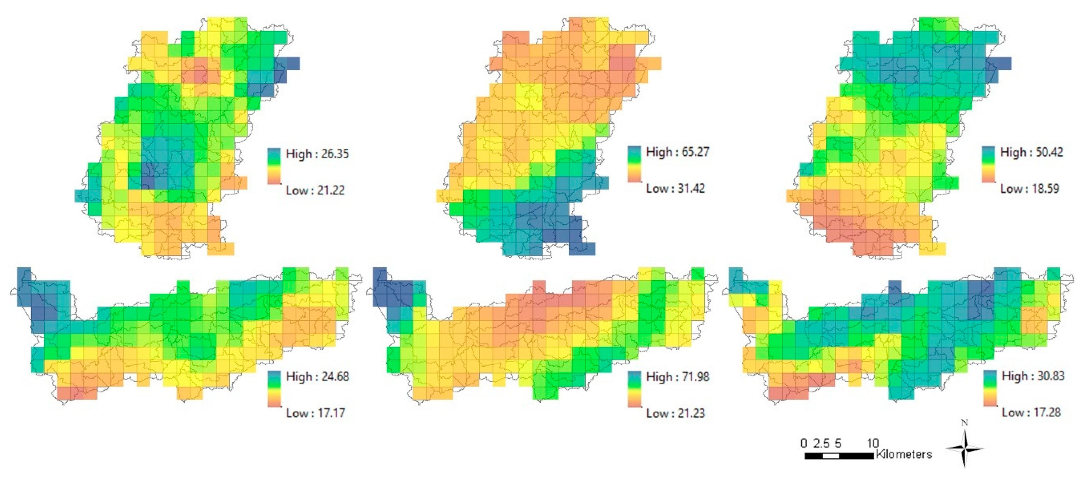
Figure 6 shows the spatial variability of radar rainfall data (cumulative precipitation depth) for the selected three storm events. The spatial distributions using approximately 4 × 4 km SHG grid-based NEXRAD Stage III MPE, which adopt the Albers equal-area conic map projection system, can be seen with each event’s gridded rainfall amounts. For instance, large differences of 171% (18.59–50.42 mm) and 239% (21.23–71.98 mm) occurred in events #3 and #2 for the Cedar Creek and South Fork basins, respectively.
3.2. Model Development
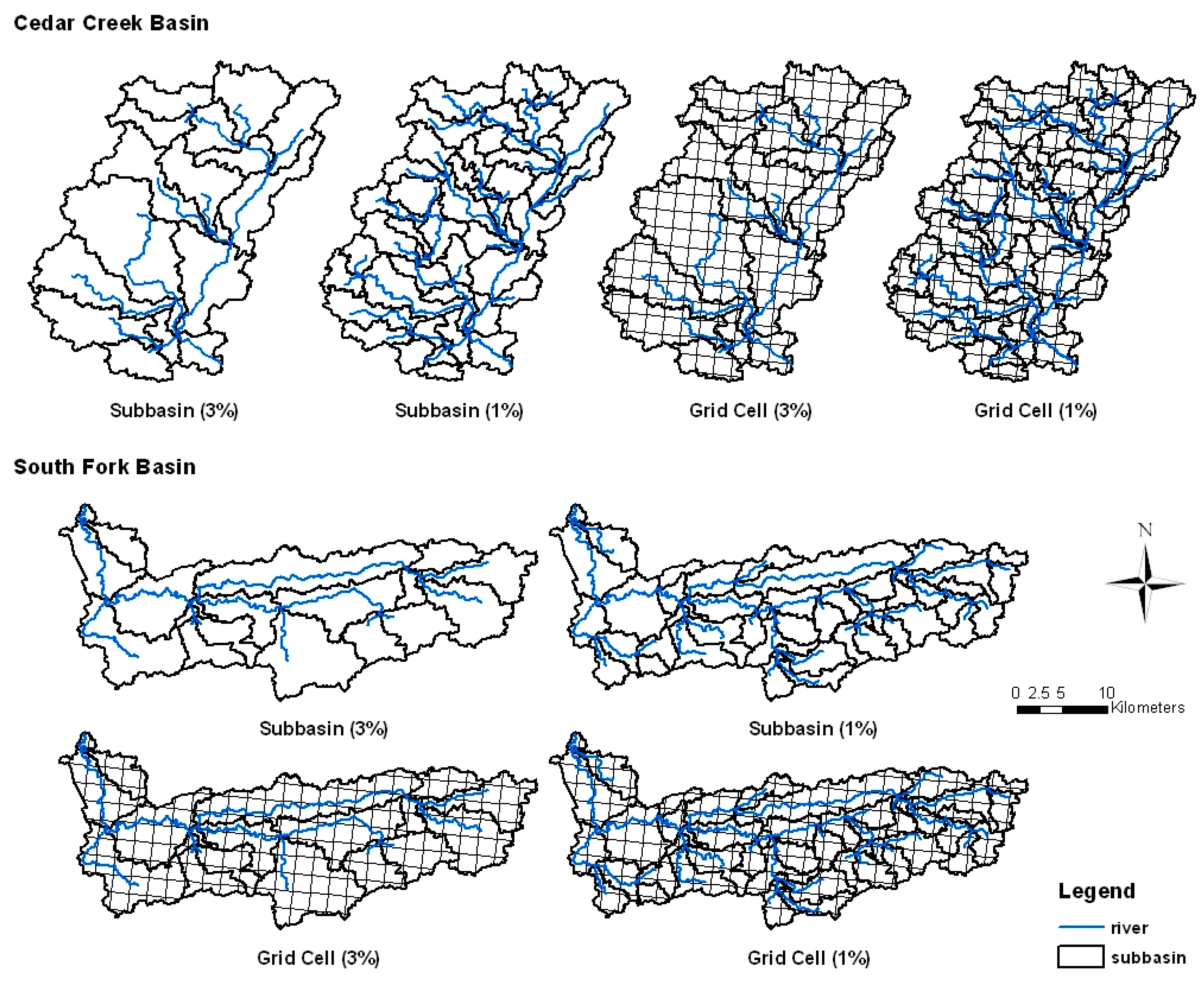
For a total eight developed models of two study basins, the Cedar Creek basin (699.30 km2) was divided into 18 and 52 sub-basins, and the South Fork basin (629.37 km2) was divided into 19 and 50 sub-basins as shown in Figure 7. The number of sub-basins (grid cells), reaches, and junctions for each model are listed in Table 5.
3.3. Model Performance
Three selected storm event-based scenarios for four different HEC-HMS models (i.e., ModClark and SCS UH transform methods adopted 3% and 1% thresholds) of each study basin were implemented; two were used for model performance tests and calibration, and the third was utilized for model validation.
3.3.1. Performance Test
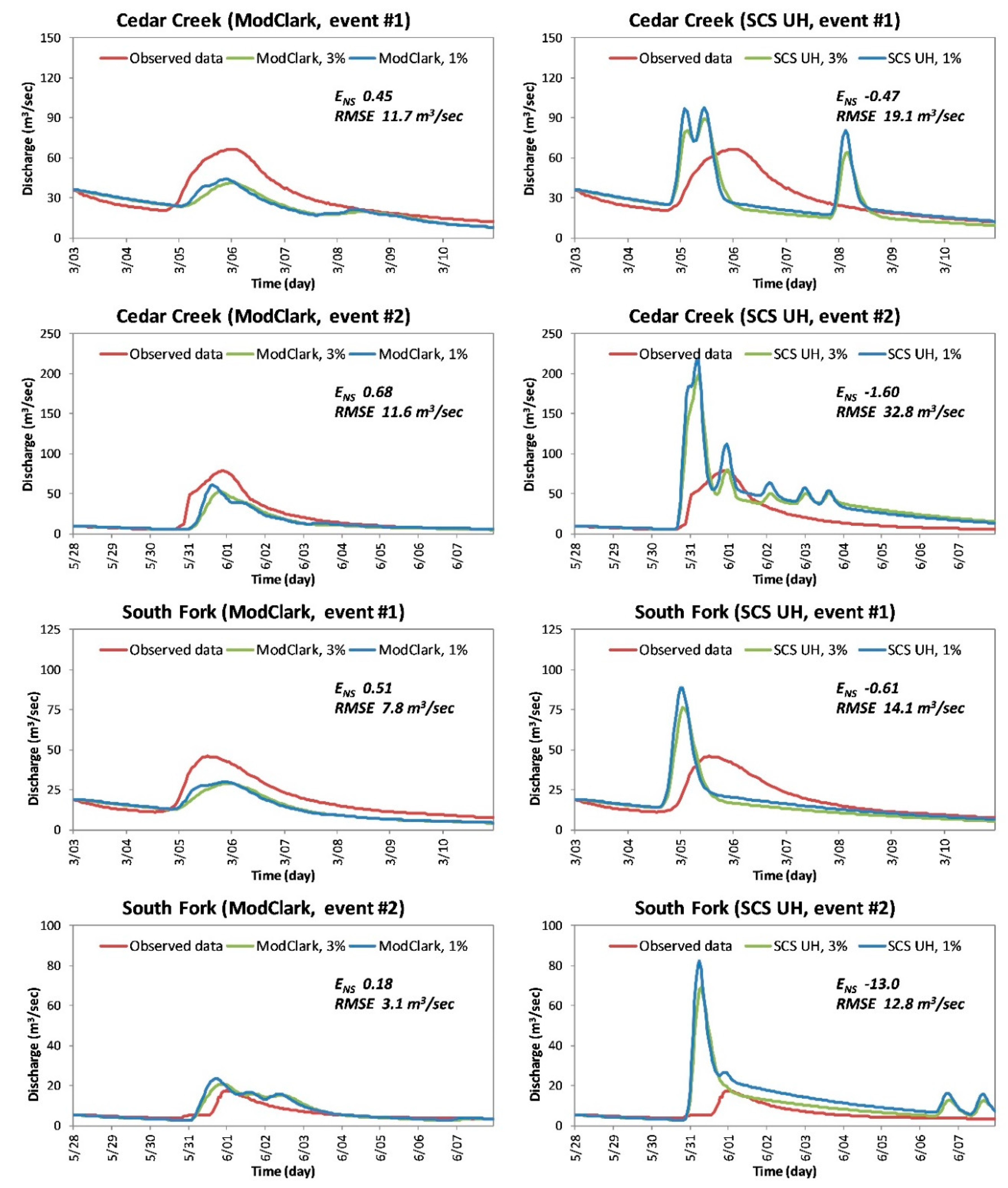
Two storm events (#1 and #2) were tested for the model performance simulations using initial parameter values of both ModClark and SCS UH methods. Typically, HEC-HMS model parameters of loss and baseflow processes are related to the amount of rainfall–runoff and those of transform and river routing are related to the timing of the rainfall–runoff. Among these parameters, basically, the same values of baseflow and river routing are used for both models. However, parameter values of loss and transform are differently launched according to its developed methods; in case of ModClark, it used the gridded SCS CN. Table 6 provides these initial parameter values for the model performance test.
As a part of the model performance test results, Figure 10 compares the storm event #1′s runoff flow hydrographs in South Fork for different numbers of sub-basins which were divided by stream definition. These show slight but not substantial differences affecting the overall model simulation results, representing a slightly slow response to flow in the models with a small number of sub-basins.
For the simulation results of different HEC-HMS models with initial parameter sets in Figure 11, each case of both transform method-based models (i.e., ModClark and SCS UH) did not show perfect fit performances. However, in the ModClark cases using radar rainfall data, it was found that the peak time of simulated streamflow closely matches the peak time of the observed data, whereas the SCS UH cases using gauged rainfall need to shift the time to peak and reduce the flow amount. The results of the statistical analyses for ModClark are superior to SCS UH with ENS values of 0.18 to 0.68 and −13.0 to −0.47, respectively (optimal value 1.0). It seems that the initial model simulations are inadequate.
3.3.2. Calibration
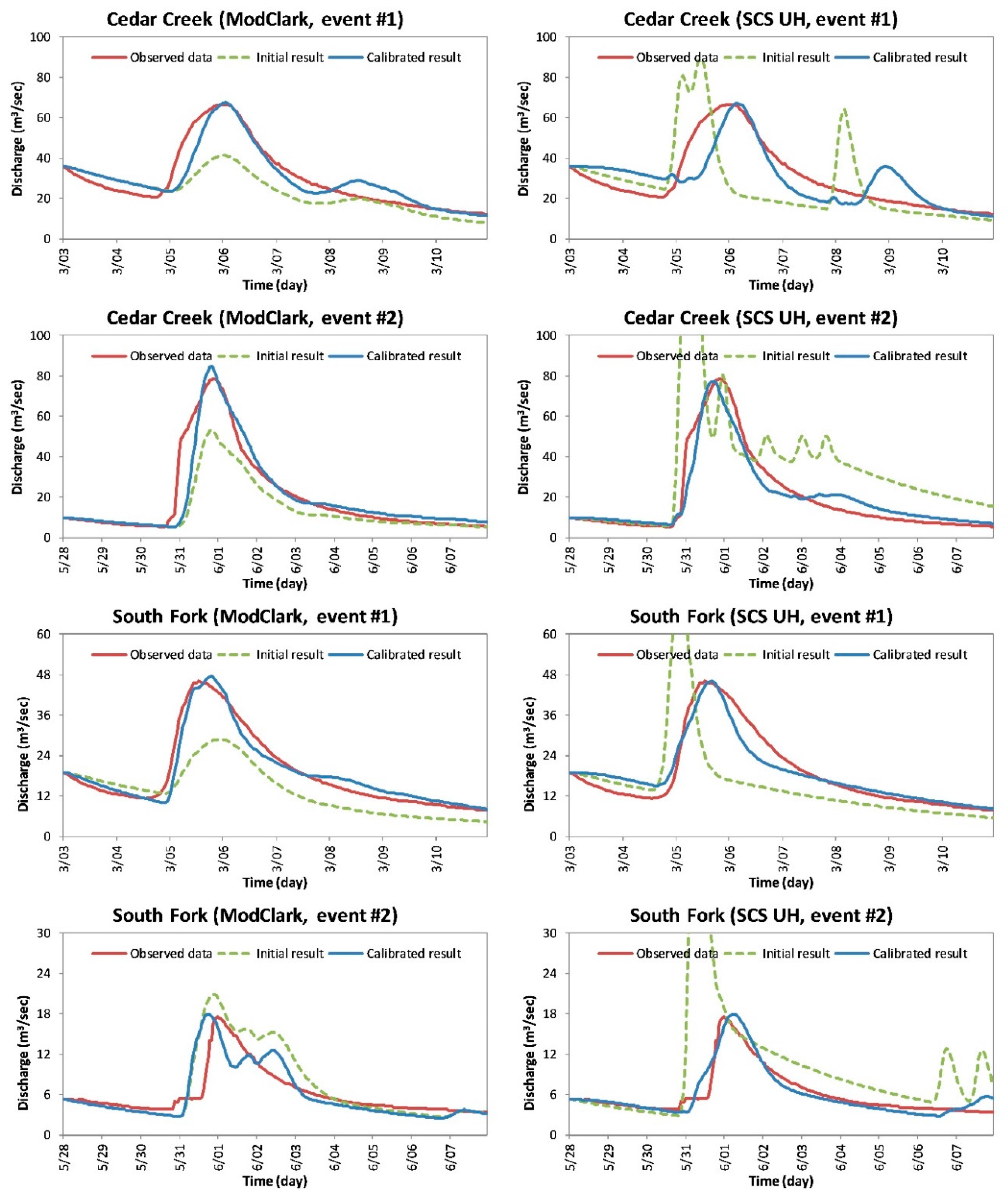
Since the previous model performance test results for different numbers of sub-basins (3% and 1% cases) did not show many substantial differences affecting model outputs, the model calibration was conducted based on the 3% sub-basin models only. For model calibration, total amounts of flow were matched against observations for the same storm events that were used in the initial model performance test. Table 7 includes the calibrated parameter values, and Figure 12 represents the calibrated hydrographs for each model.
The calibration results of the ModClark simulation method using radar rainfall data show relatively good fits with the initial parameter values, but the parameter values of loss factor, baseflow (only one case), and the transform storage coefficient in the South Fork basin for both storm events need to be adjusted. However, there are no parameters to be calibrated for river routing, which are related to the flow timing at the reach level. The other cases for SCS UH method, all the parameter values except transform lag time were adjusted, including the SCS CN initial abstraction, baseflow ratio to peak, and Muskingum routing coefficient (K and X; for hydrograph shifting and attenuation).
In this calibration, only one value for all sub-basins together was adjusted (in some cases, it may be necessary to calibrate for each sub-basin, separately). Thus, some alternations for the level of the sub-basin parameters can be allowed. It means calibrated parameters using two event cases do not always give the perfect fit for the validation of other events or forecasts.
3.3.3. Validation
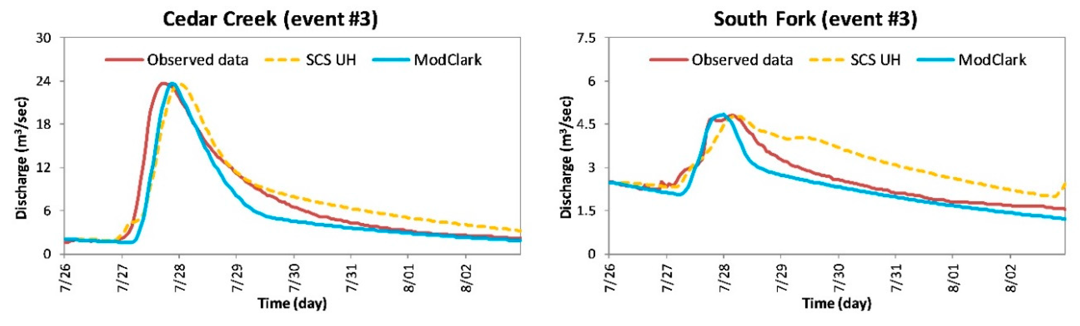
The developed HEC-HMS models’ validation was conducted using the above-mentioned storm event #3. For doing this, the averaged parameter values were used as shown in Table 7, taking into account the calibrated parameter values except loss and baseflow (related to amounts of rainfall–runoff; these parameter values are separately assigned) because they depend on the conditions of the selected events. The results show statistical evaluation values are relatively high when the validation results are compared with the two calibrated models; ENS 0.95–0.98 for ModClark and 0.93 for SCS UH (Table 8 and Figure 13). Thus, both calibrated models can be used for other runoff event flow simulations.
Figure 12 and Figure 13 show the resultant calibration and validation of radar-based and basin-averaged rainfall simulation flows. Both simulated hydrographs using two different methods (i.e., ModClark and SCS UH) provide a reasonable fit to the observed hydrographs. However, the Modclark method-adopted model simulations represent a slightly better fit, having an interesting benefit of no need for adjustments of the parameter values for river reach routing. It reflects the spatial distributions of the radar-observed rainfall for each sub-basin and clearly captures the events for the flow simulation in HEC-HMS with less transform and river routing parameter value adjustments for calibration. In addition, the differences would be due to both the grid-based calculation of losses and the grid-based translation of rainfall excess in the ModClark application.
Although the volume of the basin-averaged rainfall simulation can be adjusted to the observed volume, the shape cannot be matched through only loss rate adjustments. This means the basin-averaged rainfall simulation model using the sparse gauge network around two study basins did not capture this locally intense rainfall activity. Thus, the ModClark method using radar rainfall data is better able to model the spatially distributed nature of these particular events.
The use of radar-based rainfall data for runoff flow simulation has the potential to make major improvements to the modeling of spatially varied rainfall events. Since the localized intensities of convective storms are often missed or not entirely captured by a rain gauge network, radar-based measurements of precipitation which provide for complete spatial coverage of the rain field over a basin are required in the field of flood hydrologic applications. Through the ModClark method in HEC-HMS, these localized rainfall cells can be translated to runoff at the basin outlet. This method is especially useful for areas with poor or non-existent rain gauge coverage where the radar-based rainfall observations have been implemented. The actual run-time for a ModClark model is relatively small, depending on basin size, length of simulation, and traffic on the server [14]. A major drive behind the implementation of ModClark is the improved representation of the spatial and temporal rainfall distributions by NEXRAD. Precipitation input from NEXRAD radar should be more closely aligned with the reality of basin-averaged gauged data. The ModClark method has significant potential for improving forecasting capability when the accurate radar rainfall are used adequately [15].
4. Summary and Conclusions
Throughout this research, three steps of radar rainfall data processing (i.e., NEXRAD Stage III MPE) were conducted for the HEC-HMS applications of rainfall–runoff flow simulation. Two ArcPy-based Python script programs were developed for radar rainfall data type conversion (xmrgtoasc.py) and data map projections (hraptoshg.py). Processed data from a set of developed programs performed well with existing programs (HEC-GridUtil and -HMS). The radar-based rainfall–runoff simulation obtaining hydrographs for comparison with the observed streamflow produced good outcomes. These can reduce the difficulties of radar rainfall data processing and provide efficiency for the HEC-HMS hydrologic process application in spatially distributed rainfall–runoff simulations. After that, eight HEC-HMS models were developed for spatially distributed radar rainfall–runoff (ModClark) and spatially lumped gauged rainfall–runoff (SCS UH) simulations, especially focused on the development of radar-based rainfall data utilized in the runoff flow simulation model. Three event simulations including model performance tests, calibration, and validation were conducted, comparing both method-based models.
For the initial model performance, the simulation results of the ModClark model with radar rainfall data are superior to SCS Unit Hydrograph with gauged rainfall data, and simulation results for different numbers of sub-basins in HEC-HMS did not affect rainfall–runoff flow output strongly. Further, it was found that the spatially distributed radar-based rainfall–runoff simulations show fewer requirements to calibrate the model parameter values; it represents the observed streamflow trend well with the initial parameter sets. For a validation of the results with the calibrated parameters, both models have relatively high statistical evaluation values (ENS 0.95–0.98 for ModClark and 0.93 for SCS UH), but the ModClark method showed a better fit. Therefore, it can be concluded that spatially distributed rainfall–runoff simulations using radar-based rainfall data provide better performances for event simulations than those of gauged rainfall data, but more work remains on the sub-basin level of parameter calibration with separate values.
Since this study was mainly intended to provide comprehensive program developments using Python in ArcGIS (i.e., ArcPy) and their practical application procedures for the radar-based rainfall data processing capabilities, only few storm events (i.e., three cases) in HEC-HMS were provided with simple statistics to evaluate the model’s simulation results. This paper provided methods and programs [36] which are probably useful for users of the HEC-HMS model with data processing to get feasible gridded rainfall inputs because the transfer of radar data to HEC-DSS format is an important aspect of the ModClark modeling process.
Fortunately, as improved radar-based rainfall products as well as satellite-based precipitation estimations [37,38] become available, they can be utilized in the current ModClark capability with modifications or with the newly developed simple hybrid method [7,8] for spatiotemporally distributed hydrological modeling processes. Thus, the method developed in this research can be applied to the different gridded rainfall datasets as well with the same data processing procedures.
Supplementary Materials
The developed Python scripts, HEC-GridUtil, example datasets, etc., are available online at https://github.com/wateryhcho/NEXRAD_ArcPy.
Funding
This research received no external funding.
Acknowledgments
Support for this study (part of Ph.D. course work—term project reports) from Korea Water Resources Corporation (K-water) is gratefully acknowledged.
Conflicts of Interest
The author declares no conflict of interest.
Appendix A

Table A1.
Detailed Structural Table of Supplementary Materials.
Table A1.
Detailed Structural Table of Supplementary Materials.
| Directory or File Name | |||
|---|---|---|---|
| Main Title | Root-Directory | 1st Sub-Directory | 2nd Sub-Directory |
| Original_Data | METADATA.txt | ||
| xmrg_File_Format.pdf | |||
| data | xmrg_MMDDYYYYHHz_OH (set of files) | ||
| Processing_and_Analysis_Steps | METADATA.txt | ||
| step1_conversion | xmrgtoasc.py | ||
| XMRGFiles | xmrg_MMDDYYYYHHz_OH, ascii_MMDDYYYYHHz_OH.asc (set of files) | ||
| step2_georeferencing | hraptoshg.py | ||
| HRAPGrid | ascii_MMDDYYYYHHz_OH.asc (set of files) | ||
| SHGGrid | shg_MMDDYYYYHHz_oh.asc, shg_MMDDYYYYHHz_OH.prj (set of files), etc. | ||
| step3_dss_generation | asc2dssGrid.exe | ||
| asc2dssGrid.bat | |||
| input | shg_MMDDYYYYHHz_oh.asc | ||
| output | xmrg_MMDDYYYYHHz_OH.dss | ||
| Final_Analysis_Products | METADATA.txt | ||
| data | xmrg_08032005_23z_OH.dsc, xmrg_08032005_23z_OH.dss | ||
References
- NOAA (National Oceanic and Atmospheric Administration); NWS (National Weather Service); AHPS (Advanced Hydrologic prediction service). Available online: https://water.weather.gov/precip/download.php (accessed on 1 January 2020).
- NOAA NEXRAD Products. Available online: https://catalog.data.gov/dataset/noaa-next-generation-radar-nexrad-products (accessed on 1 January 2020).
- Peters, J.C.; Easton, D.J. Runoff simulation using radar rainfall data. Water Resour. Bull. 1996, 32, 753–760. [Google Scholar] [CrossRef]
- Kull, D.W.; Feldman, A.D. Evolution of Clark’s unit graph method to spatially distributed runoff. J. Hydrol. Eng. 1998, 3, 9–19. [Google Scholar] [CrossRef]
- Michaelides, S. Editorial for special issue “remote sensing of precipitation”. Remote Sens. 2019, 11, 389. [Google Scholar] [CrossRef] [Green Version]
- Knebl, M.R.; Yang, Z.-L.; Hutchison, K.; Maidment, D.R. Regional scale flood modeling using NEXRAD rainfall, GIS, and HEC-HMS/RAS: A case study for the San Antonio River basin summer 2002 storm event. J. Environ. Manag. 2005, 75, 325–336. [Google Scholar] [CrossRef]
- Cho, Y.; Engel, B.A.; Merwade, V.M. A spatially distributed Clark’s unit hydrograph based hybrid hydrologic model (Distributed-Clark). Hydrol. Sci. J. 2018, 63, 1519–1539. [Google Scholar] [CrossRef]
- Cho, Y.; Engel, B.A. NEXRAD quantitative precipitation estimations for hydrologic simulation using a hybrid hydrologic model. J. Hydrometeorol. 2017, 18, 25–47. [Google Scholar] [CrossRef]
- Zhang, Z.; Koren, V.; Smith, M.; Reed, S.; Wang, D. Use of next generation weather radar data and basin disaggregation to improve continuous hydrograph simulations. J. Hydrol. Eng. 2004, 9, 103–115. [Google Scholar] [CrossRef] [Green Version]
- Scharffenberg, B.; Bartles, M.; Braurer, T.; Fleming, M.; Karlovits, G. Hydrologic Modeling System HEC-HMS User’s Manual; Version 4.3; U.S. Army Corps of Engineers Institute for Water Resources Hydrologic Engineering Center (CEIWR-HEC): Davis, CA, USA, 2018; pp. 1–624. [Google Scholar]
- Fleming, M.J.; Doan, J.H. HEC-GeoHMS Geospatial Hydrologic Modeling Extension User’s Manual; Version 10.1; U.S. Army Corps of Engineers Institute for Water Resources Hydrologic Engineering Center (HEC): Davis, CA, USA, 2013; pp. 1–193. [Google Scholar]
- CEIWR-HEC. HEC-DSSVue HEC Data Storage System Visual Utility Engine User’s Manual; Version 2.0; U.S. Army Corps of Engineers Institute for Water Resources Hydrologic Engineering Center (HEC): Davis, CA, USA, 2009; pp. 1–490. [Google Scholar]
- Steissberg, T.E.; McPherson, M.M. HEC-GridUtil Grid Utility Program Managing Gridded Data with HEC-DSS User’s Manual; Version 2.0; U.S. Army Corps of Engineers Institute for Water Resources Hydrologic Engineering Center (HEC): Davis, CA, USA, 2011; pp. 1–124. [Google Scholar]
- Kull, D.; Nicolini, T.; Peters, J.; Feldman, A. A Pilot Application of Weather Radar-Based Runoff Forecasting, Salt River Basin, MO; U.S. Army Corps of Engineers Institute for Water Resources Hydrologic Engineering Center (HEC): Davis, CA, USA, 1996; pp. 1–32. [Google Scholar]
- CEIWR-HEC. ModClark Model Development for the Muskingum River Basin, OH; U.S. Army Corps of Engineers Institute for Water Resources Hydrologic Engineering Center (HEC): Davis, CA, USA, 1996; pp. 1–51. [Google Scholar]
- Clark, C.O. Storage and the unit hydrograph. Trans. Am. Soc. Civ. Eng. 1945, 110, 1419–1446. [Google Scholar]
- Sabol, G.V. Clark unit hydrograph and R-parameter estimation. J. Hydraul. Eng. 1988, 114, 103–111. [Google Scholar] [CrossRef]
- Anderson, M.L.; Chen, Z.-Q.; Kavvas, M.L.; Feldman, A. Coupling HEC-HMS with atmospheric models for prediction of watershed runoff. J. Hydrol. Eng. 2002, 7, 312–318. [Google Scholar] [CrossRef]
- Piman, T.; Babel, M.S. Prediction of rainfall-runoff in an ungauged basin: Case study in the mountainous region of Northern Thailand. J. Hydrol. Eng. 2013, 18, 285–296. [Google Scholar] [CrossRef]
- Yoo, C.; Ku, J.; Yoon, J.; Kim, J. Evaluation of error indices of radar rain rate targeting rainfall-runoff analysis. J. Hydrol. Eng. 2016, 21. [Google Scholar] [CrossRef]
- Chitu, Z.; Bogaard, T.; Busuioc, A.; Burcea, S.; Sandrid, I.; Adler, M.-J. Identifying hydrological pre-conditions and rainfall triggers of slope failures at catchment scale for 2014 storm event in the Ialomita Subcarpathians, Romania. Landslides 2017, 14, 419–434. [Google Scholar] [CrossRef]
- Shakti, P.C.; Nakatani, T.; Misumi, R. The role of the spatial distribution of radar rainfall on hydrological modeling for an urbanized river basin in Japan. Water 2019, 11, 1703. [Google Scholar]
- Saleh, F.; Ramaswamy, V.; Georgas, N.; Blumberg, A.F.; Pullen, J. A retrospective streamflow ensemble forecast for an extreme hydrologic event: A case study of Hurricane Irene and on the Hudson River basin. Hydrol. Earth Syst. Sci. 2016, 20, 2649–2667. [Google Scholar] [CrossRef] [Green Version]
- Harris, A.; Rahman, S.; Hossain, F.; Yarborough, L.; Bagtzoglou, A.C.; Easson, G. Satellite-based flood modeling using TRMM-based rainfall products. Sensors 2007, 7, 3416–3427. [Google Scholar] [CrossRef] [Green Version]
- Reed, S.M.; Maidment, D.R. Coordinate transformation for using NEXRAD data in GIS-based hydrologic modeling. J. Hydrol. Eng. 1999, 4, 174–182. [Google Scholar] [CrossRef]
- Xie, H.; Zhou, X.; Vivoni, E.R.; Hendrickx, J.M.H.; Small, E.E. GIS-based NEXRAD Stage III precipitation database: Automated approaches for data processing and visualization. Comput. Geosci. 2005, 31, 65–76. [Google Scholar] [CrossRef]
- Paudel, M.; Nelson, E.J.; Downer, C.W.; Hotchkiss, R. Comparing the capability of distributed and lumped hydrologic models for analyzing the effects of land use change. J. Hydroinform. 2011, 13, 461–473. [Google Scholar] [CrossRef]
- Ghavidelfar, S.; Alvankar, S.R.; Razmkhah, A. Comparison of the lumped and quasi-distributed Clark runoff models in simulating flood hydrographs on a semi-arid watershed. Water Resour. Manag. 2011, 25, 1775–1790. [Google Scholar] [CrossRef]
- Alexakis, D.D.; Grillakis, M.G.; Koutroulis, A.G.; Agapiou, A.; Themistocleous, K.; Tsanis, I.K.; Michaelides, S.; Pashiardis, S.; Demetriou, C.; Aristeidou, K.; et al. GIS and remote sensing techniques for the assessment of land use change impact on flood hydrology: The case study of Yialias basin in Cyprus. Nat. Hazards Earth Syst. Sci. 2014, 14, 413–426. [Google Scholar] [CrossRef] [Green Version]
- Soil Conservation Service (SCS). National Engineering Handbook; Section 4: Hydrology; Soil Conservation Service: Washington, DC, USA, 1985. [Google Scholar]
- NOAA NWS DIMP. Available online: https://www.nws.noaa.gov/oh/hrl/dmip/nexrad.html (accessed on 1 January 2020).
- NOAA (National Oceanic and Atmospheric Administration); NWS (National Weather Service); DIMP2 (Distributed Model Intercomparison Project). Available online: https://www.nws.noaa.gov/oh/hrl/dmip/2/xmrgformat.html (accessed on 1 January 2020).
- USGS National Map. Available online: http://nationalmap.gov/viewer.html (accessed on 1 January 2020).
- USDA Web Soil Survey. Available online: https://websoilsurvey.sc.egov.usda.gov/app/WebSoilSurvey.aspx (accessed on 1 January 2020).
- ESRI Python for ArcGIS. Available online: http://resources.arcgis.com/en/communities/python/ (accessed on 1 January 2020).
- GitHub—The World’s Leading Software Development Platform. Available online: https://github.com (accessed on 1 January 2020).
- Liu, Z.; Ostrenga, D.; Teng, W.; Kempler, S. Tropical rainfall measuring mission (TRMM) precipitation data and services for research and applications. Bull. Am. Meteorol. Soc. 2012, 93, 1317–1325. [Google Scholar] [CrossRef] [Green Version]
- Hou, A.Y.; Kakar, R.K.; Neeck, S.; Azarbarzin, A.A.; Kummerow, C.D.; Kojima, M.; Oki, K.; Nakamura, K.; Iguchi, T. The global precipitation measurement mission. Bull. Am. Meteorol. Soc. 2014, 95, 701–722. [Google Scholar] [CrossRef]
Figure 1.
Location of study areas.

Figure 2.
SCSCN for the Cedar Creek (left) and South Fork (right) basins.

Figure 3.
Rainfall gauge and basin outlet locations.

Figure 4.
Schematic diagram of radar rainfall data processing.

Figure 5.
Schematic diagram of the overall application procedures and methods.

Figure 6.
Spatial variability of cumulative precipitation depth (mm) of selected storm events for two study areas, as obtained by NEXRAD Stage III MPE products.
Figure 6.
Spatial variability of cumulative precipitation depth (mm) of selected storm events for two study areas, as obtained by NEXRAD Stage III MPE products.

Figure 7.
Sub-basins and grid cells for the Cedar Creek and South Fork basins.

Figure 8.
Gridded CN for the Cedar Creek and South Fork basins.

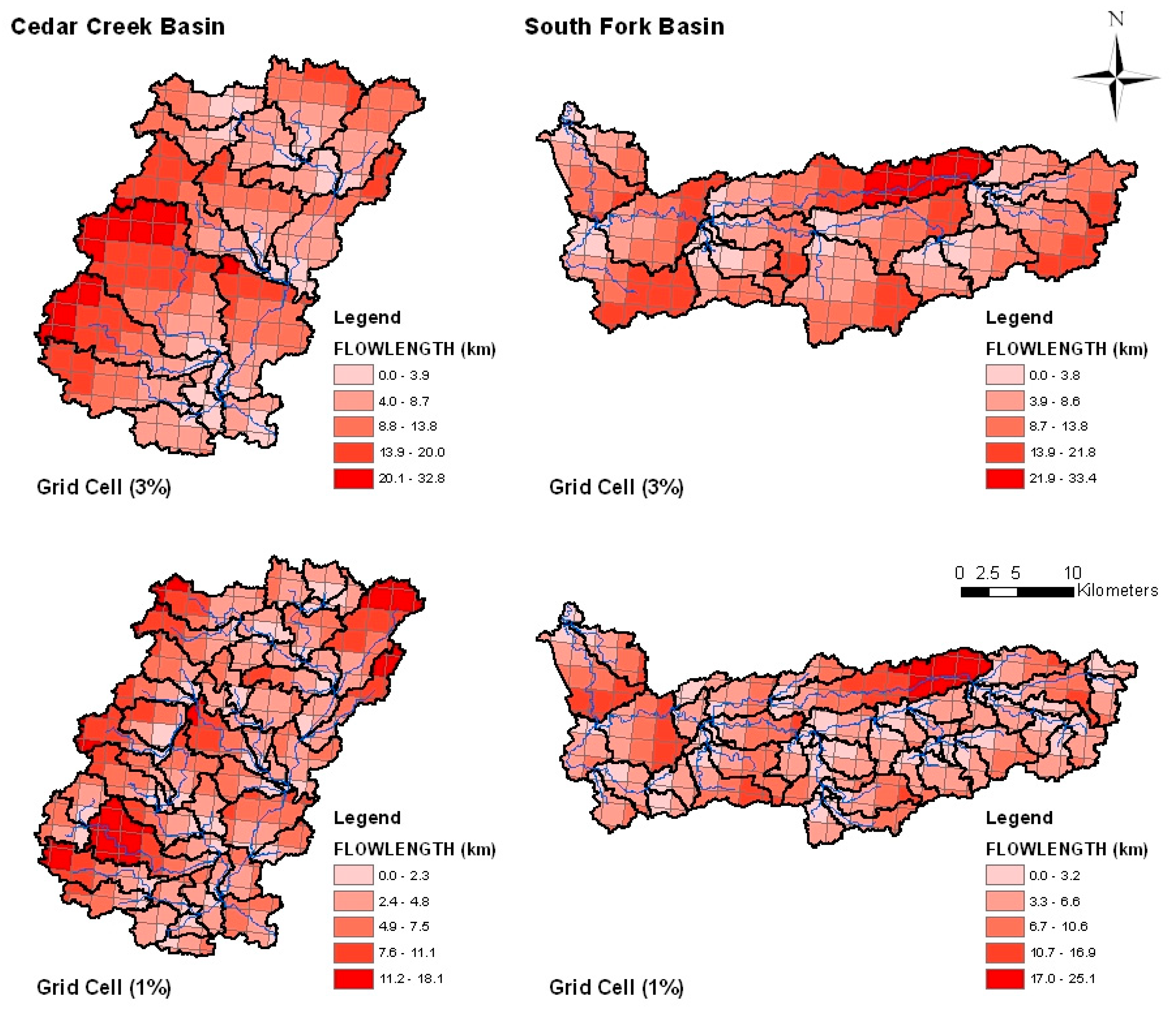
Figure 9.
Flow length of each grid cell for the Cedar Creek and South Fork basins.

Figure 10.
Hydrograph comparisons for models with different numbers of sub-basins.

Figure 11.
Hydrograph comparisons for four different HEC-HMS models.

Figure 12.
Hydrographs for model calibration results.

Figure 13.
Hydrographs for model validation results.

Table 1.
First record of the header for XMRG file.
| Field | Contents |
|---|---|
| 1 | HRAP-X coordinate of southwest corner of grid (XOR) |
| 2 | HRAP-Y coordinate of southwest corner of grid (YOR) |
| 3 | Number of HRAP grid boxes in X direction (MAXX) |
| 4 | Number of HRAP grid boxes in Y direction (MAXY) |
Table 2.
Second record of the header for XMRG file.
| Field | Contents | Type | Details |
|---|---|---|---|
| 0 | oper sys | char*2 | ‘HP’ or ‘LX’ |
| 1 | user id | char*8 | LOGNAME of user that saved the file |
| 2 | saved data/time | char*20 | ccyy-mm-dd hh:mm:ss (Z time) |
| 3 | process flag | char*8 | XXyHH 1 |
| 4 | valid data/time | char*20 | ccyy-mm-dd hh:mm:ss (Z time) |
| 5 | maximum value | integer*4 | In units of millimeters (mm) |
| 6 | version number | real*4 | AWIPS Build number |
1 XX = process code, y = A (automatic) or M (manual), and HH = duration in hours.
Table 3.
Six header lines for the ASCII grid file.
| Name | Description |
|---|---|
| NCOLS | Number of grid columns (integer) |
| NROWS | Number of grid rows (integer) |
| XLLCORNER | Lower left X coordinate (real) |
| YLLCORNER | Lower left Y coordinate (real) |
| CELLSIZE | Cell size (real), this is the width of a square cell. |
| NODATA_VALUE | Value to indicate a null cell, where a value is either missing or has been removed. Default: −9999 |
Table 4.
Total areal average rainfall amounts for the selected storm events.
| Storm Events | Cedar Creek | South Fork | ||
|---|---|---|---|---|
| NEXRAD Radar-Based (mm) | Rain Gauge Observations (mm) | NEXRAD Radar-Based (mm) | Rain Gauge Observations (mm) | |
| #1. 3–10 March 2004 | 23.7 | 27.9 | 20.6 | 20.1 |
| #2. 28 May–7 June 2004 | 45.9 | 46.2 | 38.0 | 25.4 |
| #3. 26 July–3 August 2005 | 34.1 | 31.0 | 25.3 | 29.0 |
Table 5.
Number of sub-basins (grid cells), reach, and junctions for the developed HEC-HMS models.
| Basin | Cedar Creek (SCS UH) | Cedar Creek (ModClark) | South Fork (SCS UH) | South Fork (ModClark) | ||||
|---|---|---|---|---|---|---|---|---|
| Threshold | 3% | 1% | 3% | 1% | 3% | 1% | 3% | 1% |
| Sub-basin (Grid cell) | 18 | 52 | 18 (449) | 52 (612) | 19 | 50 | 19 (391) | 50 (543) |
| Reach | 9 | 26 | 9 | 26 | 9 | 25 | 9 | 25 |
| Junction | 10 | 27 | 10 | 27 | 10 | 26 | 10 | 26 |
Table 6.
Initial parameter values for model performance test.
| Hydrologic Element | Process | Initial Parameter Values | |
|---|---|---|---|
| ModClark (Radar-Based Data Simulation) | SCS UH (Gauged Data Simulation) | ||
| Sub-basin | Loss | Gridded SCS CN - Curve Number grid: determined - Ratio: 0.2 - Factor: 1.0 | SCS CN - Curve Number: determined - Initial abstraction: 0 mm - Impervious: 0% |
| Transform | ModClark - Time of concentration: determined - Storage coefficient: 20 h | SCS UH - Lag Time (min): determined | |
| Baseflow | Recession - Initial discharge (m3/s): observed - Recession constant: 0.8 - Ratio to peak: 0.2 | ||
| Reach | River routing | Muskingum - Muskingum K (hour): 0.5 - Muskingum X: 0.25 - Number of sub-reaches: 1 | |
Table 7.
Calibrated parameter values for each model process.
| Initial Parameter Values | Calibrated Parameter Values | |||||||
|---|---|---|---|---|---|---|---|---|
| Cedar Creek | South Fork | |||||||
| ModClark | SCS UH | ModClark | SCS UH | |||||
| #1 | #2 | #1 | #2 | #1 | #2 | #1 | #2 | |
| Gridded SCS CN/SCS CN | ||||||||
| - Ratio: 0.2/Initial abstraction: 0 mm | - | - | - | 7.87 | - | - | - | 7.11 |
| - Factor: 1.0/Impervious: 0% | 0.20 | 0.65 | - | - | 0.33 | 1.25 | - | - |
| ModClark | ||||||||
| - Time of concentration/Lag time | - | - | - | - | - | - | - | - |
| - Storage coefficient: 20 h | - | - | - | - | 5 | 10 | - | - |
| Recession | ||||||||
| - Initial discharge (m3/s): observed | - | - | - | - | - | - | - | - |
| - Recession constant: 0.8 | - | - | - | - | 0.70 | - | - | - |
| - Ratio to peak: 0.2 | - | - | - | 0.10 | 0.50 | - | 0.28 | - |
| Muskingum | ||||||||
| - Muskingum K (hour): 0.5 | - | - | 6.5 | 4.5 | - | - | 3.5 | 5.0 |
| - Muskingum X: 0.25 | - | - | 0.45 | 0.00 | - | - | - | 0.30 |
| - Number of sub-reaches: 1 | - | - | - | - | - | - | - | - |
Table 8.
Calibrated parameter values for each model process.
| Statistics | Cedar Creek | South Fork | ||||||||||
|---|---|---|---|---|---|---|---|---|---|---|---|---|
| ModClark | SCS UH | ModClark | SCS UH | |||||||||
| #1 | #2 | #3 | #1 | #2 | #3 | #1 | #2 | #3 | #1 | #2 | #3 | |
| ENS | 0.88 | 0.88 | 0.95 | 0.65 | 0.93 | 0.93 | 0.95 | 0.55 | 0.98 | 0.91 | 0.90 | 0.93 |
| RMSE (m3/s) | 5.6 | 7.3 | 2.2 | 9.3 | 5.5 | 2.4 | 2.5 | 2.3 | 0.4 | 3.4 | 1.1 | 0.7 |
© 2020 by the author. Licensee MDPI, Basel, Switzerland. This article is an open access article distributed under the terms and conditions of the Creative Commons Attribution (CC BY) license (http://creativecommons.org/licenses/by/4.0/).
Share and Cite
MDPI and ACS Style
Cho, Y. Application of NEXRAD Radar-Based Quantitative Precipitation Estimations for Hydrologic Simulation Using ArcPy and HEC Software. Water 2020, 12, 273. https://doi.org/10.3390/w12010273
AMA Style
Cho Y. Application of NEXRAD Radar-Based Quantitative Precipitation Estimations for Hydrologic Simulation Using ArcPy and HEC Software. Water. 2020; 12(1):273. https://doi.org/10.3390/w12010273
Chicago/Turabian StyleCho, Younghyun. 2020. "Application of NEXRAD Radar-Based Quantitative Precipitation Estimations for Hydrologic Simulation Using ArcPy and HEC Software" Water 12, no. 1: 273. https://doi.org/10.3390/w12010273
Note that from the first issue of 2016, this journal uses article numbers instead of page numbers. See further details here.