Article

Quantitative Assessment of Specific Vulnerability to Nitrate Pollution of Shallow Alluvial Aquifers by Process-Based and Empirical Approaches

Department of Earth, Environmental and Resource Sciences, University of Naples Federico II, 80126 Naples, Italy
*
Author to whom correspondence should be addressed.
Water 2020, 12(1), 269; https://doi.org/10.3390/w12010269
Submission received: 22 October 2019 / Revised: 7 January 2020 / Accepted: 11 January 2020 / Published: 17 January 2020
(This article belongs to the Section Water Quality and Contamination)

Abstract

:
Shallow aquifers of coastal and internal alluvial plains of developed countries are commonly characterized by the challenging management of groundwater resources due to the intense agricultural and industrial activities that determine a high risk of groundwater contamination. Among the principal origins of pollution in these areas are agricultural practices based on the amendment of soils by nitrate fertilizers, which have been recognized as one of the most severe environmental emergencies for which specific policies and regulations have been issued (e.g., EU Directive 2006/118/EC). In such a framework, the results of research aimed at assessing the specific vulnerability of shallow alluvial aquifers to nitrate fertilizer pollutants by coupled process-based and empirical approaches are here proposed. The research focused on assessing the specific vulnerability to nitrate pollution of a shallow alluvial aquifer of the Campania region (southern Italy), which was selected due to its representativeness to other recurrent hydrogeological settings occurring in alluvial plains of the region and worldwide. In this area, 1D hydro-stratigraphic models of the unsaturated zone were reconstructed and applied for simulating the transport of nitrate pollutants at the water table and estimating the associated travel times. Numerical modeling was carried out by the finite differences VS2TDI code and considered a 10-year time series of rainfall and evapotranspiration as well as typical local farming practices of nitrate fertilizer input. Results of the travel time calculated for the 1D hydro-stratigraphic models considered and at different depths were recognized as a proxy to assess the specific vulnerability to nitrate fertilizer pollution. Among the principal outcomes is an empirical multiple correlation between the travel time of the nitrate fertilizer pollutant, water table depth, and equivalent saturated hydraulic conductivity of the unsaturated zone or hydraulic resistance, which was used to assess the travel time at the distributed scale over the whole area studied as well as the related specific vulnerability. Given such results, the coupled process-based and empirical approach is proposed as generally applicable for assessing and mapping groundwater vulnerability in shallow aquifers, for which detailed stratigraphic and piezometric data are available.

Graphical Abstract

1. Introduction

The environmental impacts of industrial and agricultural activities are the main causes determining the decay of the hydro-chemical quality of groundwater, which represents the most important source of drinking water in developed countries. For this reason, specific policies aimed at the protection and sustainable management of aquifers have been issued, as in the case of Europe with EU Directive 2006/118/EC [1] and European Environment Agency (EEA) [2]. A relevant part of these policies, especially those aimed at the territorial planning and protection of aquifers, have focused on the relevance of assessing and mapping groundwater vulnerability [3,4,5] resulting from anthropic activities.
Groundwater vulnerability is largely considered as the potential level of groundwater contamination, which is controlled by natural attenuation processes occurring in the unsaturated zone, from the source of pollution to the saturated zone of the aquifer [6,7]. Starting from such a conceptual framework and considering processes controlling the migration of pollutants in the unsaturated and saturated zones, groundwater vulnerability depends on three principal process series: (1) the flow velocity of water and fluid pollutants through unsaturated and then saturated zones of the aquifer; (2) residual concentration of fluid pollutants at the groundwater table, which identifies the capacity of the unsaturated zone to attenuate its initial concentration; and (3) decrease in the pollutant concentration in the saturated zone by advective dispersion, diffusion, and geochemical processes.
Considering the variable dependence of attenuation processes in the unsaturated and saturated zones on the type of pollutant, groundwater vulnerability is usually subdivided into intrinsic and specific vulnerability [8]. Intrinsic vulnerability of an aquifer is considered as its capability to receive, convey, and attenuate a generic pollutant through the unsaturated and saturated zone depending on the geological, hydrological, and hydrogeological features of both [9,10]. On the other hand, specific vulnerability is related to specific contaminants by considering their peculiar physical and chemical properties, with the associated attenuation processes occurring in the unsaturated and saturated zones [7].
Since the 1970s, many researchers have developed different methodological approaches for assessing and mapping the intrinsic vulnerability of aquifers [11,12]. More recently, several studies have shown that intrinsic vulnerability maps derived from the application of these methods may result in different or even contrasting assessments, depending on the scales of analysis, hydrogeological parameters, and hydrogeological framework considered [13,14,15].
Methodological approaches used for assessing and mapping the intrinsic vulnerability of aquifers vary roughly in three main groups, depending on the scale of territorial analysis [6]. The first group comprises the hydrogeological complex and settings methods (HCS), which assesses intrinsic vulnerability at the regional scale by heuristic approaches based on qualitative estimates of hydrogeological and geomorphological features [11].
The second group includes the parametric system methods (PS) that estimate the intrinsic vulnerability of aquifers by semi-quantitative approaches based on the identification of hydrogeological, topographic, and land use factors controlling the propagation of pollutants through the unsaturated and saturated zones and the attribution to them of a score dependent on the assumed impact on the aquifer vulnerability. Scores assigned to the different factors are combined by a map overlaying procedure, thus estimating a vulnerability index as the sum of score values. This group of methods includes matrix systems (MS) based on the combination of two parameters; rating systems (RS) consisting of the combination of scores attributed to some parameters; and point count system models (PCSM) based on the combination of scores and weights to some parameters. Examples of methods belonging to these groups include, among others: GOD [4], DRASTIC [12], AVI [16], SINTACS [6,17], DAC [18], ISIS [19], GLA [20], PI [21], and EPIK [22]. Among these methods, the most commonly used is DRASTIC, which has been applied to map the intrinsic vulnerability of aquifers in many parts of the world [23] and whose structure has been developed to create other similar approaches such as SINTACS [6,17]. Moreover, several attempts have been carried out to modify the original DRASTIC structure for assessing the specific vulnerability to nitrate fertilizers [24,25,26,27,28,29] or pesticide pollutants [30].
The above-mentioned two groups of methods express groundwater vulnerability qualitatively through an ordinal scale. The principal points of weakness of these approaches are the uncertainty in the attribution of ratings due to the subjective criteria used, the lack of a real quantitative assessment of groundwater vulnerability, and the impossibility of a direct comparison among the results obtained from different methods.
Even if there is not a generally accepted quantitative indicator to measure groundwater vulnerability [31,32,33], a third group of methods comprises quantitative approaches based on analytical solutions or numerical modeling of pollutant transport through the vadose and saturated zones to be applied on physical models. These approaches allow for the mapping of groundwater vulnerability by combining flow and transport models and infiltration and evapotranspiration rates with a solution to the advection-dispersion equation. Given the need for reliable 3D physical models, thus, a great availability of stratigraphic and hydrogeological data, such methods can be generally applied to local or site-specific scales, for which detailed and expensive investigations are to be carried out. Through these modeling approaches, one of the most used indicators of groundwater vulnerability is the travel time of a pollutant through the unsaturated zone, which is estimated by analytical advective-dispersive transport models [34,35,36,37], variance of the pollutant break through curve at the water table [38], finite element models [39,40] or type transfer functions (TTFs) [41]. The same approaches are used to assess the specific vulnerability of aquifers, considering geochemical and other attenuation processes controlling the transport of a specific pollutant in both the unsaturated and saturated zones. In the case of nitrate fertilizers pollutants, models estimating the losses of nitrogen leaching beneath the root zone and simulating the transport and transformation of nitrogen from agricultural land and soil profiles such as GLEAMS [42,43] and HYDRUS [44], or indices such as LOS [45] have been developed.
The study presented here specifically focused on estimating groundwater vulnerability to the pollution of shallow alluvial aquifers that characterize a large part of the internal and coastal plains of the region, where agricultural and livestock productions have been extensively developed and the groundwater demand is very high, as the risk of groundwater pollution. Among the multiple sources of pollution, farming practices based on the use of nitrate fertilizers represent the major threat for groundwater quality in these areas, especially for shallow alluvial aquifers [46,47,48]. Therefore, this study addressed the estimation of the specific aquifer vulnerability to nitrate fertilizer pollutants of a representative shallow alluvial aquifer in a sector of the Campanian Plain corresponding to the adjoining Casalnuovo di Napoli and Volla municipalities, located along the eastern border of the city of Naples (southern Italy). This aquifer was also considered representative for the anomalous high concentrations of nitrate in groundwater resulting from hydro-chemical studies carried out in the plain area surrounding the city of Naples [46,48].
The goal of the study presented was focused on estimating and mapping specific aquifer vulnerability through the assessment of the travel time of nitrate fertilizer pollutants through the unsaturated zone at the water table [49,50], which is defined hereinafter as the Unsaturated Zone travel Time (UZT). For such a scope, the hydrogeological characteristics of the unsaturated zone as well as the specific hydrological regime of the area were taken into account in the 1D numerical modeling of pollutant transport through the unsaturated zone in different representative hydro-stratigraphic conditions. The results were used to find an empirical relationship linking UZT to water table depth and equivalent hydraulic conductivity of the unsaturated zone. The application of such an empirical model has allowed for the estimation and mapping of groundwater vulnerability at the distributed scale in the study area.

Study Area Description

The study area is located in the eastern plain of Naples (Campania region—southern Italy). It extends over about 14 km2 and corresponds to the adjoining municipalities of Casalnuovo di Napoli and Volla (Figure 1a,b). From a geological point of view, this area belongs to the larger Pliocene structural depression (graben) of the Campanian Plain, which was filled with pyroclastic deposits and lavas erupted by the Phlegraean Fields (60 k-yrs—1538 A.D.) and Mount Somma-Vesuvius (39 k-yrs—1944 A.D.) volcanic centers [51,52]. In addition, during the Plio-Pleistocene period, alluvial, marine, and fluvio-palustrine sediments filled the tectonic depression, forming a pyroclastic-alluvial plain characterized by a high stratigraphic heterogeneity and lateral variability [53,54].
From a hydrogeological point of view, the study area is a sector of the aquifer system of the eastern plain of Naples, whose groundwater circulation can be considered unitary at the regional scale (Figure 1a) [55,56,57]. The conceptual flow model (Figure 1a) shows a general groundwater flow oriented from NE to SW with a main contribution to groundwater recharge deriving from rainfall and lateral groundwater inflows from the adjoining karst aquifers of the southern Apennines and Somma-Vesuvius volcanic aquifer (Figure 1a).
At the local scale (Figure 1b and Figure 2), the study area is characterized by an aquifer system [58]. The northern and central sectors are characterized by a phreatic shallow alluvial aquifer and a deep semi-confined one separated by the Campanian Ignimbrite (CI, 39 k-yrs) tuff [59], which behaves as an aquitard. Instead, the southern sector, corresponding to the ancient Sebeto River Valley (Figure 1 and Figure 2) is characterized by a unique phreatic alluvial aquifer due to the lack of a CI aquitard [58]. This research was focused on the shallow alluvial aquifer extending continuously over the whole study area.
The groundwater circulation, according to the general basin-scale pattern, is oriented from NE to SW (Figure 1a,b) and converges toward the drainage axis corresponding to the Sebeto River Valley and its tributaries (Cozzone and Volla Rivers).
The setting of groundwater circulation is due to the current spatial distribution of piezometric levels that have varied strongly in the last 50 years [58]. During the period between 1950 and 1989, a rapid decline of groundwater levels occurred at the groundwater basin scale due to the overexploitation of groundwater resources for drinking, industrial, and agricultural uses. As an effect of overexploitation, increasingly, deep groundwater has been pumped, causing the decay of its quality due to the rise in nitrates, fluoride, iron, and manganese concentrations beyond the accepted limit for drinking water [60,61]. Therefore, since the beginning of the 1990s, groundwater abstraction for drinking use has been progressively abandoned, causing a groundwater rebound [56] with a rise in piezometric levels in the study area of up to about 16 m, determining the relevant impacts on human activities related to groundwater flooding and ground deformations [58,62,63,64].
The study area presents relevant environmental issues depending on the types of land use, which is characterized by a high diffusion of urbanized areas covering approximately 65% of the territory, and subordinate agricultural practice extended over the rest (35%) (Corine Land Cover, 2012). Accordingly, the strong anthropogenic pressure affects the qualitative state of groundwater. Recent studies [48] have shown that in the three-year period between 2012 and 2015, the nitrate concentrations in groundwater reached values higher than the acceptance limit for drinking water (50 mg/L), with an increasing trend in comparison to the previous three-year period (2008–2011).

2. Data and Methods

2.1. Modeling of Nitrate Pollutant Transport

The specific vulnerability of the studied aquifer to nitrate fertilizer pollution was assessed by the estimation of the unsaturated zone travel time (UZT) of the pollutant at the water table [10,49,50], considering both all the possible hydrogeological conditions existing in the unsaturated zone and modeling its hydrologic response to transporting the pollutant over a 10-year time span.
To achieve this goal, a numerical simulation of the nitrate pollutant transport in the unsaturated zone was carried out by the VS2DTI code [65], which is a physically-based finite differences model for simulating fluid flow and solute or energy transport through variably saturated porous media. Stratigraphic data deriving from geological surveys carried out in the study area were considered to define several representative 1D physical models. These data were obtained by 86 boreholes drilled in the study area, mainly with the scope of geotechnical investigations, which were collected from the archives in the city halls of the Casalnuovo di Napoli and Volla municipalities.
Moreover, a field campaign of piezometric level measurements, carried out in 2013 [58,62,63], was considered for mapping the water table depth. The piezometric network considered was based on 108 wells used for domestic, agricultural, and industrial requirements, with depths varying from 10 to 60 m. The piezometric heads were spatially interpolated by the kriging geostatistical algorithm. In this scope, a double structure variogram was used to interpret the spatial anisotropy [62]: (i) a sferic model along the direction −60°, with range = 1150, sill = 1.55, nugget = 0; (ii) a Gaussian model along the direction 30°, with range = 1780, sill = 3, nugget = 0.
Through a first analysis of the borehole data, principal stratigraphic settings were recognized as mainly formed by typical and complex interfingering between alluvial deposits and pyroclastic soils erupted by the Phlegraean Fields and Somma-Vesuvius Volcanoes and generally characterized by alternating fine to coarse ashes and pumiceous lapilli horizons [54,66]. Starting from these data, 1D representative hydro-stratigraphic models were reconstructed down to the depth of 20 m, considering both homogeneous and heterogeneous stratigraphic conditions, with soil horizons varying in grain size from sand to silt. The limitation to 20 m of the depth considered in modeling was assumed due to typical values of the water table depth occurring in shallow alluvial aquifers of the Campanian Plain.
With regard to the main physical and hydraulic properties of the soil horizons modeled such as saturated hydraulic conductivity (Ksat) and unsaturated properties for the van Genuchten’s [67] parameterization of the soil water retention curves (SWRCs), the VS2DTI catalog of values for generic USDA soil textural classes [68,69] was considered (Table 1).
The upper boundary condition of each model domain includes a vertical flux entering through the ground surface, to which variable daily rainfall and evapotranspiration rates such as periodical surficial pollutant input were assigned. The lateral boundary conditions of the models were set with no flux because only the 1D (vertical) flow was considered with no lateral outflows or inflows. Finally, the bottom boundary condition, corresponding to the water table, was set as a possible seepage face due to the scope of estimating UZT at its depth and to avoid the formation of an unreal saturated zone developing from the bottom of the model domain.
To simulate hydrological conditions controlling the UZT of nitrate pollutants to the water table, the initial soil pressure head distribution of the models was set to match soil hydrological conditions that characterize soils of pyroclastic origin during winter [70]. Time-varying parameters controlling water losses by evapotranspiration including rooting depth (RD), root activity at base (RAB), root activity at top (RAT), and the root pressure head (RPH) were defined according to field observations, type of agricultural practice, and the literature data (Table 2).
As input for the model, the daily rainfall and air temperature time series from September 2003 to August 2013, gathered by regional meteorological network of the Centro Agrometeorologico Regionale (C.A.R.) of the Campania Region, were used to simulate the hydrological response for a 10-year time span (Figure 3). Specifically, the hydrological time series recorded by the Marigliano Meteorological Station, located about 10 km from the study area, were considered. The daily time-scale evapotranspiration rate was estimated using Hargreaves’s equation [71,72]. The time step of the simulations was set equal to 86,400 s (one day).
1D models were provided with 20 observation nodes distributed along the vertical (Figure 4) and positioned every 0.50 m, in the first 10.0 m of depth, and every 1.00 m from 10.0 m to 20.0 m of depth. The output of the model at the observation nodes allowed us to obtain the daily values of soil water content, saturation degree, soil pressure head, and pollutant concentration for all the modeled hydrological years. According to typical local farming practices, a one-day spill per year of nitrate fertilizer was set as an input for every first week of September in the 10-year modeling period. For all the conceptual models considered, four different input concentrations of pollutant were chosen: 1.0, 3.0, 5.0, and 7.0 mg/L.
Finally, hydrodynamic parameters for nitrate pollutants such as the coefficient of molecular diffusion in the porous medium (CMD), and longitudinal-transverse dispersivity (LD and TD, respectively) were defined (Table 2) according to the literature [73,74]. Due to the principal goal of the research, which was focused on assessing specific aquifer vulnerability to nitrate pollutants by estimating UZT and not to calculate the concentrations of pollutants arriving at the water table, the phenomena of nitrate retention by plant absorption in the root zone [43,75,76] and the effects of denitrification process in the unsaturated zone were not taken into account. For this scope, a simple conservative approach was adopted by setting the decay parameter (DC) as “no decay” and thus simulating no geochemical or physical interactions with soil particles or other intra-pore fluids (Table 2). Consequently, the nitrate pollutant was considered conservative, namely characterized by concentrations not reduced by biological or geochemical processes occurring in the unsaturated zone. Such a choice is supported by the results of studies indicating that the reduction of nitrate in the unsaturated zone below the root zone is limited to 1–2% [77,78]. The same simplifying approach has also been used in other studies focused on estimating the UZT of nitrate fertilizer pollutants [28,79].

2.2. Estimation of the Unsaturated Zone travel Time (UZT) of Nitrate Pollutant

The UZT of nitrate pollutants was considered as corresponding to a given value of the relative concentration, namely the ratio between the pollutant concentration in a specific time step of the simulation (Ci), simulated for a given depth, and the initial concentration value at the ground surface (C0). Specifically, the UZT was identified on the pollutant breakthrough curve with the time starting from the nitrate input at the ground surface, at which the condition Ci/C0 ≥ 1% occurs at different depths. This approach is also considered precautionary in comparison to others that have estimated the UZT by the arrival time of 50% [40] or the 75% [80] solute mass breakthrough curve at the groundwater table.
In this way, considering the UZT values calculated for each representative hydro-stratigraphic model at different depths, corresponding to the observation nodes of the models, the relationship with the depth was analyzed.

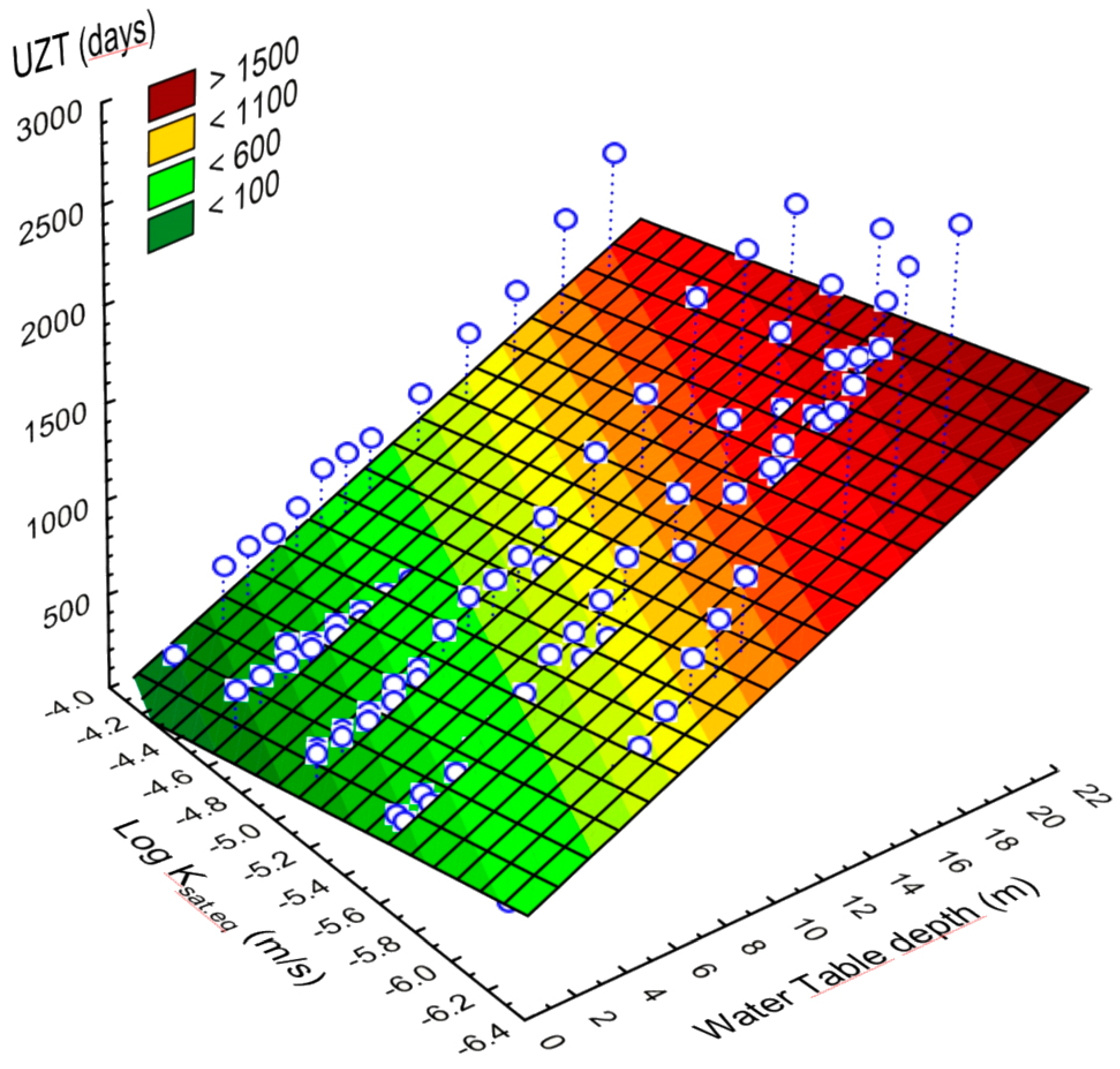
2.3. Generalization of UZT Results at the Distributed Scale

Considering the results of UZT obtained for different representative hydrogeological conditions and at different depths, an attempt to generalize these results from the 1D scale to a distributed one was carried out by an empirical multiple correlation among water table depth (D) and the equivalent saturated hydraulic conductivity (Keq.z) of the unsaturated zone, estimated in the vertical direction and perpendicularly to the layering, or hydraulic resistance of the unsaturated zone [29], calculated by the following formula [81]:
K eq . z   =   D i = 1 n h i K sat . i
where D = depth to water table; n = number of hydro-stratigraphic horizons; hi = thickness of the ith hydro-stratigraphic horizon; and Ksat.i = saturated hydraulic conductivity of the ith hydro-stratigraphic horizon.
To use such an empirical relationship for the assessment of UZT at the distributed scale, raster maps, with a resolution of 5 × 5 m, of water table depth (D) and equivalent saturated hydraulic conductivity (Keq.z) of the unsaturated zone, were reconstructed. At this scope, a map of water table depth was calculated as difference between the digital terrain model (DTM), derived from the LiDAR dataset, and the map of piezometric heads, derived from the spatial interpolation of piezometric head measurements carried out in 2013 by a field campaign [58,62].
Moreover, given the availability of stratigraphic data derived from 86 boreholes and considering that stratigraphic columns resulted as formed prevailingly by soil material with known grain size mixtures, an estimate of saturated hydraulic conductivity (Ksat) was carried out for each stratigraphic soil horizon by the VS2DTI catalog, which is based on generic USDA soil textural classes [68,69]. Using this approach, stratigraphic columns were transformed in logs of Ksat, then Keq.z was calculated with the preceding equation (Equation (1)). Subsequently, values of Keq.z, estimated for each borehole, were spatially interpolated by the kriging interpolation, obtaining a raster map of Keq.z for the studied area.
Finally, given the availability of the map of water table depth (D) and of the equivalent saturated hydraulic conductivity along the vertical (Keq.z) as well as of the empirical relationship linking both variables, the UZT map for nitrate pollutant was calculated.

3. Results

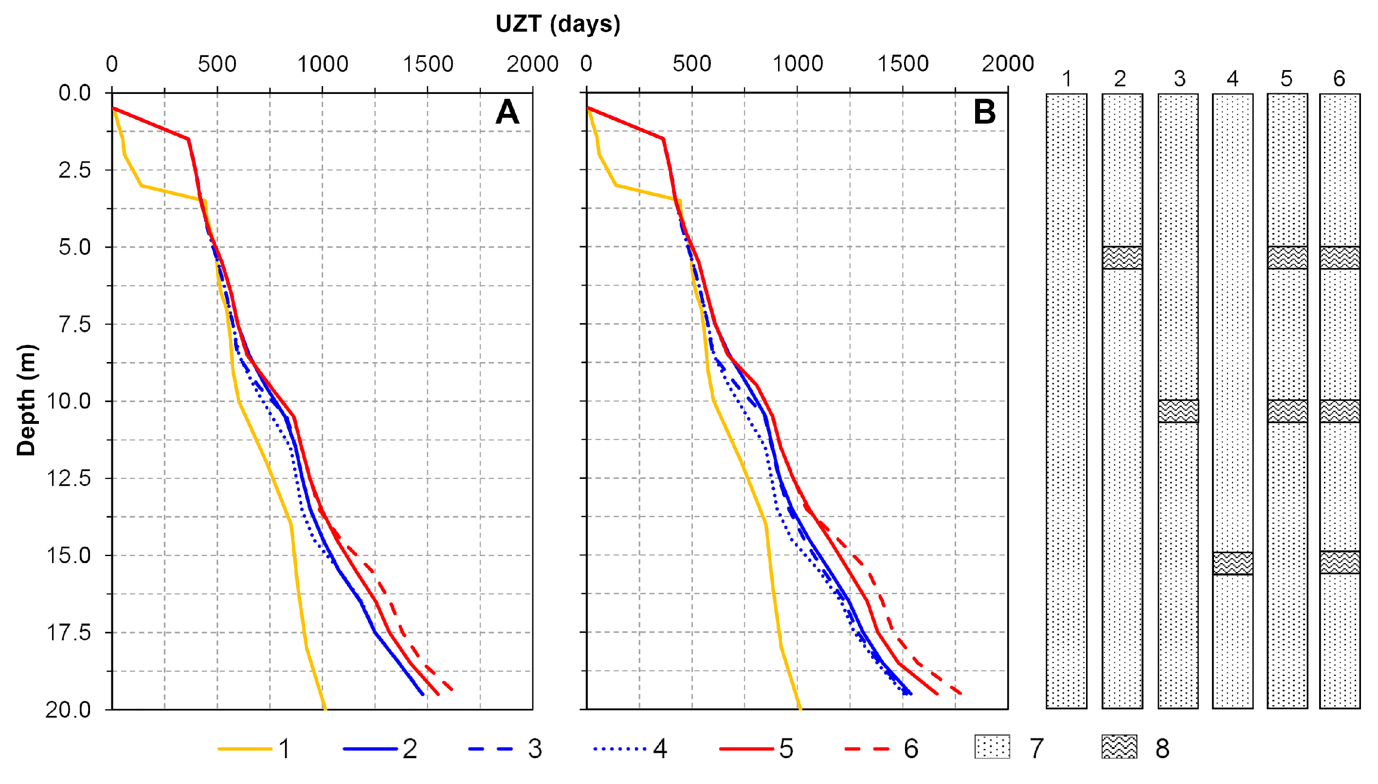
3.1. Hydro-Stratigraphic Models of the Unsaturated Zone

Considering the stratigraphic data of boreholes drilled in the study area, 18 representative conceptual hydro-stratigraphic models were identified, comprehending both homogeneous and heterogeneous soil columns of the unsaturated zone. In detail, six models were set as homogeneous soil columns with a single textural class. According to the observations and analyses of stratigraphic data of the alluvial-pyroclastic deposits forming the study area, the following USDA textural classes were recognized and considered for modeling: sand, loamy sand, sandy clay loam, sandy loam, loam, silty loam, and silt (Table 1). The other 12 models were set considering heterogeneous soil columns to simulate typically alternating settings of sandy loam deposits with one or more clay or silt horizon intercalations (Figure 4).
Initial hydrological conditions of the unsaturated zone were set according to the results of steady-state modeling of gravity drainage process starting from saturation (soil pressure head equal to zero; h = 0), which was carried out by the VS2DTI code. This modeling led to the simulation of water content and soil pressure head at the field capacity. In detail, the initial hydrological settings of the homogeneous hydro-stratigraphic models were arranged, depending on the soil textural classes (Table 1), with a soil pressure head varying from −1.0 m to −2.0 m at the upper boundary to 0.0 m at the water table. Unlike heterogeneous hydro-stratigraphic models, such a soil pressure head profile was articulated by specific values of soil pressure head assumed by the silt and clay horizons at the field capacity, varying from −1.0 m to −0.5 m, respectively. Values found for homogeneous hydro-stratigraphic models, constituted by loamy sand and sandy loam, were found to well-match those observed in preceding soil hydrological monitoring campaigns carried out on ash-fall pyroclastic deposits formed by the same textural classes in the peri-Vesuvian areas [70].
Concerning the boundary conditions, daily rainfall, evapotranspiration rates, and the time-varying parameters controlling water losses by evapotranspiration (Table 2) were applied to hydro-stratigraphic models at the upper boundary as climate forcings, starting from the beginning of September 2003 to the end of August 2013 (Figure 3).

3.2. UZT and Specific Aquifer Vulnerability to Nitrate Fertilizer Pollutant

Results of numerical modeling were analyzed to understand the hydrological response of the unsaturated zone of different 1D hydro-stratigraphic models and the associated differences on the propagation of the nitrate fertilizer pollutant through the unsaturated zone (Figure 4). Specifically, output data of modeling were initially analyzed to identify the UZT values of the pollutant for each observation point of the hydro-stratigraphic models considered.
Among the most relevant results is that UZT is not reliant on the initial concentration (C0). This observation led us to focus only on the effects on UZT of the depth to water table (D) and the equivalent saturated hydraulic conductivity along the vertical (Keq.z) (Figure 5, Figure 6 and Figure 7). Moreover, by the observation of the breakthrough curves of the pollutant, the daily Ci/C0 time series (Figure 5) showed peaks with a short delay (at least one day) from the spill input approximately down to the depth of 2.50 m with peaks characterized by a progressive delay, smoothing, and duration of the pollutant effects starting from 3.50 m of depth.
Results show how the seasonal hydrological variability of rainfall and evapotranspiration patterns strongly control the UZT of the pollutant in the very shallow parts, down to the depth of 0.5 m, which is affected by a strong seasonal fluctuations of water content determining a change in the unsaturated hydraulic conductivity and UZT (Figure 6). In detail, the data showed that pollutant needs up to 8–11 days to reach the depth of 0.5 m, leading to a very high groundwater vulnerability for this shallowest depth. This condition is enhanced, especially in the case of unsaturated zone formed by coarse soils such as loamy sand and sandy loam, for which short UZT values exist down to 3.0 and 2.0 m of depth. Although the lowest UZT values exist only for unsaturated zones formed by sandy soils, with 627 days needed for reaching the depth of 20.0 m, hydro-stratigraphic settings of the unsaturated zone formed by sandy loam, loam, loamy sand, and silt may also be considered representative of a high groundwater vulnerability with UZT values ranging between 365 days at 1.0 m to 503 days at 3.0 m. However, also in these conditions of higher groundwater vulnerability, the increase in the water table depth determines the rise of the UZT and the reduction of the groundwater vulnerability itself. Depending on the lower values of saturated hydraulic conductivity, finer soils forming the unsaturated zone induce greater UZT and the reduction of the groundwater vulnerability as, for example, in the case of a homogeneous hydro-stratigraphic model formed by sandy loam in comparison to one formed by silt. For these models, UZTs between 5.0 and 20.0 m of depth were observed varying respectively from 400 to 2100 days, in the case of sandy loam, and from 500 to 3088 days, in the case of silty soils.
The analysis of UZT values obtained considering the heterogeneous hydro-stratigraphic models, characterized by the combination of up to three stratigraphic soil horizons formed by different grain size classes, showed an increase in the values when more than one intercalation existed (Figure 7). Considering a hydro-stratigraphic setting formed by loamy sand with a single 1-m thick silt horizon located at three different depths (5.0, 10.0, and 15.0 m), UZT values at 20.0 m of depth were equal to 1475 days in all three cases. A similar condition exists for similar hydro-stratigraphic settings characterized by equivalent intercalations of a 1-m thick clay horizon, with the UZT equal to 1518 days at the depth of 20.0 m. Therefore, the UZT values were found to be not reliant on the depth of a single 1-m thick silt or clay horizon in all cases in which the estimation occurred at a depth greater than the silt or clay horizon. Instead, considering two and three 1-m thick silt or clay horizons, the UZT values observed at 20.0 m of depth were different, showing respective values from 1550 to 1639 days, considering intercalation of the silt horizons, and from 1662 to 1776 days in the case of the clay horizons.
Relationships between the UZT of the nitrate pollutant, depth to water table, and soil textural classes were analyzed and subdivided into five equal-interval classes to which respective groundwater vulnerability were associated varying from very low to very high (Table 3).
Based on the modeling results, the multiple correlation between UZT, water table depth (D), and equivalent saturated hydraulic conductivity along the vertical (Keq.z) of the unsaturated zone was analyzed. In detail, by analyzing the typical saturated hydraulic conductivity of each grain size class modeled, Ksat.eq. was estimated for each homogeneous and heterogeneous hydro-stratigraphic model. With these results, the following multiple correlation linking UZT with water table depth (D) and logarithm of Ksat.eq. (m/s) was found:
UZT   ( days )   =   1069.42   +   66.04   ·   D   ( m )     251.08   ·   Log   ( Ksat . eq   ( m / s ) )
This empirical law was found to be characterized by a high value of the multiple correlation coefficient (0.888), and a high statistical significance, with a value of probability of the null hypothesis by the Fisher’s test of 3 × 10−97. The multiple correlation describes an interpolating surface (Figure 8) showing a sloping that accounts for the increase in UZT values as the water table depth (D) increases and the equivalent hydraulic conductivity of the unsaturated zone (Ksat.eq) decreases.

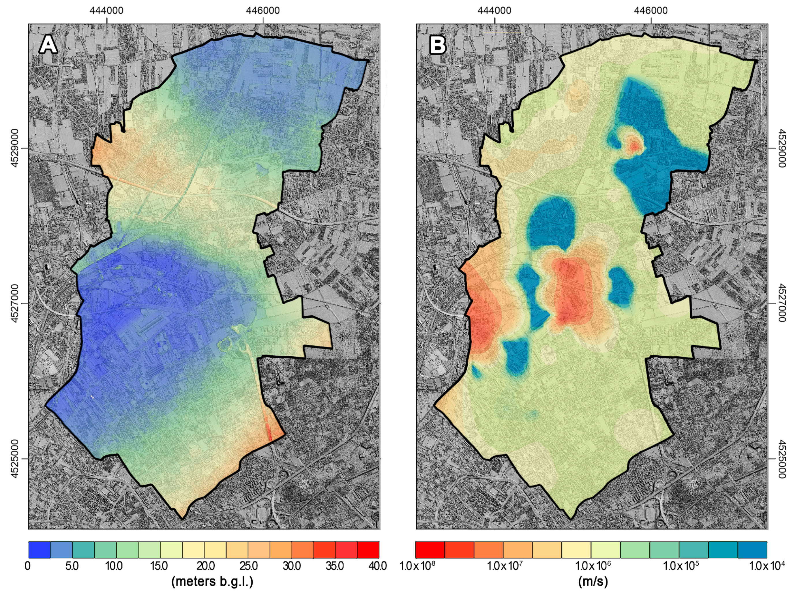
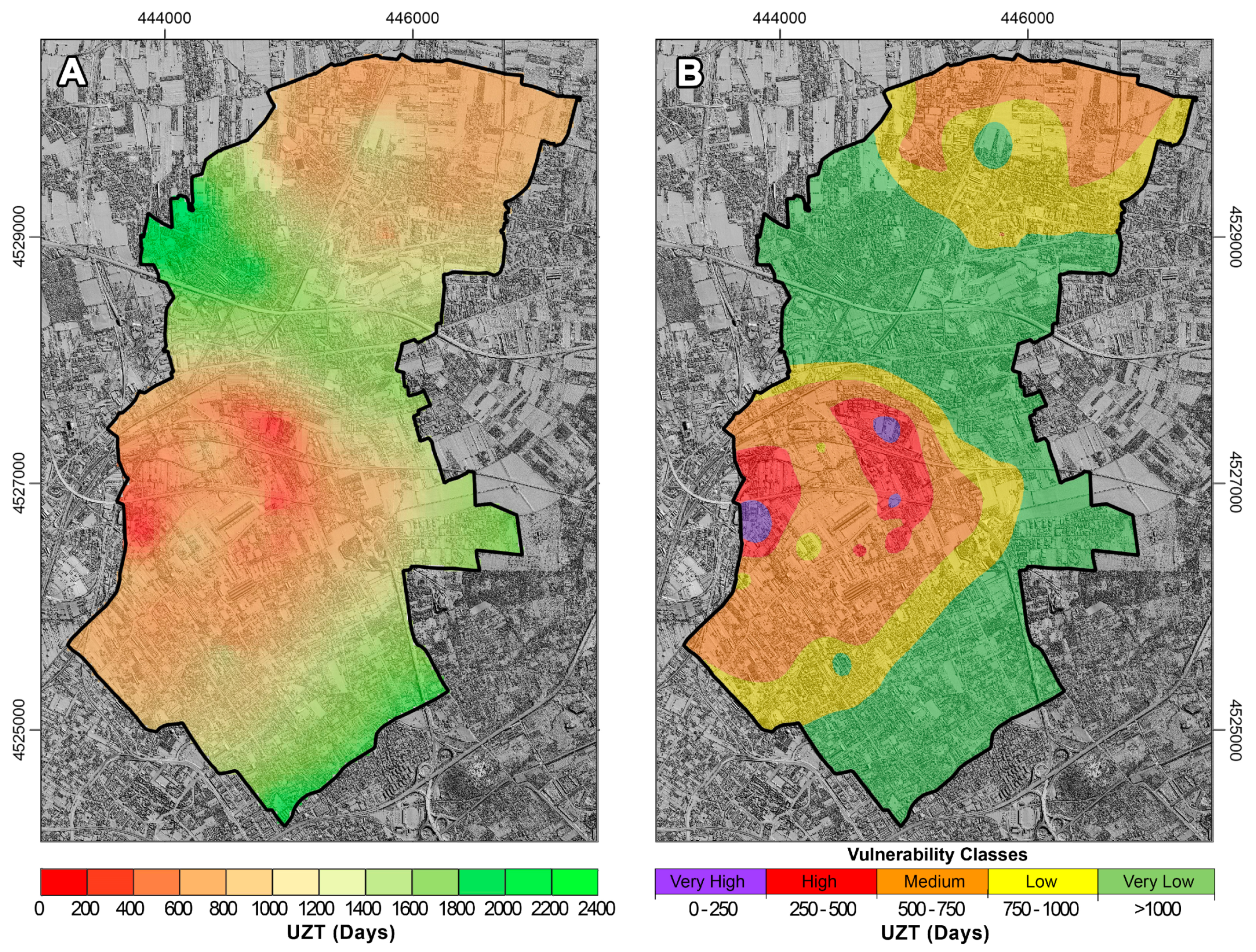
3.3. Distributed Assessment and Mapping of Groundwater Vulnerability

The empirical equation (Equation (2)) allowed us to assess and map specific aquifer vulnerability of the study area at a distributed scale. The equation was applied by a map calculator in QGIS by considering as dependent variables both the maps of water table depth (D) and logarithm of the equivalent hydraulic conductivity of the unsaturated zone (Log Ksat.eq.), at the resolution of 5 × 5 m respectively.
Specifically, the map of water table depth (D), reconstructed by the kriging spatial interpolation of piezometric surveys carried out in December 2013 over 108 wells [58,62] (Figure 9a), showed that the northern and central-western sectors of the study area were characterized by depth to water table mainly ranging between 1.0 and 5.0 m, even though very shallow conditions of water table depth (0.0–0.5 m) were also recognized. The remaining sectors of the study area were characterized by the deepest water table with values of depth exceeding 30.0 m.
The map of equivalent hydraulic conductivity (Ksat.eq.) of the unsaturated zone (Figure 9b) shows values that ranged mainly between 1.0 × 10⁻⁵ and 7.0 × 10⁻⁷ m/s, even if the central and northern sectors of the study area were characterized by lower values down to 1.0 × 10⁻⁸ m/s. However, very high values of Ksat.eq. existed in three well-defined sectors of the central sector of the Casalnuovo-Volla area, where such parameters reached the value of 1.0 × 10⁻⁴ m/s.
Starting from both maps of water table depth (D) and equivalent hydraulic conductivity of the unsaturated zone (Ksat.eq.), the empirical equation (Equation (2)) was applied to reconstruct a distributed map of UZT for the nitrate fertilizer pollutant (Figure 10a). Next, this map was classified according to the vulnerability classes identified (Table 3), thus a distributed groundwater specific vulnerability map to nitrate pollution was reconstructed for the study area (Figure 10b). In detail, the map shows how the northern, central, and southern sectors of the study area were characterized by low UZT values, mainly ranging between 400 and 900 days and corresponding to sectors with a shallower water table and higher Ksat.eq. of the unsaturated zone.
These sectors are characterized by specific aquifer vulnerability classes ranging from medium to high (Figure 10b). In particular, in the central sector, where the water table is very shallow or close to the ground surface, the UZT values reduced to few days and groundwater vulnerability comprised of the very high class. Instead, in the remaining sectors of the study area, the UZT values were higher, up to 2100 days, and intrinsic aquifer vulnerability ranged between the low and very low classes. Finally, as the central-northern sector was characterized by the deepest water table, UZT values reached values greater than 1200 days and groundwater vulnerability comprised of the very low class.

4. Discussion

In this study, representative hydro-stratigraphic models of the unsaturated zone of a shallow alluvial aquifer were used to assess specific vulnerability to nitrate fertilizer pollutants by modeling travel time through the unsaturated zone. This type of approach is widely adopted among those aimed at the quantitative assessment of groundwater vulnerability by physically based modeling [40,49,50,80,82]. Travel time modeling was carried out by the finite difference VS2DTI code [65] considering unsaturated/saturated soil properties, meteorological time series including daily evapotranspiration rates of 10 hydrological years (2003–2013), and a spill input of nitrate fertilizer, as typically applied by local farmers. The UZT values obtained by 1D modeling of pollutant transport were statistically correlated to water table depth (D) and equivalent saturated hydraulic conductivity (Ksat.eq.) of the unsaturated zone, obtaining an empirical model that was used to assess the UZT at a distributed scale for the study area.
Given the goal of the research, which was addressed to find a quantitative approach for the assessment of specific aquifer vulnerability to nitrate fertilizer pollutants, the latter was considered conservative with the purpose of taking into account the arrival time instead of concentrations of the pollutant at the water table [49,79]. In detail, the modeling results showed that polluted water propagates vertically through the unsaturated zone with yearly concentration waves that decrease their amplitude and increase their length with depth (Figure 5). This propagation is strongly affected by both rainfall distribution and soil hydrological conditions (soil pressure head regime). Close to the ground surface (down to 2.50 m of depth), breakthrough curves of the pollutant show high daily peaks of Ci/C0 rates following shortly rainfall events. Instead, starting from a depth of 3.50 m, down to the bottom boundary of the models, temporal distributions of the pollutant are characterized by breakthrough curves with smoothed and delayed peaks. This effect was more enhanced in sandy than loamy or silty soils due to the higher water retention capability of the latter.
Considering the results obtained for homogeneous hydro-stratigraphic settings, a very high groundwater vulnerability condition occurred for all grain size classes within the shallowest depth range of 0.5 m. For greater depth ranges of the water table, sand and loamy sand soil profiles of the unsaturated zone resulted in being the most vulnerable, showing a deepening of polluted percolation water faster than that estimated for the finer soils. For these grain size classes, the groundwater vulnerability results were high down to 2.0 and 3.0 m of the water table depth, respectively, while it was still medium down to the depth of 20.0 m in the case of sandy soils. Homogeneous hydro-stratigraphic models of the unsaturated zone formed by sandy loam, loam, and silty sand showed a similar hydrological response, thus similar vulnerability classes ranging from high, down to 3.0 m; medium, down 6.0 m; low, down 10.0 m; and very low, down to 20 m. Finally, the silty soil profile was less vulnerable as it showed a very low groundwater vulnerability, just below 7.0 m of depth (Table 3).
Results obtained by modeling heterogeneous hydro-stratigraphic models showed a similar hydrological behavior, although the effect of the intercalations of soil horizons with different grain sizes makes the propagation of the pollutant more complex. For hydro-stratigraphic models characterized by sandy loam, the number of intercalations of less-permeable soil horizons (silt and/or clay) controls the velocity of the pollutant transport more than their depth. In detail, the results of the UZT show that heterogeneous hydro-stratigraphic settings, with one soil horizon formed by silt or clay, but located at different depths, are characterized by the same groundwater vulnerability, if considering a water table at a depth greater than those of the less permeable soil horizons themselves. Furthermore, the increase in the number or thickness of less-permeable soil horizons also determines a decrease in UZT and groundwater vulnerability. Moreover, the results obtained allow us to recognize that UZT is not dependent on the initial concentration of the pollutant (C0), therefore it allowed us to disregard, according to the scope of this work, the attenuation of nitrate fertilizers in the root zone due to plant absorption as well as in the rest of the unsaturated zone [77,78,79]. Therefore, the UZT values, and the associated groundwater vulnerability, are strongly dependent on both depth and equivalent saturated hydraulic conductivity of the unsaturated zone (Ksat.eq.) above the water table level as has already been proven by other researchers [29,40]. Such recognition allowed us to estimate an empirical multiple correlation linking UZT to water table depth (D) and the equivalent saturated hydraulic conductivity (Ksat.eq.) of the unsaturated zone, which can be conceived as an innovative approach in the assessment of groundwater vulnerability for shallow alluvial aquifers to be used for the spatialization of modeling results.
The UZT values estimated by homogeneous and heterogeneous representative hydro-stratigraphic models indicate how the unsaturated hydraulic conductivity and its variability, depending on saturated hydraulic conductivity, unsaturated soil properties and soil pressure head, control the velocity of pollutant transport in the unsaturated zone. Analogously to other modeling approaches [40,82], the outcomes obtained reveal the strong seasonal control affecting the deepening of the infiltration front and the inherent transport of the pollutant through the unsaturated zone.
Even if similar studies have considered a quantitative approach to mapping aquifer vulnerability by combining flow and transport modeling, infiltration and transpiration rates with a solution of the advection-dispersion equation, the approach applied in this study may be considered innovative if compared to those obtained by the use of field data and tools of geographic information system (GIS) platforms [47] or in other cases coupled with the estimated travel time of pollutants through the vadose zone [5,10,35,37,49,50,80,82]. In fact, it can be conceived as advancing the others focused on the estimation of pollutant travel time through the unsaturated zone by a physically-based model based on the simplistic assumption of the lack of vertical gradients of soil pressure head and the applicability of the Darcy law in the unsaturated zone [50] or constant rainfall and evapotranspiration conditions [40]. In addition, the proposed approach can simplify the assessment of groundwater vulnerability in complex stratigraphic settings of alluvial aquifers, characterized by high 3D spatial variability [66], whose distributed modeling of UZT and pollutant concentrations at the water table would require the setting of complex process-based models (e.g., MT3D-MODFLOW [83]).

5. Conclusions

The proposed approach can be included among the methods applicable for the assessment of groundwater vulnerability at the site-specific scale, based on the numerical modeling of pollutant travel time through the unsaturated zone. It has been based on linking the results of UZT modeling for representative hydro-stratigraphic settings of the unsaturated zone to equivalent hydraulic conductivity of the unsaturated zone and water table depth by a bivariate empirical correlation that was used for the assessment of UZT across the whole study area.
In the framework of the Campania Trasparente Project, aimed at the assessment of the state of the quality of principal environmental matrices for the Campania region (southern Italy), the proposed approach was tested on the Casalnuovo-Volla sample area to assess the vulnerability of the shallow alluvial aquifer, which characterizes a large part of the internal and coastal plains of the region. The results of this study confirmed the potential strong impact of agricultural practice, based on the amendment of soils by nitrate fertilizers, on the hydro-chemical quality of the groundwater in the study area, which is largely characterized by shallow alluvial aquifers and intensive agricultural practice. The results obtained confirm the possibility of the existence of an anomalous concentration of nitrate in groundwater as has been reported in other studies [46,47,48] as well as that current concentrations of nitrate fertilizers in groundwater derive from the cumulative effects of fertilizing practice of the past and transport in the saturated zone. The recognition of the strong control of water table depth on UZT and groundwater vulnerability derives the important hint that groundwater vulnerability can vary in time depending on long-term piezometric fluctuations, which can occur due to natural or anthropogenic causes [58,62,64].
The proposed approach can be conceived as potentially applicable to produce specific vulnerability maps to nitrate pollution or other pollutant types for other areas of the Campanian Plain as well as other similar areas worldwide. For the latter, besides the local conditions of the water table depth and equivalent hydraulic conductivity, a specific numerical modeling of pollutant transport through the unsaturated zone should be carried out by considering the local meteorological patterns and timing of pollutant inputs. Finally, the proposed approach is considered as potentially applicable to similar hydrogeological frameworks of shallow alluvial aquifers where detailed stratigraphic as well as depth of water table data are available.

Author Contributions

Conceptualization, V.A. and P.D.V; data curation, F.F., S.C., D.C. and R.T.; formal analysis, P.D.V.; funding acquisition, V.A. and P.D.V.; investigation, F.F., V.A., S.C. and P.D.V.; methodology, F.F., V.A., D.C., R.T. and P.D.V.; resources, V.A.; software, F.F.; supervision, V.A. and P.D.V.; visualization, F.F., S.C., D.C. and R.T.; writing—original draft, F.F., S.C., D.C., R.T. and P.D.V.; writing—review & editing, V.A. and P.D.V. All authors have read and agreed to the published version of the manuscript.

Funding

This research was funded by Regione Campania (Decision of the Regional Government No. 497/2013 “Fondo per le Misure Anticicliche e la Salvaguardia dell’occupazione. Piano Terra dei Fuochi, Misura Campania Trasparente—Attività di monitoraggio integrato per la Regione Campania—Azione B4 “Mappatura del Territorio”)”.

Acknowledgments

We thank Antonio Limone (Istituto Zooprofilattico Sperimentale Del Mezzogiorno—IZSM) for the management of Campania Trasparente Project and Nunzio Romano (Interdepartmental Center for Environmental Research-CiRAM-University of Naples-Federico II) for the coordination of the section regarding the assessment of water quality.

Conflicts of Interest

The authors declare no conflict of interest.

References

  1. EU. Directive 2006/118/EC of the European Parliament and of the Council of 12 December 2006 on the protection of groundwater against pollution and deterioration. Off. J. Eur. Union 2006, 372, 19–31. [Google Scholar]
  2. EEA. European Union Emission Inventory Report 1990–2016 under the UNECE Convention on Long-Range Transboundary Air Pollution (LRTAP); EEA Report No 6/2018; EEA: Copenhagen, Denmark, 2018. [Google Scholar]
  3. Margat, J. Vulnérabilité des Nappes d’eau Souterraine à la Pollution; BRGM Publication: Orléans, France, 1968; p. 68. [Google Scholar]
  4. Foster, S.S.D. Fundamental Concepts in Aquifer Vulnerability, Pollution Risk and Protection Strategy. In Proceedings of the Vulnerability of Soil and Groundwater to Pollutants, The Hague, The Netherlands, 30 March 1987; pp. 69–86. [Google Scholar]
  5. Witkowski, A. Groundwater vulnerability and mapping. In Proceedings of the International Conference, Ustroń, Poland, 15–18 June 2004; p. 158. [Google Scholar]
  6. Civita, M. Le Carte Della Vulnerabilità Degli Acquiferi all’Inquinamento: Teoria e Pratica; Pitagora: Bologna, Italy, 1994; p. 344. [Google Scholar]
  7. Gogu, R.C.; Dassargues, A. Current trends and future challenges in groundwater vulnerability assessment using overlay and index methods. Environ. Geol. 2000, 39, 549–559. [Google Scholar] [CrossRef]
  8. National Research Council. Ground Water Vulnerability Assessment: Predicting Relative Contamination Potential Under Conditions of Uncertainty; The National Academies Press: Washington, DC, USA, 1993; p. 224. [Google Scholar]
  9. Vrba, J.; Zaporozec, A. Guidebook on Mapping Groundwater Vulnerability. IAH Int. Contrib. Hydrogeol. 1994, 16, 131. [Google Scholar]
  10. Zwahlen, F. Vulnerability and Risk Mapping for the Protection of Carbonate (Karst) Aquifers, Final Report COST Action 620; European Commission: Brussels, Belgium, 2004.
  11. Albinet, M.; Margat, J. Cartographie de la Vulnérabilité à la Pollution des Nappes d’eau Souterraine. Bull. BRGM 1970, 3, 13–22. [Google Scholar]
  12. Aller, L.; Bennet, T.; Lehr, J.H.; Petty, R.J.; Hackett, G. DRASTIC: A Standardized System for Evaluating Ground Water Pollution Potential Using Hydrogeological Settings; U.S. Environmental Protection Agency: Chicago, IL, USA, 1987; p. 266.
  13. Gogu, R.C.; Dassargues, A. Intrinsic vulnerability maps of a karstic aquifer as obtained by five different assessment techniques: Comparison and comments. In Proceedings of the 7th Conference on Limestone Hydrology and Fissured Media, Besançon, France, 20–22 September 2001. [Google Scholar]
  14. Goldscheider, N. Karst groundwater vulnerability mapping: Application of a new method in the Swabian Alb, Germany. Hydrogeol. J. 2005, 13, 555–564. [Google Scholar] [CrossRef]
  15. Andreo, B.; Goldscheider, N.; Vadillo, J.; Vias, J.; Neukum, C.; Sinreich, M. Karst groundwater protection: First application of a Pan-European approach to vulnerability, hazard and risk mapping in the Sierra de Libar (Southern Spain). Sci. Total Environ. 2006, 357, 54–73. [Google Scholar] [CrossRef]
  16. Van Stempvoort, D.; Evert, L.; Wassenaar, L. Aquifer vulnerability index: A GIS compatible method for groundwater vulnerability mapping. Can. Water Resour. J. 1993, 18, 25–37. [Google Scholar] [CrossRef] [Green Version]
  17. Civita, M.; De Maio, M. Valutazione e cartografia automatica della vulnerabilità degli acquiferi all’inquinamento con il sistema parametrico SINTACS R5 (SINTACS R5, a parametric system for the assessment and automatic mapping of groundwater vulnerability to contamination); Pitagora: Bologna, Italy, 2000; p. 248. [Google Scholar]
  18. Celico, F. Vulnerabilità all’inquinamento degli acquiferi e delle risorse idriche sotterranea in realtà idrogeologiche complesse: I metodi DAC e VIR. Quaderni di Geologia Applicata 1996, 3, 93–116. [Google Scholar]
  19. Civita, M.; De Regibus, C. Sperimentazione di alcune metodologie per la valutazione della vulnerabilità degli acquiferi, Quaderni di Geologia Applicata. Pitagora Editrice 1995, 3, 63–71. [Google Scholar]
  20. Hölting, B.; Haertle, T.; Hohberger, K.H.; Nachtigall, K.H.; Villinger, E.; Weinzierl, W. Konzept zur Ermittlung der Schutzfunktion der Grundwasserüberdeckung. Geologisches Jahrbuch der BGR 1995, 6, 5–24. [Google Scholar]
  21. Goldscheider, N.; Klute, M.; Sturm, S.; Hötzl, H. The PI method–a GIS-based approach to mapping groundwater vulnerability with special consideration of karst aquifers. Zeitschrift für Angewandte Geologie 2000, 463, 157–166. [Google Scholar]
  22. Doerfliger, N.; Jeannin, P.Y.; Zwahlen, F. Water vulnerability assessment in karst environments: A new method of defining protection areas using a multiattribute approach and GIS tools (EPIK method). Environ. Geol. 1999, 39, 165–176. [Google Scholar] [CrossRef] [Green Version]
  23. Focazio, M.J.; Reilly, T.E.; Rupert, M.G.; Helsel, D.R. Assessing Ground-Water Vulnerability to Contamination: Providing Scientifically Defensible Information for Decision Makers; US Department of Interior and US Geological Survey: Reston, VA, USA, 2002.
  24. Rupert, M.G. Calibration of the DRASTIC Ground Water Vulnerability Mapping Method. Ground Water 2001, 39, 625–630. [Google Scholar] [CrossRef] [PubMed]
  25. McLay, C.D.A.; Dragten, R.; Sparling, G.; Selvarajah, N. Predicting groundwater nitrate concentrations in a region of mixed agricultural land use: A comparison of three approaches. Environ. Pollut. 2001, 115, 191–204. [Google Scholar] [CrossRef]
  26. Panagopoulos, G.P.; Antonakos, A.K.; Lambrakis, N.J. Optimization of the DRASTIC method for groundwater vulnerability assessment via the use of simple statistical methods and GIS. Hydrogeol. J. 2006, 14, 894–911. [Google Scholar] [CrossRef]
  27. Antonakos, A.K.; Lambrakis, N.J. Development and testing of three hybrid methods for the assessment of aquifer vulnerability to nitrates, based on the drastic model, an example from NE Korinthia, Greece. J. Hydrol. 2007, 333, 288–304. [Google Scholar] [CrossRef]
  28. Huan, H.; Wang, J.; Teng, Y. Assessment and validation of groundwater vulnerability to nitrate based on a modified DRASTIC model: A case study in Jilin City of northeast China. Sci. Total Environ. 2012, 440, 14–23. [Google Scholar] [CrossRef]
  29. Kazakis, N.; Voudouris, K.S. Groundwater vulnerability and pollution risk assessment of porous aquifers to nitrate: Modifying the DRASTIC method using quantitative parameters. J. Hydrol. 2015, 525, 13–25. [Google Scholar] [CrossRef]
  30. Brindha, K.; Elango, L. Cross comparison of five popular groundwater pollution vulnerability index approaches. J. Hydrol. 2015, 524, 597–613. [Google Scholar] [CrossRef]
  31. Frind, E.O.; Molson, J.W.; Rudolph, D.L. Well vulnerability: A quantitative approach for source water protection. Ground Water 2006, 44, 732–742. [Google Scholar] [CrossRef]
  32. Gogu, R.C.; Hallet, V.; Dassargues, A. Comparison of aquifer vulnerability assessment techniques. Application to the Neblon River basin (Belgium). Environ. Geol. 2003, 44, 881–892. [Google Scholar] [CrossRef]
  33. Merchant, J.W. GIS-based groundwater pollution hazard assessment: A critical review of the DRASTIC model. Photogramm. Eng. Remote Sens. 1994, 60, 1117–1127. [Google Scholar]
  34. Jeannin, P.Y.; Grainaton, F.; Zwahlen, F.; Perrochet, P. VULK: A tool for intrinsic vulnerability assessment and validation. In Proceedings of the 7th Conference on Limestone, Hydrology and Fissured Media, Besançon, France, 20–22 September 2001. [Google Scholar]
  35. Connell, L.D.; Van den Daele, G. A quantitative approach to aquifer vulnerability mapping. J. Hydrol. 2003, 276, 71–88. [Google Scholar] [CrossRef]
  36. Witkowski, A.J.; Kowalczyk, A. A simplified method of regional groundwater vulnerability assessment. In Proceedings of the Groundwater Vulnerability and Mapping International Conference, Ustroń, Poland, 15–18 June 2004. [Google Scholar]
  37. Voigt, H.J.; Heinkele, T.; Wolter, R. Characterization of groundwater vulnerability in Germany. In Proceedings of the Groundwater Vulnerability Assessment and Mapping International Conference, Ustroń, Poland, 15–18 June 2004. [Google Scholar]
  38. Brouyère, S.; Jeannin, P.Y.; Dassargues, A.; Goldscheider, N.; Popescu, I.C.; Sauter, M.; Vadillo, I.; Zwahlen, F. Evaluation and validation of vulnerability concepts using a physically based approach. In Proceedings of the 7th Conference on Limestone Hydrology and Fissured Media, Mémoire no. 13, Sciences et Techniques de l’Environnement, Université de Franche-Comté, Besançon, France, 20–22 September 2001. [Google Scholar]
  39. Jarvis, N. The MACRO Model (Version 4.3) Technical Description; Department of Soil Sciences, Swedish University of Agricultural Sciences (SLU): Uppsala, Sweden, 2002; p. 37. [Google Scholar]
  40. Neukum, C.; Azzam, R. Quantitative assessment of intrinsic groundwater vulnerability to contamination using numerical simulations. Sci. Total Environ. 2009, 408, 245–254. [Google Scholar] [CrossRef] [PubMed]
  41. Stewart, I.T.; Loague, K. Assessing ground water vulnerability with the type transfer function model in the Joaquin Valley, California. J. Environ. Qual. 2004, 33, 1487–1498. [Google Scholar] [CrossRef]
  42. Knisel, W.G. GLEAMS, Groundwater Loading Effects of Agricultural Management Systems; Version 2.10; Biological and Agricultural Engineering Department, Coastal Plain Experiment Station, University of Georgia: Tifton, GA, USA, 1993; p. 260. [Google Scholar]
  43. Knisel, W.G.; Davis, F.M. GLEAMS: Groundwater Loading Effects from Agricultural Management Systems, version 3.0; Biological and Agricultural Engineering Department, Coastal Plain Experiment Station, University of Georgia: Tifton, GA, USA, 2000; Publication No. SEWRL-WGK/FMD-050199. [Google Scholar]
  44. Šimunek, J.; Šejna, M.; Saito, H.; Sakai, M.; Van Genuchten, M.T.H. The HYDRUS-1D Software Package for Simulating the Movement of Water, Heat, and Multiple Solutes in Variably Saturated Media, version 4.08; University of California: Riverside, CA, USA, 2009. [Google Scholar]
  45. Aschonitis, V.G.; Mastrocicco, M.; Colombani, N.; Salemi, E.; Kazakis, N.; Voudouris, K.; Castaldelli, G. Assessment of the intrinsic vulnerability of agricultural land to water and nitrogen losses via deterministic approach and regression analysis. Water Air Soil Pollut. 2012, 223, 1605–1614. [Google Scholar] [CrossRef]
  46. Celico, P.; Esposito, L.; Guadagno, F.M. Sulla qualità delle acque sotterranee nell’acquifero del settore orientale della Piana Campana. Geologia Tecnica e Ambientale 1997, 4, 17–27. [Google Scholar]
  47. Corniello, A.; Ducci, D.; Ruggieri, G. Areal Identification of Groundwater Nitrate Contamination Sources in Periurban Areas. J. Soils Sediments 2007, 7, 159–166. [Google Scholar] [CrossRef]
  48. Ducci, D.; Della Morte, R.; Mottola, A.; Onorati, G.; Pugliano, G. Nitrate trends in groundwater of the Campania region (southern Italy). Environ. Sci. Pollut. Res. 2019, 26, 2120–2131. [Google Scholar] [CrossRef]
  49. Wang, L.; Stuart, M.E.; Bloomfield, J.P.; Butcher, A.S.; Gooddy, D.C.; McKenzie, A.A.; Lewis, M.A.; Williams, A.T. Prediction of the arrival of peak nitrate concentrations at the water table at the regional scale in Great Britain. Hydrol. Process. 2012, 26, 226–239. [Google Scholar] [CrossRef] [Green Version]
  50. Fetisova, N.F.; Fetisov, F.F.; De Maio, M.; Zektser, I.S. Groundwater vulnerability assessment based on calculation of chloride travel time through the unsaturated zone on the area of the Upper Kama potassium salt deposit. Environ. Earth Sci. 2016, 75, 681. [Google Scholar] [CrossRef]
  51. Rolandi, G.; Petrosino, P.; McGeehin, J. The interplinian activity at Somma-Vesuvius in the last 3500 years. J. Volcanol. Geotherm. Res. 1998, 82, 19–52. [Google Scholar] [CrossRef]
  52. Rolandi, G.; Bellucci, F.; Heizler, M.T.; Belkin, H.E.; De Vivo, B. Tectonic controls on the genesis of ignimbrites from the Campanian volcanic zone, southern Italy. Mineral. Petrol. 2003, 79, 3–31. [Google Scholar] [CrossRef]
  53. Bellucci, F. Nuove conoscenze stratigrafiche sui depositi effusivi ed esplosivi nel sottosuolo dell’area del Somma-Vesuvio. Boll. Della Soc. Geol. Ital. 1998, 117, 385–405. [Google Scholar]
  54. Ruberti, D.; Vigliotti, M.; Marzaioli, R.; Pacifico, A.; Ermice, A. Stratigraphic architecture and anthropic impacts on subsoil to assess the intrinsic potential vulnerability of groundwater: The northeastern Campania Plain case study, southern Italy. Environ. Earth Sci. 2014, 71, 319–339. [Google Scholar] [CrossRef]
  55. De Vita, P.; Allocca, V.; Celico, F.; Fabbrocino, S.; Mattia, C.; Monacelli, G.; Musilli, I.; Piscopo, V.; Scalise, A.R.; Summa, G.; et al. Hydrogeology of continental southern Italy. J. Maps 2018, 14, 230–241. [Google Scholar]
  56. Allocca, V.; Celico, P. Scenari idrodinamici nella piana ad Oriente di Napoli (Italia) nell’ultimo secolo: Cause e problematiche idrogeologiche connesse. G. Geol. Appl. 2008, 9, 175–198. [Google Scholar]
  57. Esposito, L.; Piscopo, V. Groundwater flow evolution in the Campanian-Plain. In Proceedings of the 27th Congress of the International Association of Hydrogeologist, Notthingham, UK, 21–27 September 1997. [Google Scholar]
  58. Coda, S.; Tessitore, S.; Di Martire, D.; Calcaterra, D.; De Vita, P.; Allocca, V. Coupled ground uplift and groundwater rebound in the metropolitan city of Naples (southern Italy). J. Hydrol. 2019, 569, 470–482. [Google Scholar] [CrossRef]
  59. De Vivo, B.; Rolandi, G.; Gans, P.B.; Calvert, A.; Bohrson, W.A.; Spera, F.J.; Belkin, A.E. New constraints on the pyroclastic eruption history of the Campanian volcanic plain (Italy). Mineral. Petrol. 2001, 73, 47–65. [Google Scholar] [CrossRef]
  60. Celico, P.; Esposito, L.; De Gennaro, M.; Mastrangelo, E. La falda ad Oriente della città di Napoli: Idrodinamica e qualità delle acque. Geol. Romana 1994, 30, 653–660. [Google Scholar]
  61. Esposito, L. Nuove conoscenze sulle caratteristiche idrogeochimiche della falda ad Oriente della città di Napoli (Campania). Quad. Di Geol. Appl. 1998, 5, 5–14. [Google Scholar]
  62. Coda, S.; Tessitore, S.; Di Martire, D.; De Vita, P.; Allocca, V. Enviromental effects of the groundwater rebound in the easter plain of Naples (Italy). Rendiconti Online Società Geologica Italiana 2019, 48, 35–40. [Google Scholar] [CrossRef]
  63. Allocca, V.; Coda, S.; De Vita, P.; Iorio, A.; Viola, R. Rising groundwater levels and impacts in urban and semirural areas around Naples (southern Italy). Rendiconti Online Della Società Geologica Italiana 2016, 41, 14–17. [Google Scholar] [CrossRef]
  64. Coda, S.; Confuorto, P.; De Vita, P.; Di Martire, D.; Allocca, V. Uplift Evidences Related to the Recession of Groundwater Abstraction in a Pyroclastic-Alluvial Aquifer of Southern Italy. Geosciences 2019, 9, 215. [Google Scholar] [CrossRef] [Green Version]
  65. Hsieh, P.A.; Wingle, W.; Healy, R.W. VS2DI-a graphical software package for simulating fluid flow and solute or energy transport in variably saturated porous media. U.S. Geol. Surv. Water Resour. Investig. Rep. 2000, 99–4130, 16. [Google Scholar]
  66. Ducci, D.; Sellerino, M. Vulnerability mapping of groundwater contamination based on 3D lithostratigraphical models of porous aquifers. Sci. Total Environ. 2013, 447, 315–322. [Google Scholar] [CrossRef] [PubMed]
  67. van Genuchten, M.T. A closed-form equation for predicting the hydraulic conductivity of unsaturated soils. Soil Sci. Soc. Am. J. 1980, 44, 892–898. [Google Scholar] [CrossRef] [Green Version]
  68. Lappala, E.G.; Healy, R.W.; Weeks, E.P. Documentation of computer program VS2D to solve the equations of fluid flow in variably saturated porous media. U.S. Geol. Surv. Water Resour. Investig. Rep. 1987, 83–4099, 184. [Google Scholar]
  69. Carsel, R.F.; Parrish, R.S. Developing joint probability distributions of soil water retention characteristics. Water Resour. Res. 1988, 24, 755–769. [Google Scholar] [CrossRef] [Green Version]
  70. Fusco, F.; Allocca, V.; De Vita, P. Hydro-geomorphological modelling of ash-fall pyroclastic soils for debris flow initiation and groundwater recharge in Campania (southern Italy). Catena 2017, 158, 235–249. [Google Scholar] [CrossRef]
  71. Hargreaves, G.L.; Samani, Z.A. Reference crop evapotranspiration from temperature. Adv. Water Resour. 1985, 111, 113–124. [Google Scholar] [CrossRef]
  72. Allen, D.J.; Brewerton, L.J.; Coleby, L.M.; Gibbs, B.R.; Lewis, M.A.; MacDonald, A.M.; Wagstaff, S.J.; Williams, A.T. The Physical Properties of Major Aquifers in England and Wales; Technical Report WD/97/34; British Geological Survey: Nottingham, UK, 1997; p. 312. [Google Scholar]
  73. Batu, V. Applied Flow and Solute Transport Modelling in Aquifers; Taylor and Francis Group: Abingdon, UK, 2005; ISBN 0-8493-3574-4. [Google Scholar]
  74. Schulze-Makuch, D. Longitudinal Dispersivity Data and Implications for Scaling Behavior. Ground Water 2005, 43, 443–456. [Google Scholar] [CrossRef] [PubMed]
  75. Clement, J.C.; Pinay, G.; Marmonier, P. Seasonal dynamics of denitrification along topohydrosequences in three different riparian wetlands. J. Environ. Qual. 2002, 31, 1025–1037. [Google Scholar] [CrossRef] [PubMed]
  76. Jahangir, M.M.R.; Khalil, M.I.; Johnston, P.; Cardenas, L.M.; Hatch, D.J.; Butler, M.; Barrett, M.; O’Flaherty, V.; Richards, K.G. Denitrification potential in subsoils: A mechanism to reduce nitrate leaching to groundwater. Agric. Ecosyst. Environ. 2012, 147, 13–23. [Google Scholar] [CrossRef] [Green Version]
  77. Kinninburg, D.G.; Gale, I.N.; Goody, D.C.; Darling, W.G.; Marks, R.J.; Gibbs, B.R.; Coleby, L.M.; Bird, M.J.; West, J.M. Denitrification in the unsaturated zones of the British Chalk and Sherwood Sandstone aquifers; Technical Report WD/99/2; British Geological Survey: Nottingham, UK, 1999. [Google Scholar]
  78. Rivett, M.O.; Smith, J.W.N.; Buss, S.R.; Morgan, P. Nitrate occurrence and attenuation in the major aquifers of England and Wales. Q. J. Eng. Geol. Hydrogeol. 2007, 40, 335–352. [Google Scholar] [CrossRef]
  79. Ascott, M.J.; Wang, L.; Stuart, M.E.; Ward, R.S.; Hart, A. Quantification of nitrate storage in the vadose (unsaturated) zone: A missing component of terrestrial N budgets. Hydrol. Process. 2016, 30, 1903–1915. [Google Scholar] [CrossRef] [Green Version]
  80. Yu, C.; Yao, Y.; Hayes, G.; Zhang, B.; Zheng, C. Quantitative assessment of groundwater vulnerability using index system and transport simulation, Huangshuihe catchment, China. Sci. Total Environ. 2010, 408, 6108–6116. [Google Scholar] [CrossRef]
  81. Freeze, R.A.; Cherry, J.A. Groundwater; Prentice-Hall: Englewood Cliffs, NJ, USA, 1979; p. 604. [Google Scholar]
  82. Nolan, B.T.; Green, C.T.; Juckem, P.F.; Liao, L.; Reddy, J.E. Metamodeling and mapping of nitrate flux in the unsaturated zone and groundwater, Wisconsin, USA. J. Hydrol. 2018, 559, 428–441. [Google Scholar] [CrossRef]
  83. Almasri, M.N.; Kaluarachchi, J.J. Modeling nitrate contamination of groundwater in agricultural watersheds. J. Hydrol. 2007, 343, 211–229. [Google Scholar] [CrossRef]
Figure 1. (a) Hydrogeological map of the eastern plain of Naples [55 modified] and (b) study area. Legend: (1) epiclastic continental complex; (2) travertines complex; (3) ash fall pyroclastic complex; (4) ash flow pyroclastic complex; (5) lava complex; (6) carbonate complex; (7) normal fault; (8) piezometric contour line (m a.s.l.); (9) groundwater flow direction; (10) groundwater divide; (11) wells and piezometers considered for measures of piezometric levels; (12) borehole; (13) sector with buried CI; (14) trace of hydrogeological cross-section (Figure 2); (15) rivers connected with groundwater circulation; (16) rivers with negligible or null interactions with groundwater circulation due to ephemeral regime or waterproofing of riverbed by cementing; (17) Lufrano’s well field of (a), Acerra (b) and Ponticelli (c); and (18) study area.
Water 12 00269 g001
Figure 2. Hydrogeological cross-sections of the aquifer system. Legend: (1) silty sands; (2) pumiceous lapilli horizons; (3) sands; (4) marshy clay-sand and clay-silt levels; (5) incoherent or semi-lithoid lavas; (6) lithoid (a) and incoherent (b) CI tuff; (7) lapilli and coarse sands deposits; (8) phreatic (a) and semi-confined (b) piezometric level; and (9) borehole.
Water 12 00269 g002
Figure 3. Daily rainfall and evapotranspiration rates (from the beginning of September 2003 to the end of August 2013) applied as climate boundary conditions to VS2DTI modeling.
Water 12 00269 g003
Figure 4. Example of numerical modeling of pollutant propagation throughout the unsaturated zone of a heterogeneous hydro-stratigraphic model, performed by VS2DTI code: (A) heterogeneous hydro-stratigraphic model with three silt intercalated layers; (B) results of pollutant propagation at the end of the 10-year simulation period. Keys to symbols: (1) loamy sand soil; (2) silt intercalated layer; (3) Neapolitan Yellow Tuff (NYT), external to the modeled domain; (4) flux into the domain (infiltration); (5) possible seepage face; (6) outflow from the domain (evapotranspiration); (7) no-flux boundary; and (8) observation point.
Water 12 00269 g004
Figure 5. Example of a modeled breakthrough curve of nitrate pollutant, expressed as the ratio Ci/C0, obtained for the homogeneous loamy sand soil hydro-stratigraphic model and by setting one-day spill inputs of nitrate fertilizer pollutant with different concentrations: (A) 1.0 mg/L; (B) 3.0 mg/L.
Water 12 00269 g005
Figure 6. Variation of the Unsaturated Zone travel Time (UZT) with depth and textural classes obtained from homogeneous hydro-stratigraphic models.
Water 12 00269 g006
Figure 7. Variation of UZT and depth obtained for heterogeneous hydro-stratigraphic models characterized by a homogeneous (1) soil column of loamy sand, with a single (2, 3, 4) double (5) or triple (6) 1-m thick intercalation of silt (A) or clay (B) located at different depths. Other keys to symbols: (7) loamy sand; (8) silt or clay.
Water 12 00269 g007
Figure 8. Bivariate empirical correlation between UZT, water table depth (D), and the equivalent hydraulic conductivity of the unsaturated zone values (Ksat.eq) reconstructed by the results of homogenous and heterogeneous hydro-stratigraphic models.
Water 12 00269 g008
Figure 9. (A) Water table depth map; (B) equivalent saturated hydraulic conductivity (Ksat.eq.) of the unsaturated zone related to the Casalnuovo-Volla alluvial aquifer.
Water 12 00269 g009
Figure 10. (A) UZT map of nitrate fertilizer pollutant through the unsaturated zone of the Casalnuovo-Volla alluvial aquifer; (B) groundwater vulnerability map.
Water 12 00269 g010
Table 1. Values of hydraulic properties used for numerical modeling derived by the VS2DTI catalog for generic soil textural classes based on the classification of United States Department of Agriculture (USDA) [68,69]. Key to symbols: Ksat = saturated hydraulic conductivity; p = porosity; RMC = residual soil moisture content; α and n = van Genuchten’s fitting parameters.
Soil TypeKsat (m/s)p (-)RMC (-)α (cm−1)n (-)
Sand4.63 × 10−30.370.0204.313.10
Loamy Sand2.43 × 10−50.410.05712.402.28
Sandy Clay Loam8.10 × 10−50.500.0150.854.80
Sandy Loam1.23 × 10−50.410.0657.501.89
Loam2.89 × 10−60.430.0783.601.56
Silty Loam2.60 × 10−60.450.0672.001.41
Silt6.94 × 10−70.460.0341.601.37
Table 2. (A) Values of the time-varying parameters controlling water losses by evapotranspiration used for numerical modeling: RD = rooting depth; RAT = root activity at top; RAB = root activity at base; RPH = root pressure head. (B) Hydrodynamic parameters for nitrates: CMD = coefficient of molecular diffusion from [73]; DC = constant for first-order decay; LD and TD = longitudinal and transverse dispersivity, respectively.
ARD (m)RAT (cm−2)RAB (cm−2)RPH (m)
0.301.001.00−100
BCMD (m2/s)DC (-)LD (-)TD (-)
1.77 × 10−90.00.10.1
Table 3. UZT (days) estimated for different grain size classes and different depths of water table, down to 20 m. Lower table: groundwater vulnerability classes based on equal interval classification of UZT values.
UZT (days)
Depth (m)0.589911888
1.082937394366365369
2.038359130433417401427
3.0386139460495470434503
4.0398450500558542492576
5.0411491553587594550728
6.0415505567731713587874
7.04235446578538616821001
8.04435638108889198141214
9.045357584195710318691358
10.0472603869110711999151520
12.049373510031338142011512010
14.052685112241537169413472263
16.055388313511933203514902742
18.056192416332081217718252851
20.0627101518852215235920243088
SandLoamy SandSandLoamSandy LoamLoamSilty SandSilt
Grain Size Classes
Vulnerability Classes
0 ÷ 250251 ÷ 500501 ÷ 750751 ÷ 1000>1000
Very HighHighMediumLowVery Low

