Estimating Soil Organic Carbon in Agricultural Gypsiferous Soils by Diffuse Reflectance Spectroscopy
by
 ,
,
Maria Jose Marques
1,* ,
,
Ana María Álvarez
1, 
Pilar Carral
1,
Iris Esparza
2,
Blanca Sastre
2 and
Ramón Bienes
2 1
Geology and Geochemistry Department, Faculty of Sciences, Autonomous University of Madrid, Calle Francisco Tomás y Valiente, 7, 28049 Madrid, Spain
2
Departamento de Investigación Aplicada y Extensión Agraria, Instituto Madrileño de Investigación y Desarrollo Rural, Agrario y Alimentario (IMIDRA), Finca El Encín. Autovía A-2 km 38.2, 28800 Alcalá, Spain
*
Author to whom correspondence should be addressed.
Water 2020, 12(1), 261; https://doi.org/10.3390/w12010261
Submission received: 18 December 2019
/
Revised: 9 January 2020
/
Accepted: 13 January 2020
/
Published: 16 January 2020
(This article belongs to the Special Issue Soil Erosion, Soil Desertification and Soil Conservation in Agri-Environment Systems)
Abstract
:Contents of soil organic carbon (SOC), gypsum, CaCO3, and quartz, among others, were analyzed and related to reflectance features in visible and near-infrared (VIS/NIR) range, using partial least square regression (PLSR) in ParLes software. Soil samples come from a sloping olive grove managed by frequent tillage in a gypsiferous area of Central Spain. Samples were collected in three different layers, at 0–10, 10–20 and 20–30 cm depth (IPCC guidelines for Greenhouse Gas Inventories Programme in 2006). Analyses were performed by C Loss-On-Ignition, X-ray diffraction and water content by the Richards plates method. Significant differences for SOC, gypsum, and CaCO3 were found between layers; similarly, soil reflectance for 30 cm depth layers was higher. The resulting PLSR models (60 samples for calibration and 30 independent samples for validation) yielded good predictions for SOC (R2 = 0.74), moderate prediction ability for gypsum and were not accurate for the rest of rest of soil components. Importantly, SOC content was related to water available capacity. Soils with high reflectance features held c.a. 40% less water than soils with less reflectance. Therefore, higher reflectance can be related to degradation in gypsiferous soil. The starting point of soil degradation and further evolution could be established and mapped through remote sensing techniques for policy decision making.
1. Introduction
Soil formation in dry environments has been shaped by limited precipitation and high evapotranspiration, with an incomplete lixiviation of lime, gypsum or other salts in soils layers. When these arid or semi-arid soils are farmed, erosion processes lead to the loss of topsoil which is usually enriched in soil organic carbon (SOC) and nutrients. Consequently, lime- and/or gypsum-enriched subsoil layers emerge, and the reflectance properties of soil change.
Since the 1990s, soil spectral signatures—that is, the reflectance or absorption of soils at the different wavelengths of the electromagnetic spectrum—have been confirmed as a fast, reliable and cheap method to determine the physicochemical characteristics of those soils ([1,2,3,4,5]; this is the base of the chemometric approach, with multiple uses in environmental studies.
The analysis of visible and near-infrared (VIS/NIR) spectroscopy refers to the reflectance of materials in the 350–2500 nm region of the spectrum. Considering soils, their spectral signatures are linear combinations of soil components depending on their nature and abundance [6]. Thus, small changes in soil composition can be detected through their changes in spectral signatures.
There is a need to carry out specific analysis of spectral signatures at the local level due to the great variety of soil types in the world, which are determined by different proportions of soil components. For example, spectrometry can be used to determine soil iron content [7,8], or soil organic carbon [9,10,11] or texture [12]. National and international spectral libraries are collecting massive data of geological and edaphological information [13], being a valuable legacy and a useful tool for mapping purposes [14]. From the chemometric point of view, there is no need for large libraries to obtain reliable results at the local level [15]. Spectral libraries must be effectively used to determine or predict physical–chemical characteristics [2,16,17,18,19], but also to infer soil properties and their evolution over time and space [20,21,22]. This is especially important in the current context of a need for soil degradation control. Spectrometry alone or combined with remote sensing has been recognized as efficient methods to evaluate land degradation [23,24,25,26] or to manifest soil processes [27]. Different examples of use are the effects of wildfires [15,28], heavy metal pollution [29], or salt accumulation [30,31]. The assessment of soil erosion by these techniques has been addressed widely [32,33,34,35]. Such approaches are crucial in decision making for environmental protection.
One of the most promising lines of research for the assessment of soil characteristics from spectrometry and remote sensing is related to soil organic matter content. This approach was soon addressed by researchers, in the beginning, to determine the optimum wavelengths for predicting the SOC content [36] but further on to explore the potential of different satellites or airborne imaging spectroscopy for SOC predictions [37,38]. Spectral signatures of soils have been used to establish different organic fractions, with a different potential residence time of C in soils [39], to make soil carbon inventories [40] or to check quality in agricultural soils [41]. A review of the accuracy of predictive equations for mapping and evaluating SOC can be found in Ladoni et al. [42].
Gypsiferous soils are a particular case of soils that can be especially appropriate for environmental studies based on spectral signatures and remote sensing indicators. These soils frequently found in arid and semiarid regions, are usually thin and poor in SOC [43,44,45]. Although they can be moderately productive under appropriate management practices [46], they are especially vulnerable to degradation in case of overuse. Higher contents of gypsum shorten the margin of water available for plants [47] and affect soil structure [48].
When gypsiferous soils are eroded, topsoil enriched with SOC is lost and deeper horizons with higher contents of gypsum and lighter colors emerge. Changes in reflectance, color, or brightness can be indicators of these changes [27,49,50]. Khayamim et al. [51] used VIS/NIR spectroscopy and PLSR to predict soil gypsum content with high accuracy (R2 = 0.86). More recently, quantitative estimates of gypsum content have been established from hyperspectral remote sensing [52]. However, these spectral signatures are a linear combination of different soil components such as salts of calcium, sodium or magnesium, quartz, etcetera, that are contributing in a local specific manner. Therefore, local specific research has to be done to establish such effects in different edapho-climatic contexts.
This work is intended first to establish the suitability of VIS/NIR reflectance spectra and PLSR to study the influence of different physical–chemical properties of these soils, especially gypsum, calcium carbonate and soil organic carbon, and secondly to look into the effects of soil loss, and consequently SOC loss, in water availability.
2. Materials and Methods
2.1. Study Area and Soil Samples
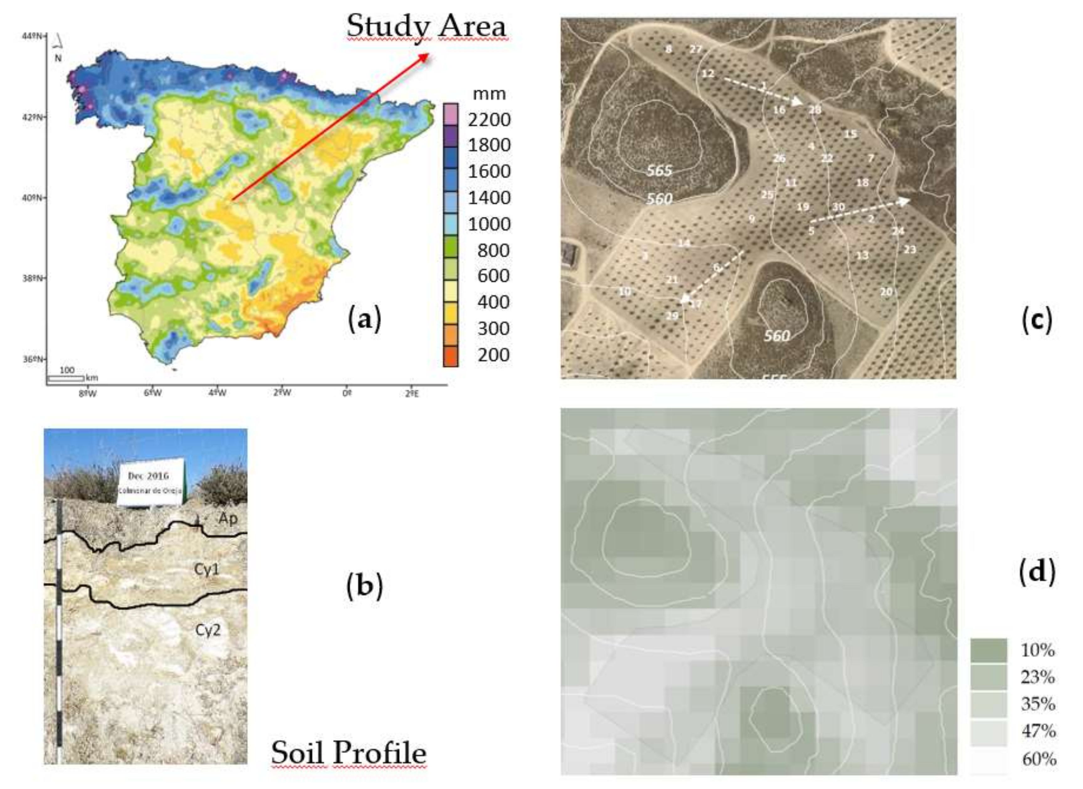
The study area is located in the south of Madrid (Datum ETRS89, latitude: 40°4′25′′ N; longitude: 3°31′20′′ W, Spain, Figure 1a). It is under Mediterranean semi-arid climatic conditions, with a mean annual temperature of 13.6 °C, accumulated annual precipitation of 380 mm and a reference evapo-transpiration (ET0 Penman-Monteith) of 1112 mm. Land use in this area is predominantly rain-fed woody cropping (vineyards and olive groves).
The plot under study is found in a rolling landscape, located between two hills with slopes between 12% and 14%, showing three different small watersheds with different orientations (Figure 1c). The sampling points were located between 540 and 560 m above sea level quite evenly distributed following a systematic random sampling design. The soils under study are described predominantly as Haplic Gypsisol in the low-lying areas [53] and as Gypsiric Regosol (WRB, 2014) in the higher lands. The study plot sized 3.7 ha hectares, shows mostly the later regosol type (Figure 1b), which includes shallow soils with Ap horizon being about 15 cm depth, with loamy texture and dry soil Munsell color 10YR 6/2, followed by Cy1 and Cy2 horizons with dry soil Munsell colors 10YR 7/2 and 10YR 8/1 respectively. Young olive trees were planted in this field in 2006 spaced 6 × 7 m and managed by minimum tillage up to 15–18 cm depth. Therefore, deeper layers were unaffected by chisel plow.
Thirty samples sites were selected to collect soil at three different depths (0 to 10, 10 to 20 and 20 to 30 cm; hereafter, 10, 20 and 30 depths), resulting in 90 soil samples. These 90 samples were air dried and sieved (2 mm) to collect fine earth and avoid artefacts due to roughness. Three subsamples were obtained to measure physical–chemical variables and to carry out the laboratory-based VIS/NIR spectral measurements.
2.2. Soil Analyses
Each one of the 90 samples was divided into three subsamples. The first set of subsamples was used to carry out laboratory methods to establish available water content (AWC), from field capacity (2.54 pF) to permanent wilting point (4.2 pF by the Richards plates method [54]; soil organic carbon content (g kg−1) by Loss On Ignition Method [55]). The SOC stock (Mg ha−1) was estimated using the recommendations given by the Intergovernmental Panel on Climate Change [56], which considers bulk density (Mg m−3) and soil thickness (m) following Equation (1), considering that there were no stones in the study area,
Stock = SOC (%) × Bulk density × depth × 100
The second set of subsamples was finely crushed and prepared for X-ray Diffraction analysis (XRD) in order to identify the type of minerals present in the soils [57]. The third set of subsamples was used for recording diffuse soil reflectance using ASD FieldSpecPro VIS/NIR (Analytical Spectral Devices Inc., Boulder, CO, USA) spectroradiometer, from 350 to 1100 nm with 3 nm VNIR spectral resolution. Scanning was performed in a dark room using the ASD contact probe provided with a halogen bulb with 2900 K color temperature, connected to the radiometer by an optical fiber; the contact probe was vertically placed in a pistol grip positioned on a tripod at 5 cm from the sample in order to minimize illumination differences. Soils samples dried at room temperature were placed on matte plastic black dishes (5 cm base diameter) so that they filled the dishes with 1 cm of soil thickness. A ruler was used to level the soil surface to guarantee a uniform sample. Each scan was an average of 10 internal scans to reduce random noise in the spectrum. In order to obtain the white reference or total reflectance, a standard Spectralon (Lab Sphere Inc., North Sutton, NH, USA) panel was used at the beginning of measurement and after each 10 min interval, always under the same illumination conditions. After checking the quality of spectra, noisy portions from 350 to 450 nm were removed before analysis. With the purpose of decreasing processing time, reducing over-parametrization for the model calibration and the number of predictors (independent variables), the soil spectra were averaged using a 10 nm window.
2.3. Statistical Analyses
The quantitative analysis of diffuse reflectance spectra was done by partial least squares regression (PLSR, [58]). The PLSR calculates successive orthogonal or latent factors to maximize the covariance of the predictor (X, the spectra) and response variables (Y, the soil parameters analyzed in the laboratory). This procedure avoids over-fitting or under-fitting choosing an optimum number of latent factors selected using the leave-one-out cross-validation. The procedure was carried out using the ParLes software version 3.1 [37]. The following soil variables were included for the spectral models: SOC, calcium carbonate, quartz, gypsum, illite, K-feldspars, Ca-K-feldspars, and phyllosilicates. Parts of the spectra were removed prior to performing PLSR analysis as they were considered insensitive or noisy [3]. In this study, spectra were considered from 450 to 1070 nm. The PLSR determined the best correlation between the spectral and the chemical data. The data were transformed in ParLeS software for normalizing, denoising and reducing non-linearities. Reflection data (R) were transformed to log (1/R) to reduce non-linearity. Normalization was performed using multiplicative signal correction (MSC) that corrects light scattering variations. The Savitzky–Golay filter was used to reduce random noise effects. Finally, background effects were removed using the first derivative of data, which indicates the slope of the spectral curve at every point [59] and minimizes grinding and optical set-up variations among samples [60].
Two-thirds of soil samples were randomly selected and used for model calibration (60 samples), and one third for validation (30 samples). As mentioned, leave-one-out cross-validation was performed to find the best latent variables, or factors, for the regression model [17], this implies that each successive calibration is made taking out one sample from the data set to build the regression model. No outliers were omitted from either calibration or validation datasets.
The accuracy of the cross validation was assessed by the root mean square error (RMSE; Equation (2))
where N is the sample size, yi’ is the predicted value and yi is the observed value.
The prediction ability of the model was estimated by calculating R2 statistics (0 < R2 < 1). The relative percent deviation (RPD; Equation (3)) that represents the ratio of the standard deviation of the y data to the RMSE of cross-validation predictions was used to determine the quality of predictions [61]. RPD < 1.4 indicates poor predictions; 1.4 < RPD < 1.8 indicates fair predictions, and RPD > 1.8 indicates very good predictions [3]. The optimum result will yield the highest R2, the lowest RMSE, and RPD > 1.4.
where SD is the standard deviation.
3. Results
3.1. Prediction of Physical–Chemical Properties
Statistic values of different parameters are listed in Table 1. The SOC content progressively decreases over depth and is reduced by half in 30 cm depth compared to the topsoil. Soils are characterized by a high content in gypsum, which is significantly higher at 30 cm depth. Calcium carbonate content is higher in upper soil layers up to 20 cm depth, and the same distribution is found for Illite. There are no significant differences in contents of quartz, phyllosilicates or feldspar between the three layers considered in this study.
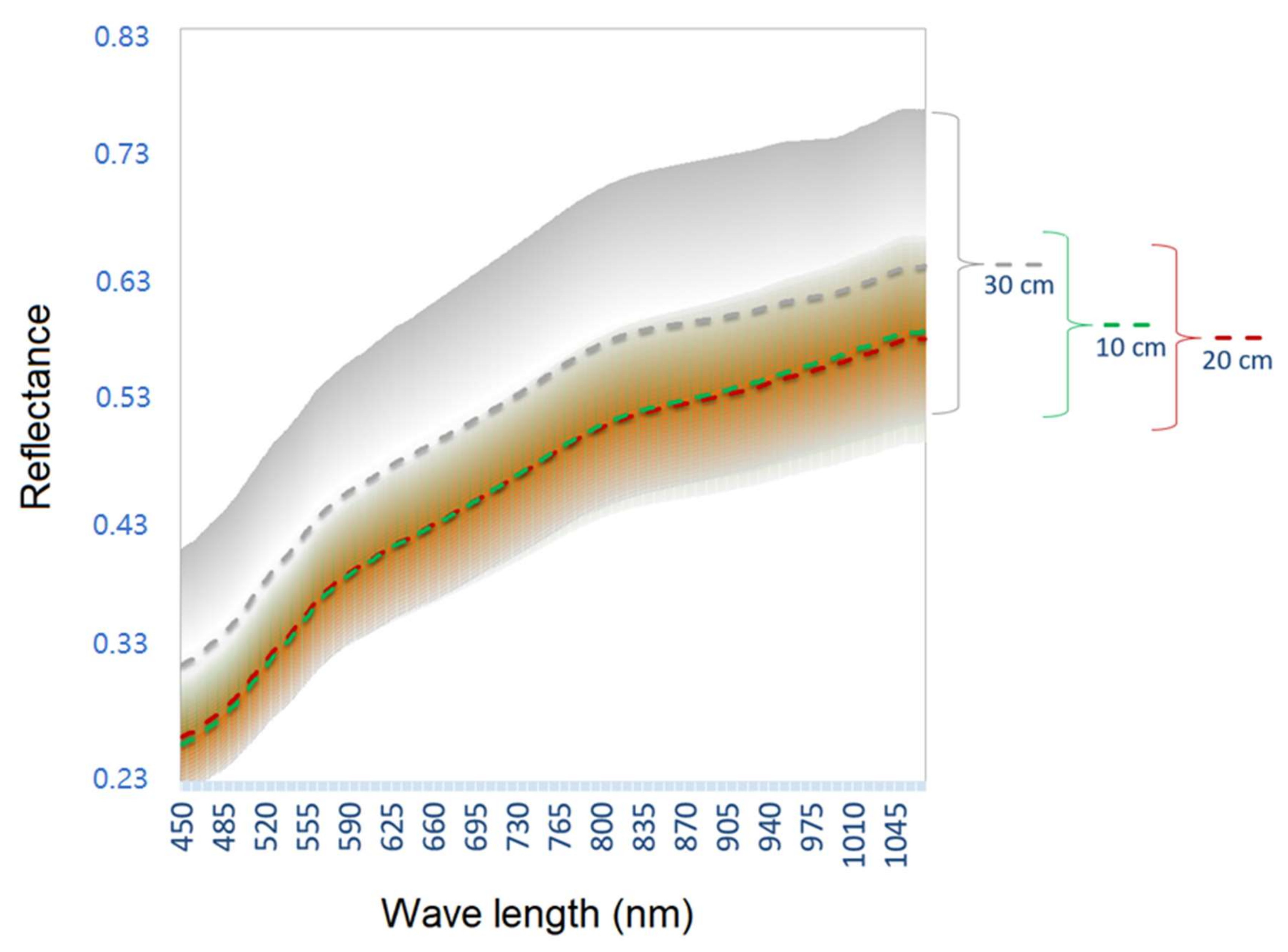
Soil diffuse reflectance mean and standard deviation of samples at three different depths are presented in Figure 2. As expected, minor features are shown in the visible and near-infrared portions of the spectrum [3]. In this study, soil spectrum signatures were not significantly different for the two first layers, which confirms physical–chemical data in Table 1. However, soils collected at 30 cm showed higher reflectance, higher gypsum and less SOC (Table 1). Lower SOC content lead to higher reflectance, which is frequent in drylands [35,62], especially when calcium carbonate and gypsum are abundant in soils [27]. Differences in soil reflectance of the plot of study can be observed by brightness index calculated from Sentinel 2 images (Figure 1d).
The VIS/NIR soil spectra were used to predict the physical–chemical properties in Table 1 using PLSR in ParLes software. As mentioned above, PLSR has been frequently used in chemometrics as it handles problems when there is a limited number of samples and many of them are correlated (Table 2). This set of samples showed that gypsum content was negatively correlated with the rest of the variables, which were, in turn, positively correlated between them, especially SOC. The highest correlations were found for illite and CaCO3.
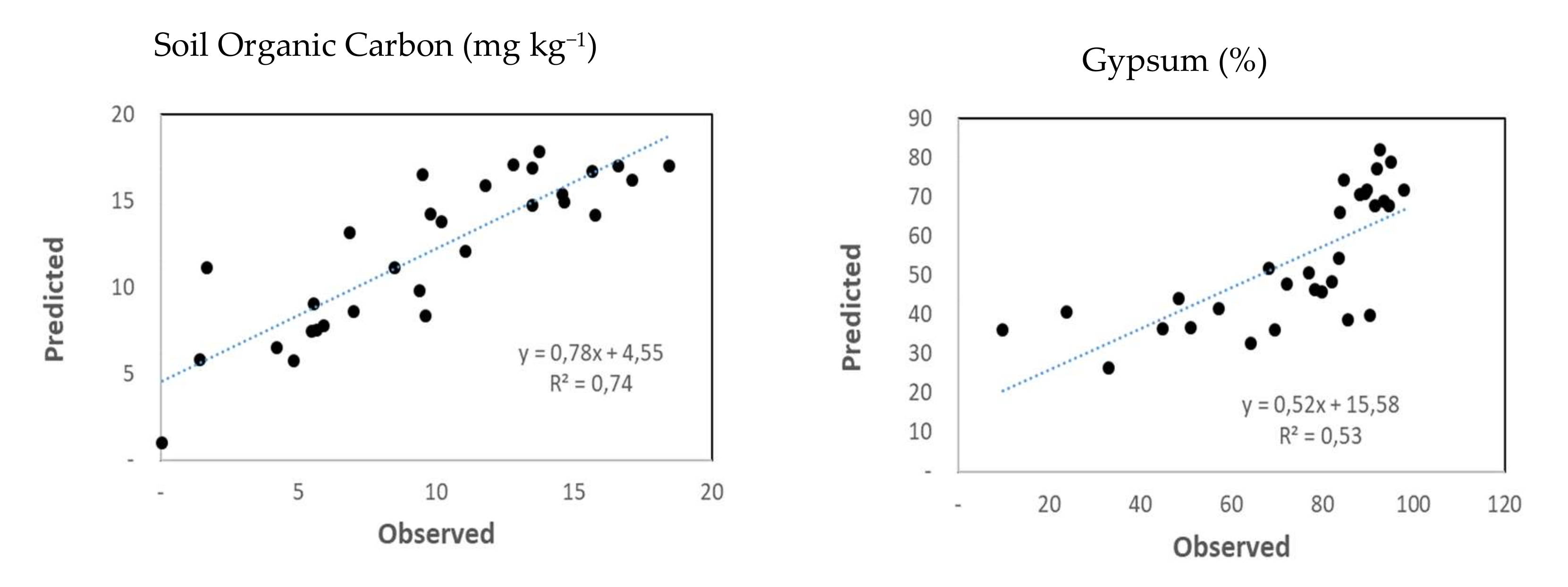
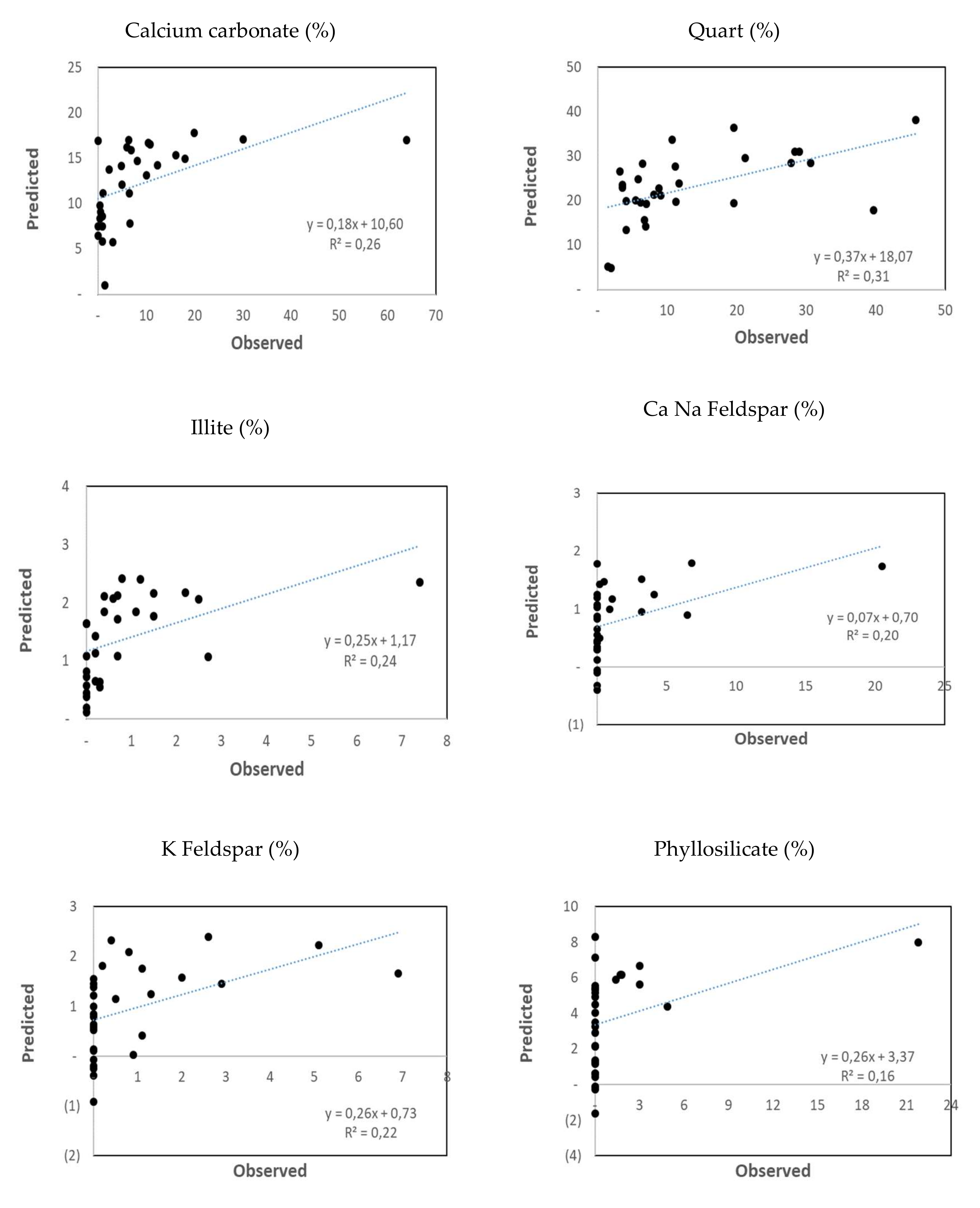
The calibration of ParLes software was performed with 60 randomly selected samples, and the validation with the remaining 30 samples. The cross-validation predictions of SOC produced an RMSE equal to 3.4 g kg−1; the R2 value was 0.74 (Table 3), which coincides with the average R2 reported for the visible range of the electromagnetic spectrum in a review gathering examples of SOC estimates from soil reflectance [42]. The statistics for predictions of the rest of the soil parameters were not considered accurate due to low R2 and RPD values. The observed versus predicted values for all the variables considered in the model are shown in Figure 3. Only SOC content showed a significant fit (R2 = 0.74), and fair quantitative predictions (RPD = 1.47). The second most important soil component that could be predicted by spectra was gypsum. According to the model, 53% of variations of gypsum can be explained by the model; however, RPD was 0.92 that can be considered without high accuracy.
3.2. Soil Organic Carbon and Available Water Capacity
The results of AWC are shown in Table 1. There was a significant difference in the soil moisture available for plants in the upper 10 cm of topsoil (gravimetric water content 12%), which was higher than AWC for layers underneath (between 6% and 9%). Importantly, there was a correlation between SOC content and available water for plants (Figure 4). The AWC showed a normal distribution with average 0.1 g g−1 and standard deviation 0.04 g g−1. Similarly, SOC average was 10.1 g kg−1 with a standard deviation 5.1 g kg−1. In general, topsoils (10 cm) showed higher SOC and AWC, and both variables decreased over depth. In these soils, 48% of variations of available water were explained by just SOC content, as other important factors such as clay content or soil structure were not considered for this model because previous research demonstrated that texture and structure in this area are fairly uniform [4].
4. Discussion
This study focused on degraded gypsiferous soils can be divided into two main objectives. First, to assess the potential use of VIS/NIR spectroscopy for the prediction of different soil components, especially SOC and gypsum, which are considered important indicators of soil conservation conditions. Second, to estimate the relationship between the previously emerged indicators and the ability of these soils to hold water.
Gypsiferous soils are usually found in regions with low precipitation and high evapotranspiration; in this central region of Spain, they are developed over gypsum deposits interbedded in marls, clays, and sandstones dating from the Lower Miocene [63]. They are characterized by a heterogeneous composition including gypsum, calcite, quartz, illite, kaolinite, and traces of palygorskite [64].
The procedure to determine or predict the chemical or mineralogical composition of soils using reflectance spectrometry is based on the overtone absorption and combination of bond vibrations in molecules of three functional groups in minerals: OH−, SO4−2, and CO3− [64,65]. The VIS, NIR and MIR ranges can be then used to assess soil properties simultaneously, but the choice of the particular spectral regions to be selected must be based on the balance between the accuracy of predictions, the cost of the technology and the sample preparation process [3].
As mentioned in the introduction, soil organic matter has been studied and accurately predicted using methods based on diffuse reflectance spectrometry. Different regions of the spectrum have been found to be appropriate for these goals. Other studies, using NIR and VIS range have reported R2 ranging from 0.53 [66] to 0.94 [67]. In this study, R2 was 0.74 using VIS/NIR range, therefore predictions are related to the height and slope of spectral signatures. This approach is considered cost-effective compared to other techniques covering a wider wavelength range [68].
The SOC content was low in these soils, which can be attributed to prolonged traditional tillage that started, at least partially, in 1975 [4]. The soil layers from 0–10 to 10–20 cm depth show similar reflectance features, and do not show significant differences between physical–chemical variables, due to the continuous tillage, which mixed the Ap horizon. Considering 30 cm depth as a whole, the SOC average content was 10.1 ± 5.1 g kg−1. In order to understand the magnitude of SOC loss, we can compare it with other figures found in gypsiferous soils of the same region not used for agriculture due to high stoniness and currently covered by oaks (Quercus ilex and Quercus coccifera) and herbaceous vegetation. These unused soils showed SOC content of 34.7 ± 2.6 g kg−1 [69]. Based on these figures, transformation of land use from forest to croplands results in 70% of SOC loss in this region. Such a difference makes SOC a powerful indicator of soil conservation or degradation.
Differences in albedo and slope in spectral signatures have been attributed to the variations in SOC content [35,70]. According to the model of this study, peaks that are important for SOC prediction in the gypsiferous soils of this study were found from 570 to 600 nm (green region) and from 990 to 1000 nm (NIR region). Viscarra Rosell et al., [3] found that visible range bands at 410, 570 and 660 nm showed good correlations with SOC. Daniel et al. [71] found a strong correlation between SOC and reflectance from approximately 960 to 1100 nm. The root mean square error and regression coefficients obtained from the PLRS analysis of this study showed that with three latent vectors selected, 74% of the variation of SOC content was explained by this model (R2 = 0.74), the RPD of 1.47 indicates an acceptable prediction, that could be improved using more samples. Conforti et al. [35] found more accurate predictions (R2 = 0.84; RPD = 2.53) in soils over gneiss and schists; other studies [72] show more similar results (R2 = 0.71; RPD = 1.84) for acid heterogeneous soils in the Central Amazon region. After searching for publications on the estimation of soil characteristics by VIS/NIR spectroscopy in gypsiferous areas, only a similar approach was found in the study of Babaeian et al. [73]. This research, located in Iran, demonstrated, by a stepwise multiple linear regression method, that SOC can be predicted by combinations of different wavelengths in the visible range (497, 677, 707, 772, and 797 nm) but also considering other wavelengths in NIR and MIR ranges, with an R2 = 0.69.
One of the aims of this study was the establishment of gypsum predictions. The model yielded moderate prediction features (R2 = 0.53; RPD = 0.92). However, XRD data showed a significant increase in gypsum concentration over depth that coincides with a decrease in SOC content. This fact was observed by other authors in gypsiferous areas, and lead them to establish that gypsum concentration, lack of SOC and high salts concentration can be considered as an index of desertification intensity [74]. Recent studies [52] have set up gypsum prediction in laboratory models using the Normalized Differenced Gypsum Index (NDGI) and the Half-Area and Continuum Removed Absorption Depth (CRAD) spectral parameters. These models yielded high prediction features R2 = 0.84 for NDGI and R2 = 0.86 for CRAD. Because of this, gypsum prediction functions have been applied to spaceborne imagery (Hyperion, airborne HySpex, or por EnMAP), being more suited for highly gypsiferous soils than for lower gypsiferous ones. This technological approach is not easily available to all laboratories. Further, sometimes hundreds or thousands of sets of less precise data are more useful than very few and very precise measurements [11]; this is of a special application when addressing sustainable land management in large areas. Independent research carried out in this area established that combinations of bands in true color images can be used to discriminate areas with high gypsum contents and little SOC [75]. In this study, a good correlation between visible wavelengths and gypsum content was established. This leads us to think that further work increasing the number of samples could yield more accurate results for gypsum.
Concerning the calcium carbonate content, its abundance was expected, as this component typically accumulates in semi-arid or arid environments. High contents of CaCO3 may act as a source of calcium due to its ease weathering, leading to mechanisms of flocculation and aggregation of soil particles; secondary CaCO3 minerals can be formed and help to increase cementing effects on soil aggregates [76] resulting in better structure and longer maintenance of SOC in mineral soils [77] that may explain the high correlation found with SOC. Calcium carbonate has been accurately predicted using PLSR techniques in the literature [70,78]. Though calcium carbonate is also an important component of these soils (median CaCO3 from 1.1% to 6.3%), the variability was remarkable, with values from 0% to 60%. In this region, CaCO3 and illite in topsoil come from the erosion of areas in the upper positions. Predictions for calcium carbonate are less accurate than predictions for gypsum in this area. Similar results were found on gypsiferous soils in Iran [51]. The rest of the compounds considered in this study—quartz, feldspars, etcetera—were even more variable or their concentrations were negligible. Thus, they were not appropriate for modeling and were not used as indicators of soil degradation or recovery.
The variations observed for SOC and gypsum contents indicated that in spite of an expected homogenization of soils throughout the plot by tillage, which was made two or three times a year, there were some differences between parts of the plot. These differences are due to the erosion processes that are imposed on the homogenization produced by tillage practices at a local level. The present approach, with samples taken from 0 to 10, 10 to 20 and 20 to 30 cm layers, is suitable for detailed analysis of erosion. These soils are affected by both water and tillage erosion as, in general, the sloped and upper positions show erosion-induced material losses, soils showed high reflectance with slight differences between the three layers considered, these soils are considered as severely degraded. On the contrary, soil samples at the flatter downslope areas tend to have higher SOC content and low albedo prevails, particularly for the upper soil layers. At the middle heights, intermediate situations regarding reflectance features were found. The irregular topography of the study plot introduced high variability in soil parameters; patterns based only on altitude were not consistent to determine soil changes. Further analyses are on the way to study the influence of other factors related to the proximity of channels; length from the top of the slope or aspect.
Sastre et al. [4] used the radioactive isotope 137Cs as an indicator of soil redistribution rates in this area and described that due to water and tillage erosion, 30 Mg ha−1 yr−1 of soils were lost in upper slope positions and, correspondingly, a deposition rate of c.a. 35 Mg ha−1 yr−1 was estimated at downslope positions; these figures included rill and interril erosion. According to these authors, soil organic matter and carbonate contents were double in downslope positions; they also found that Mg, K and P contents were also higher [4]. Long term effects of erosion lead to a progressive soil quality depletion that can be evidenced in the enrichment rate of SOC (SOC in sediments/SOC in soils) varying between 1.7 and 2.0 [79] in soils of the study area. The SOC content differences between eroded and depositional positions influenced the spectral signatures of these soils.
Carbon conservation in soils is becoming increasingly important in recent years, due to its central role in preventing and adapting ecosystems to climate change. International organizations such as the United Nations Framework Convention on Climate Change or the UN Convention to Combat Desertification, advocate for a comprehensive and rigorous study of the SOC stock changes using the IPCC guidelines for new management practices, with the aim to provide a sound scientific basis for future international climate action [5,80]. One of the purposes of this vision is the establishment of a starting point to study the evolution of the carbon stock over time. The SOC stock in the soils of this study was estimated using 30 cm depth, which was recommended by the IPCC as the reference depth. Soil bulk density was of 1.2 ± 0.2 Mg m−3 on average, therefore, the organic C stock in this sloping olive grove was on average 36.8 Mg ha−1. The minimum C stock was 2 Mg ha−1 (sample 4) and the maximum 60 Mg ha−1 (sample 30) corresponding to high and low topsoil reflectance respectively in the VIS/NIR regions. These figures are in line with data found in other Mediterranean regions, for example in vineyards (39,3 Mg ha−1) or olive groves (42.3 Mg ha−1) in South of Italy [81]; or C stocks of 28.79 Mg ha−1 in conventionally tilled soils in Central Morocco [82]. They are also in line with the results of an extensive research on carbon stocks in Spain, considering 30 cm depth, which states that stocks in woody crops are 38.09 ± 11.91 Mg C ha−1, however, far from the 150 Mg ha−1 in the cooler and wetter northern zones [83]. There is a potential for C sequestration in soils, if other sustainable land management practices different from frequent tillage are adopted, Gabarron-Galeote et al., [84] estimated this rate in 0.6 Mg ha−1 yr−1 in drylands in south Spain. Permanent cover crops between olive trees can increase SOC stock by 1 Mg ha−1 yr−1 in these gypsiferous soils during the first three years of management over 10 cm depth [85].
One remarkable consequence of SOC erosion and low levels of SOC stock is related to the loss of water availability. In this study, there was a significant relationship between SOC and AWC. In Table 1, we can see values grouped in lower and upper quartiles. Degraded soils can be grouped in the lower quartile of SOC contents, which contain 6.2 g of C per kilogram of soil; these soils hold, on average, 0.06 g of water per gram of soil, that is 21.6 L of water per square meter. These calculations involved bulk density, 1200 kg m−3, 0.3 m thickness = 360 kg soil m−2; 360 kg m−2 × 0.06 g g−1 = 21.6 kg or L m−2. Analogous calculations for non-eroded soils in this plot, which that can be grouped in the upper quartile of SOC content, contain in average SOC 14.0 g kg−1, and 0.14 g of water per g of soil, and then hold 50.4 L m−2 (360 kg of soil m−2 × 0.14 g g−1 = 50.4 kg or L m−2). The coefficients of variation of these figures ranged from c.a. 10% at the top soil and increase to 40% over depth.
Such a difference in water available for plants from 21.6 to 50.4 L per square meter can be used as an effective message to move land users to change into management practices aimed at increasing SOC content in agricultural soils. In this semiarid region, farmers perceive water as a priority [86], but not so the erosion processes [87] responsible for this situation. This is because farmers associate erosion only with extreme events and tend to ignore the long-term effects of unnoticed small losses [88]. One of the effects of maintained erosion rates, loss of SOC and lack of water availability is desertification [89]. This study provides a useful tool to monitor spatio-temporal changes by VIS/NIR satellite imagery that will help to prioritize policy measures to stop and prevent soil degradation.
5. Conclusions
Diffuse reflectance spectrometry (450–1050 nm) has been found to be a useful and cost-effective method to predict SOC content (R2 = 0.74; RPD = 1.47), especially in these soils with contrasting soil layers. There was a moderate prediction accuracy for gypsum content (R2 = 0.53; RPD = 0.92). The PLSR calibration and validation of models for other mineralogical components (CaCO3, quartz, feldspar, phyllosilicates or Illite) were not accurate in this study.
Tillage practices on sloping soils produce SOC mineralization and sediment loss, which is enriched in carbon and nutrients. In this study, it was estimated that 70% of SOC was lost in agricultural areas. In the three soil layers considered (10, 20 and 30 cm depth), the zones with low SOC also had low AWC. The upper sloped areas showed 7.18 g kg−1 SOC (lower quartile average) and had higher reflectance features in all three soil layers. Water content in these soils was estimated in 21.6 L m−2; conversely, downslope and flatter areas showed a higher SOC content, 14.0 g kg−1 (upper quartile average), showed lower reflectance features and held 50.4 L of water per square meter. Although these data show coefficients of variation of up to 40%, differences were significant. SOC accumulation can be an effective strategy for climate change adaptation in semi-arid areas as it is correlated to AWC.
Gypsum content increased significantly over depth and was negatively correlated with SOC. However, the increase in gypsum content in topsoil (0 to 10 cm) can be considered as an indicator of soil degradation, as this occurs in parallel to a decrease in SOC and AWC. Such a situation of eroded and degraded soils can be observed by remote sensing techniques. These cost-effective methods open the door for discrimination of degraded agricultural soils and further soil mapping of this area. This approach could be used for other similar gypsiferous soils after validation. As it meaningfully summarizes the state of these agricultural soils, it is relevant to environmental issues related to decision making, and also improves the communication of the extent and severity of land degradation to land users, policy makers, and other stakeholders.
Author Contributions
Individual contributions to the final version of this study were provided by M.J.M. and R.B. for conceptualization and draft preparation. All the co-authors, A.M.Á, P.C., I.E. and B.S. contributed to sampling, analytical procedures and review and edition works. All authors have read and agreed to the published version of the manuscript.
Funding
This research was funded by regional and national funding projects AGRISOST-CM (S2013/ABI-2717); FP12-CVO; ACCION Project, GO-LEÑOSOST.
Acknowledgments
We thank the staff of the Finca La Chimenea in Aranjuez for his help, we are also grateful to Jesús Galán and David Garrido, undergraduate students of Environmental Sciences in the Autonomous University of Madrid for their collaboration.
Conflicts of Interest
All the authors declare no conflict of interest.
Abbreviations
| AWC | available water content |
| C | Carbon |
| CRAD | Continuum Removed Absorption Depth |
| IPCC | Intergovernmental Panel on Climate Change |
| MSC | multiplicative signal correction |
| NDGI | Normalized Differenced Gypsum Index |
| PLSR | partial least square regression |
| RMSE | root mean square error |
| RPD | relative percent deviation |
| SD | where SD is the standard deviation |
| SOC | soil organic carbon |
| VIS/NIR | visible and near-infrared |
References
- Janik, L.J.; Merry, R.H.; Skjemstad, J.O. Can mid infrared diffuse reflectance analysis replace soil extractions? Aust. J. Exp. Agric. 1998, 38, 681–696. [Google Scholar] [CrossRef]
- Shepherd, K.D.; Walsh, M.G. Development of reflectance spectral libraries for characterization of soil properties. Soil Sci. Soc. Am. J. 2002, 66, 988–998. [Google Scholar] [CrossRef]
- Rossel, R.A.V.; Walvoort, D.J.J.; McBratney, A.B.; Janik, L.J.; Skjemstad, J.O. Visible, near infrared, mid infrared or combined diffuse reflectance spectroscopy for simultaneous assessment of various soil properties. Geoderma 2006, 131, 59–75. [Google Scholar] [CrossRef]
- Sastre, B. Estimating soil redistribution rates in an agricultural hillside by 137Cs: Case study in Central Spain on gypsiferous soil. In Empleo de Cubiertas vegetales en olivar, repercusión sobre el suelo, la erosión y la calidad del aceite de oliva virgen; Alcalá, U.D., Ed.; Universidad de Alcalá: Madrid, Spain, 2017; pp. 40–61. [Google Scholar]
- IPCC. Intergovernmental Panel on Climate Change Guidelines for National Greenhouse Gas Inventories; Eggleston, G.S., Miwa, K., Ngara, T., Tanabe, K., National Greenhouse Gas Inventories, Eds.; IGES: Kanagawa, Japan.
- Ben-Dor, E. Quantitative remote sensing of soil properties. Adv. Agron. 2002, 75, 173–243. [Google Scholar] [CrossRef]
- Ben-Dor, E.; Irons, J.R.; Epema, G.F. Soil reflectance. In Remote Sensing for the Earth Sciences: Manual of Remote Sensing; Rencz, N., Ed.; John Wiley & Sons: New York, NY, USA, 1999; Volume 3. [Google Scholar]
- Fernandes, R.B.A.; Barron, V.; Torrent, J.; Fontes, M.P.F. Quantification of iron oxides in Brazilian latosols by diffuse reflectance spectroscopy. Revista Brasileira De Ciencia Do Solo 2004, 28, 245–257. [Google Scholar] [CrossRef]
- Reeves, J.B. Near-versus mid-infrared diffuse reflectance spectroscopy for soil analysis emphasizing carbon and laboratory versus on-site analysis: Where are we and what needs to be done? Geoderma 2010, 158, 3–14. [Google Scholar] [CrossRef]
- Bellon-Maurel, V.; McBratney, A. Near-infrared (NIR) and mid-infrared (MIR) spectroscopic techniques for assessing the amount of carbon stock in soils—Critical review and research perspectives. Soil Biol. Biochem. 2011, 43, 1398–1410. [Google Scholar] [CrossRef]
- McBratney, A.B.; Minasny, B.; Rossel, R.V. Spectral soil analysis and inference systems: A powerful combination for solving the soil data crisis. Geoderma 2006, 136, 272–278. [Google Scholar] [CrossRef]
- Waiser, T.H.; Morgan, C.L.S.; Brown, D.J.; Hallmark, C.T. In situ characterization of soil clay content with visible near-infrared diffuse reflectance spectroscopy. Soil Sci. Soc. Am. J. 2007, 71, 389–396. [Google Scholar] [CrossRef]
- Clark, R.N. Spectroscopy of rocks and minerals and principles of spectroscopy. In Remote Sensing for the Earth Sciences: Manual of Remote Sensing; Rencz, N., Ed.; Johng Wiley & Sons: New York, NY, USA, 1999; Volume 3. [Google Scholar]
- Rossel, R.A.V.; Webster, R. Predicting soil properties from the Australian soil visible-near infrared spectroscopic database. Eur. J. Soil Sci. 2012, 63, 848–860. [Google Scholar] [CrossRef]
- Guerrero, C.; Mataix-Solera, J.; Arcenegui, V.; Mataix-Beneyto, J.; Gomez, I. Near-infrared spectroscopy to estimate the maximum temperatures reached on burned soils. Soil Sci. Soc. Am. J. 2007, 71, 1029–1037. [Google Scholar] [CrossRef]
- Sorensen, L.K.; Dalsgaard, S. Determination of clay and other soil properties by near infrared spectroscopy. Soil Sci. Soc. Am. J. 2005, 69, 159–167. [Google Scholar] [CrossRef]
- Reeves, J.B.; McCarty, G.W.; Reeves, V.B. Mid-infrared diffuse reflectance spectroscopy for the quantitative analysis of agricultural soils. J. Agric. Food Chem. 2001, 49, 766–772. [Google Scholar] [CrossRef] [PubMed]
- Udelhoven, T.; Emmerling, C.; Jarmer, T. Quantitative analysis of soil chemical properties with diffuse reflectance spectrometry and partial least-square regression: A feasibility study. Plant Soil 2003, 251, 319–329. [Google Scholar] [CrossRef]
- Brown, D.J.; Shepherd, K.D.; Walsh, M.G.; Mays, M.D.; Reinsch, T.G. Global soil characterization with VNIR diffuse reflectance spectroscopy. Geoderma 2006, 132, 273–290. [Google Scholar] [CrossRef]
- Pirie, A.; Singh, B.; Islam, K. Ultra-violet, visible, near-infrared, and mid-infrared diffuse reflectance spectroscopic techniques to predict several soil properties. Aust. J. Soil Res. 2005, 43, 713–721. [Google Scholar] [CrossRef]
- Minasny, B.; McBratney, A.B.; Tranter, G.; Murphy, B.W. Using soil knowledge for the evaluation of mid-infrared diffuse reflectance spectroscopy for predicting soil physical and mechanical properties. Eur. J. Soil Sci. 2008, 59, 960–971. [Google Scholar] [CrossRef]
- Rossel, R.A.V.; Behrens, T.; Ben-Dor, E.; Brown, D.J.; Dematte, J.A.M.; Shepherd, K.D.; Shi, Z.; Stenberg, B.; Stevens, A.; Adamchuk, V.; et al. A global spectral library to characterize the world’s soil. Earth Sci. Rev. 2016, 155, 198–230. [Google Scholar] [CrossRef] [Green Version]
- De Jong, S.M. Applications of Reflective Remote Sensing for Land Degradation Studies in a Mediterranean Environment; The royal Dutch Geographical Society; Faculty of Geographical Sciences: Utrecht, The Netherlands, 1994; p. 260. [Google Scholar]
- Leone, A.P.; Sommer, S. Multivariate analysis of laboratory spectra for the assessment of soil development and soil degradation in the southern Apennines (Italy). Remote Sens. Environ. 2000, 72, 346–359. [Google Scholar] [CrossRef]
- De Jong, S.M. Imaging spectrometry for surveying and modelling land degradation. In Imaging Spectrometry; van der Meer, F.D., de Jong, S.M., Eds.; Kluwer Academic Publishers: Dordrecht, The Netherlands, 2001; pp. 65–86. [Google Scholar]
- Dematte, J.A.M.; Campos, R.C.; Alves, M.C.; Fiorio, P.R.; Nanni, M.R. Visible-NIR reflectance: A new approach on soil evaluation. Geoderma 2004, 121, 95–112. [Google Scholar] [CrossRef]
- Shrestha, D.P.; Margate, D.E.; van der Meer, F.; Anh, H.V. Analysis and classification of hyperspectral data for mapping land degradation: An application in southern Spain. Int. J. Appl. Earth Obs. Geoinf. 2005, 7, 85–96. [Google Scholar] [CrossRef]
- Cecillon, L.; Cassagne, N.; Czarnes, S.; Gros, R.; Vennetier, M.; Brun, J.J. Predicting soil quality indices with near infrared analysis in a wildfire chronosequence. Sci. Total Environ. 2009, 407, 1200–1205. [Google Scholar] [CrossRef] [PubMed] [Green Version]
- Kemper, T.; Sommer, S. Estimate of heavy metal contamination in soils after a mining accident using reflectance spectroscopy. Environ. Sci. Technol. 2002, 36, 2742–2747. [Google Scholar] [CrossRef] [PubMed]
- Farifteh, J.; Van der Meer, F.D.; Atzberger, C.; Carranza, E.J.M. Quantitative analysis of salt-affected soil reflectance spectra: A comparison of two adaptive methods (PLSR and ANN). Remote Sens. Environ. 2007, 110, 59–78. [Google Scholar] [CrossRef]
- Metternicht, G.I.; Zinck, J.A. Remote sensing of soil salinity: Potentials and constraints. Remote Sens. Environ. 2003, 85, 1–20. [Google Scholar] [CrossRef]
- Latz, K.; Weismiller, R.A.; Vanscoyoc, G.E.; Baumgardner, M.F. Characteristic variations in spectral reflectance of selected eroded alfisols. Soil Sci. Soc. Am. J. 1984, 48, 1130–1134. [Google Scholar] [CrossRef]
- Weissmiller, R.A.; VanScoyoc, G.E.; Pazar, S.E.; Latz, K.; Baumgardner, M.F. Use of soil spectral properties for monitoring soil erosion. In Soil Erosion and Conservation; Soil and Water Conservation Society of America: Ankeny, IA, USA, 1985; pp. 119–127. [Google Scholar]
- De Graffenried, J.B.; Shepherd, K.D. Rapid erosion modeling in a Western Kenya watershed using visible near infrared reflectance, classification tree analysis and (137) Cesium. Geoderma 2009, 154, 93–100. [Google Scholar] [CrossRef] [Green Version]
- Conforti, M.; Buttafuoco, G.; Leone, A.P.; Aucelli, P.P.C.; Robustelli, G.; Scarciglia, F. Studying the relationship between water-induced soil erosion and soil organic matter using Vis-NIR spectroscopy and geomorphological analysis: A case study in southern Italy. Catena 2013, 110, 44–58. [Google Scholar] [CrossRef]
- Krishnan, P.; Alexander, J.D.; Butler, B.J.; Hummel, J.W. Reflectance technique for predicting soil organic-matter. Soil Sci. Soc. Am. J. 1980, 44, 1282–1285. [Google Scholar] [CrossRef]
- Gomez, C.; Rossel, R.A.V.; McBratney, A.B. Comparing predictions of soil organic carbon by field Vis-NIR Spectroscopy and hyper spectral remote sensing. Geophys. Res. Abstr. 2008, 10, 1–2. [Google Scholar]
- Stevens, A.; Udelhoven, T.; Denis, A.; Tychon, B.; Lioy, R.; Hoffmann, L.; van Wesemael, B. Measuring soil organic carbon in croplands at regional scale using airborne imaging spectroscopy. Geoderma 2010, 158, 32–45. [Google Scholar] [CrossRef]
- Vasques, G.M.; Grunwald, S.; Sickman, J.O. Modeling of Soil Organic Carbon Fractions Using Visible–Near-Infrared Spectroscopy. Soil Sci. Soc. Am. J. 2009, 73, 176–184. [Google Scholar] [CrossRef] [Green Version]
- Reeves, J.; McCarty, G.; Mimmo, T. The potential of diffuse reflectance spectroscopy for the determination of carbon inventories in soils. Environ. Pollut. 2002, 116, S277–S284. [Google Scholar] [CrossRef]
- Stevens, A.; van Wesemael, B.; Bartholomeus, H.; Rosillon, D.; Tychon, B.; Ben-Dor, E. Laboratory, field and airborne spectroscopy for monitoring organic carbon content in agricultural soils. Geoderma 2008, 144, 395–404. [Google Scholar] [CrossRef] [Green Version]
- Ladoni, M.; Bahrami, H.A.; Alavipanah, S.K.; Norouzi, A.A. Estimating soil organic carbon from soil reflectance: A review. Precis. Agric. 2010, 11, 82–99. [Google Scholar] [CrossRef]
- Nettleton, W.D.; Nelson, R.E.; Brasher, B.R.; Derr, P.S. Gypsiferous soils in the Western United States. In Acid Sulfate Weathering; SSSA: Madison, WI, USA, 1982; Volume 10, pp. 147–168. [Google Scholar]
- Herrero, J.; Artieda, O.; Hudnall, W.H. Gypsum, a Tricky Material. Soil Sci. Soc. Am. J. 2009, 73, 1757–1763. [Google Scholar] [CrossRef]
- Poch, R.M.; De Coster†, W.; Stoops, G. Pore space characteristics as indicators of soil behaviour in gypsiferous soils. Geoderma 1998, 87, 87–109. [Google Scholar] [CrossRef]
- Etesami, H.; Halajian, L.; Jamei, M. A qualitative land suitability assessment in gypsiferous soils of Kerman Provicen, Iran. Aust. J. Basic Appl. Sci. 2012, 6, 60–64. [Google Scholar]
- Moret-Fernandez, D.; Herrero, J. Effect of gypsum content on soil water retention. J. Hydrol. 2015, 528, 122–126. [Google Scholar] [CrossRef] [Green Version]
- Smith, R.; Robertson, V.C. Soil and irrigation classification of shallow soils overlying gypsum beds, northern Iraq. J. Soil Sci. 1962, 13, 106–115. [Google Scholar] [CrossRef]
- Shrestha, D.P.; Zinck, J.A. Land use classification in mountainous areas: Integration of image processing, digital elevation data and field knowledge (application to Nepal). Int. J. Appl. Earth Obs. Geoinf. 2001, 3, 78–85. [Google Scholar] [CrossRef]
- Castroviejo, S.; Porta, J. Apport a l’écologie de la végétation des zones saltes des rives de la Gigtiela (Ciudad Real-Espagne). Les vases salées, Colloques phytosociologiques de Lille 1975, 4, 115–139. [Google Scholar]
- Khayamim, F.; Wetterlind, J.; Khademi, H.; Robertson, A.H.J.; Cano, A.F.; Stenberg, B. Using Visible and near Infrared Spectroscopy to Estimate Carbonates and Gypsum in Soils in Arid and Subhumid Regions of Isfahan, Iran. J. Near Infrared Spectrosc. 2015, 23, 155–165. [Google Scholar] [CrossRef] [Green Version]
- Milewski, R.; Chabrillat, S.; Brell, M.; Schleicher, A.M.; Guanter, L. Assessment of the 1.75 mu m absorption feature for gypsum estimation using laboratory, air- and spaceborne hyperspectral sensors. Int. J. Appl. Earth Obs. Geoinf. 2019, 77, 69–83. [Google Scholar] [CrossRef]
- Sastre, B.; Bienes, R.; Garcia-Diaz, A. How much is soil volumetric water content influenced by cover crops in an olive grove in central Spain? In VIII International Olive Symposium; Perica, S., Selak, G.V., Klepo, T., Ferguson, L., Sebastiani, L., Eds.; ISHS: Split, Croatia, 2016; Volume 1199, pp. 345–350. [Google Scholar]
- Richards, L.A. A pressure-membrane extraction apparatus for soil solution. Soil Sci. 1941, 51, 377–386. [Google Scholar] [CrossRef]
- Schulte, E.E.; Hopkins, B.G. Estimation of Organic Matter by Weight Loss-on-Ignition. In Soil Organic Matter: Analysis and Interpretation; Magdoff, F.R., Tabatabai, M.A., Hanlon, E.A., Jr., Eds.; SSSA Special Publication: Madison, WI, USA, 1996; pp. 21–31. [Google Scholar]
- Penman, J.; Gytarsky, M.; Hiraishi, T.; Krug, T.; Kruger, D.; Pipatti, R.; Buendia, L.; Miwa, K.; Ngara, T.; Tanabe, K.; et al. Section 3. LUCF Sector Good Practice Guidance. In Good Practice Guidance for Land Use, Land-Use Change and Forestry; IPCC National Greenhouse Gas Inventories Programme; Institute for Global Environmental Strategies (IGES): Hayama, Kanagawa, Japan, 2003; pp. 3.1–3.312. Available online: https://www.ipcc.ch/site/assets/uploads/2018/03/GPG_LULUCF_FULLEN.pdf (accessed on 16 January 2020).
- Klug, H.P.; Alexander, L.E. X-ray Diffraction Procedures for Polycrystalline and Amorphous Materials, 2nd ed.; Wiley: New York, NY, USA, 1974. [Google Scholar]
- Wold, H. Systems Analysis by Partial Least Squares. In IIASA Collaborative Paper; IIASA: Laxenburg, Austria, 1983. [Google Scholar]
- Kariuki, P.C.; Woldai, T.; Meer, F.V.D. Effectiveness of spectroscopy in identification of swelling indicator clay minerals. Int. J. Remote Sens. 2004, 25, 455–469. [Google Scholar] [CrossRef]
- Martens, H.; Naes, T. Multivariate Calibration; Wiley: Chichester, UK, 1989. [Google Scholar]
- Chang, C.-W.; Laird, D.A. Near-infrared reflectance spectroscopic analysis of soil C and N. Soil Sci. 2002, 167, 110–116. [Google Scholar] [CrossRef]
- Tola, E.; Al-Gaadi, K.A.; Madugundu, R.; Kayad, A.G.; Alameen, A.A.; Edrees, H.F.; Edriss, M.K. Determination of soil organic carbon concentration in agricultural fields using a handheld spectroradiometer: Implication for soil fertility measurement. Int. J. Agric. Biol. Eng. 2018, 11, 13–19. [Google Scholar] [CrossRef] [Green Version]
- Van Alpen, J.G.; de los Ríos-Romero, F. Gypsiferous soils. Notes on Their Characteristics and Management; International Institute for Land Reclamation and Improvement: Wageningen, The Netherlands, 1971; p. 44. [Google Scholar]
- Gumuzzio, J.; Casas, J. Accumulations of soluble salts and gypsum in soils of the Central Region, Spain. Cahiers ORSTOM. Série Pédologie 1988, 24, 215–226. [Google Scholar]
- Ben-Dor, E.; Banin, A. Near-Infrared Analysis as a Rapid Method to Simultaneously Evaluate Several Soil Properties. Soil Sci. Soc. Am. J. 1995, 59, 364–372. [Google Scholar] [CrossRef]
- Palacios-Orueta, A.; Ustin, S.L. Remote Sensing of Soil Properties in the Santa Monica Mountains I. Spectral Analysis. Remote Sens. Environ. 1998, 65, 170–183. [Google Scholar] [CrossRef]
- Reeves, J.B.; McCarty, G.W. Quantitative analysis of agricultural soils using near infrared reflectance spectroscopy and a fibre-optic probe. J. Near Infrared Spectrosc. 2001, 9, 25–34. [Google Scholar] [CrossRef]
- Melendez-Pastor, I.; Navarro-Pedreño, J.; Gómez, I.; Koch, M. Identifying optimal spectral bands to assess soil properties with VNIR radiometry in semi-arid soils. Geoderma 2008, 147, 126–132. [Google Scholar] [CrossRef]
- Barbero-Sierra, C.; Perez, M.R.; Perez, M.J.M.; Gonzalez, A.M.A.; Macein, J.L.C. Local and scientific knowledge to assess plot quality in Central Spain. Arid Land Res. Manag. 2018, 32, 111–129. [Google Scholar] [CrossRef]
- Summers, D.; Lewis, M.; Ostendorf, B.; Chittleborough, D. Visible near-infrared reflectance spectroscopy as a predictive indicator of soil properties. Ecol. Indic. 2011, 11, 123–131. [Google Scholar] [CrossRef]
- Daniel, K.W.; Tripathi, N.K.; Honda, K.; Apisit, E. Analysis of VNIR (400-1100 nm) spectral signatures for estimation of soil organic matter in tropical soils of Thailand. Int. J. Remote Sens. 2004, 25, 643–652. [Google Scholar] [CrossRef]
- Pinheiro, E.F.M.; Ceddia, M.B.; Clingensmith, C.M.; Grunwald, S.; Vasques, G.M. Prediction of Soil Physical and Chemical Properties by Visible and Near-Infrared Diffuse Reflectance Spectroscopy in the Central Amazon. Remote Sens. 2017, 9. [Google Scholar] [CrossRef] [Green Version]
- Babaeian, E.; Homaee, M.; Vereecken, H.; Montzka, C.; Norouzi, A.A.; van Genuchten, M.T. A Comparative Study of Multiple Approaches for Predicting the Soil-Water Retention Curve: Hyperspectral Information vs. Basic Soil Properties. Soil Sci. Soc. Am. J. 2015, 79, 1043–1058. [Google Scholar] [CrossRef] [Green Version]
- Khanamani, A.; Fathizad, H.; Karimi, H.; Shojaei, S. Assessing desertification by using soil indices. Arab. J. Geosci. 2017, 10. [Google Scholar] [CrossRef]
- García-Rodríguez, M.P.; Pérez-González, M.E. Discriminación de gypsisoles mediante el sensor ETM+ del satélite LANDSAT-7. Edafología 2001, 8, 25–36. [Google Scholar]
- Rowley, M.C.; Grand, S.; Verrecchia, E.P. Calcium-mediated stabilisation of soil organic carbon. Biogeochemistry 2018, 137, 27–49. [Google Scholar] [CrossRef] [Green Version]
- Fernandez-Ugalde, O.; Virto, I.; Barre, P.; Gartzia-Bengoetxea, N.; Enrique, A.; Imaz, M.J.; Bescansa, P. Effect of carbonates on the hierarchical model of aggregation in calcareous semi-arid Mediterranean soils. Geoderma 2011, 164, 203–214. [Google Scholar] [CrossRef]
- Volkan Bilgili, A.; van Es, H.M.; Akbas, F.; Durak, A.; Hively, W.D. Visible-near infrared reflectance spectroscopy for assessment of soil properties in a semi-arid area of Turkey. J. Arid Environ. 2010, 74, 229–238. [Google Scholar] [CrossRef]
- Ruiz-Colmenero, M.; Bienes, R.; Marques, M.J. Soil and water conservation dilemmas associated with the use of green cover in steep vineyards. Soil Tillage Res. 2011, 117, 211–223. [Google Scholar] [CrossRef]
- Orr, B.J.; Cowie, A.L.; Castillo Sanchez, V.M.; Chasek, P.; Crossman, N.D.; Erlewein, A.; Louwagie, G.; Maron, M.; Metternicht, G.I.; Minelli, S.; et al. Scientific Conceptual Framework for Land Degradation Neutrality. A Report of the Science-Policy Interface. Available online: http://www2.unccd.int/sites/default/files/documents/LDNScientificConceptualFramework_FINAL.pdf (accessed on 1 November 2019).
- Farina, R.; Di Bene, C.; Francaviglia, R.; Napoli, R.; Marchetti, A. Towards a tier 3 approach to estimate SOC stocks at sub-regional scale in sourhern Italy. In Proceedings of the Global Symposium on Soil Organic Carbon, Rome, Italy, 21–23 March 2017; pp. 72–75. [Google Scholar]
- Moussadek, R.; Mrabet, R. Carbon management and sequestration in dryalnd soils of Morocco: Nexus approach. In Proceedings of the Global Symposium on Soil Organic Carbon, Rome, Italy, 21–23 March 2017; pp. 497–500. [Google Scholar]
- Martin, J.A.R.; Alvaro-Fuentes, J.; Gonzalo, J.; Gil, C.; Ramos-Miras, J.J.; Corbi, J.M.G.; Boluda, R. Assessment of the soil organic carbon stock in Spain. Geoderma 2016, 264, 117–125. [Google Scholar] [CrossRef] [Green Version]
- Gabarron-Galeore, M.A.; Trigalet, S.; van Wesemael, B. Soil organic carbon evolution after land abandonment along a precipitation gradient in southern Spain. Agric. Ecosyst. Environ. 2015, 199, 114–123. [Google Scholar] [CrossRef]
- Sastre, B.; Marques, M.J.; Garcia-Diaz, A.; Bienes, R. Three years of management with cover crops protecting sloping olive groves soils, carbon and water effects on gypsiferous soil. Catena 2018, 171, 115–124. [Google Scholar] [CrossRef]
- Barbero-Sierra, C.; Marques, M.J.; Ruiz-Perez, M.; Bienes, R.; Cruz-Macein, J.L. Farmer knowledge, perception and management of soils in the Las Vegas agricultural district, Madrid, Spain. Soil Use Manag. 2016, 32, 446–454. [Google Scholar] [CrossRef]
- Marques, M.J.; Bienes, R.; Cuadrado, J.; Ruiz-Colmenero, M.; Barbero-Sierra, C.; Velasco, A. Analysing Perceptions Attitudes and Responses of Winegrowers about Sustainable Land Management in Central Spain. Land Degrad. Dev. 2015, 26, 458–467. [Google Scholar] [CrossRef]
- Brunner, A.C.; Park, S.J.; Ruecker, G.R.; Vlek, P.L.G. Erosion modelling approach to simulate the effect of land management options on soil loss by considering catenary soil development and farmers perception. Land Degrad. Dev. 2008, 19, 623–635. [Google Scholar] [CrossRef]
- Angelakis, A.; Kosmas, C. Water resources availability in relation to the threat for further degradation in the Mediterranean region: Need for qualitative and qualitative indicators. In Proceedings of the Indicators for Assessing Desertification in the Mediterranean. Proceedings of the International Seminar, Porto Torres, Italy, 18–20 September 1998; pp. 52–65. [Google Scholar]
Figure 1.
Location of study. (a) Spain Map source: National Agency Meteorology; (b) soil profile; (c) sampling sites; (d) Brightness Index = sqrt(B82 + B42 + B32), obtained from VIS/NIR bands of cloud-free Sentinel-2 image, acquired on 15 November 2017 and downloaded from ESA Sentinels Scientific Data-Hub.

Figure 2.
Soil reflectance, VIS/NIR range (4050–1050 nm). Average (short-dashed lines) and standard deviation of samples from 10, 20 and 30 cm depth in brackets on the right (n = 30).
Figure 2.
Soil reflectance, VIS/NIR range (4050–1050 nm). Average (short-dashed lines) and standard deviation of samples from 10, 20 and 30 cm depth in brackets on the right (n = 30).

Figure 3.
Cross-validation results of ParLeS software for soil physical–chemical variables. Observed versus predicted values.
Figure 3.
Cross-validation results of ParLeS software for soil physical–chemical variables. Observed versus predicted values.


Figure 4.
Cross-validation results of ParLeS software for soil physical–chemical variables. Observed versus predicted values.
Figure 4.
Cross-validation results of ParLeS software for soil physical–chemical variables. Observed versus predicted values.


Table 1.
Descriptive statistics of physical chemical soil variables. N = 30 samples per depth. Global set of samples = 90 (30 samples × three depths). The available water capacity (AWC) indicates water content in field capacity minus water content in permanent wilting point. Different letters indicate significant differences (p < 0.05) between depths. Kruskal–Wallis test.
| Soil Property | Depth (cm) | Median | Minimum | Maximum | Lower Quartile | Upper Quartile |
|---|---|---|---|---|---|---|
| SOC (g kg−1) | 10 | 12.35 a | 0.80 | 20.81 | 10.19 | 16.60 |
| 20 | 9.85 a | 0.45 | 18.46 | 8.02 | 14.58 | |
| 30 | 5.80 b | 0.05 | 17.20 | 3.33 | 11.22 | |
| 30 cm range (Mean ± SD) | 10.1 ± 5.1 | 6.2 | 14.0 | |||
| C Stock (Mg ha−1) | 10 | 44.6 a | 3.0 | 76.4 | 31.6 | 58.4 |
| 20 | 36.4 a | 1.6 | 71.7 | 28.1 | 45.0 | |
| 30 | 25.7 b | 0.2 | 71.1 | 14.1 | 45.0 | |
| 30 cm range (Mean ± SD) | 36.8 ± 18.6 | 25.2 | 50.1 | |||
| Gypsum (%) | 10 | 81.6 a | 12.4 | 95.1 | 69.6 | 88.5 |
| 20 | 80.0 a | 3.1 | 94.6 | 59.3 | 89.6 | |
| 30 | 85.6 b | 3.1 | 97.9 | 48.1 | 93.2 | |
| 30 cm range (Mean ± SD) | 72.5 ± 23.9 | 63.2 | 90.2 | |||
| CaCO3 (%) | 10 | 6.3 a | 0.5 | 58.0 | 3.7 | 11.4 |
| 20 | 5.7 a | 0.2 | 63.9 | 2.5 | 12.4 | |
| 30 | 1.1 b | 0.0 | 57.7 | 0.5 | 8.7 | |
| 30 cm range (Mean ± SD) | 9.5 ± 12.9 | 1.0 | 11.4 | |||
| Quartz (%) | 10 | 9.8 a | 2.8 | 29.1 | 5.8 | 16.4 |
| 20 | 8.6 a | 3.3 | 37.9 | 4.4 | 19.6 | |
| 30 | 8.2 a | 1.5 | 56.5 | 5.6 | 22.2 | |
| 30 cm range (Mean ± SD) | 13.6 ± 11.6 | 5.3 | 18.8 | |||
| Illite (%) | 10 | 0.38 a | 0.00 | 4.56 | 0.00 | 0.85 |
| 20 | 0.57 a | 0.00 | 4.47 | 0.21 | 1.07 | |
| 30 | 0.00 b | 0.00 | 7.37 | 0.00 | 0.68 | |
| 30 cm range (Mean ± SD) | 0.78 ± 1.23 | 0.00 | 0.90 | |||
| Ca-Na Feldspar (%) | 10 | 0.00 a | 0.00 | 5.98 | 0.00 | 0.28 |
| 20 | 0.09 a | 0.00 | 6.75 | 0.00 | 1.33 | |
| 30 | 0.00 a | 0.00 | 20.47 | 0.00 | 0.45 | |
| 30 cm range (Mean ± SD) | 0.92 ± 2.54 | 0.00 | 0.74 | |||
| K-Feldspar (%) | 10 | 0.00 a | 0.00 | 8.69 | 0.00 | 0.85 |
| 20 | 0.42 a | 0.00 | 7.57 | 0.00 | 0.94 | |
| 30 | 0.00 a | 0.00 | 9.02 | 0.00 | 0.00 | |
| 30 cm range (Mean ± SD) | 0.85 ± 1.8 | 0.00 | 0.82 | |||
| Phyllosilicate (%) | 10 | 0.00 a | 0.00 | 22.10 | 0.00 | 1.42 |
| 20 | 0.00 a | 0.00 | 20.70 | 0.00 | 1.80 | |
| 30 | 0.00 a | 0.00 | 21.83 | 0.00 | 1.68 | |
| 30 cm range (Mean ± SD) | 1.78 ± 4.46 | 0.00 | 1.68 | |||
| WAC (g g−1) | 10 | 0.12 a | 0.07 | 0.17 | 0.10 | 0.15 |
| 20 | 0.09 b | 0.02 | 0.19 | 0.06 | 0.13 | |
| 30 | 0.06 b | 0.01 | 0.20 | 0.05 | 0.09 | |
| 30 cm range (Mean ± SD) | 0.10 ± 0.05 | 0.06 | 0.14 | |||
| Bulk density (Mg m−3) | 10 | 1.16 a | 0.80 | 1.44 | 1.05 | 1.24 |
| 20 | 1.20 a | 0.91 | 1.55 | 1.11 | 1.25 | |
| 30 | 1.38 b | 0.85 | 1.89 | 1.25 | 1.55 | |
| 30 cm range (Mean ± SD) | 1.2 ± 0.2 | 1.13 | 1.35 |
Table 2.
Spearman correlations of physical–chemical variables of samples (n = 90). All the correlations are significant at p < 0.01, except those marked with * which are significant at p < 0.05, or with “ns” which are not significant.
Table 2.
Spearman correlations of physical–chemical variables of samples (n = 90). All the correlations are significant at p < 0.01, except those marked with * which are significant at p < 0.05, or with “ns” which are not significant.
| SOC (g kg−1) | CaCO3 (%) | Quartz (%) | Ca Na Feld. (%) | K Feld. (%) | Phyllosil. (%) | Illite (%) | Gypsum (%) | |
|---|---|---|---|---|---|---|---|---|
| SOC (g kg−1) | 1.00 | |||||||
| CaCO3 (%) | 0.72 | 1.00 | ||||||
| Quartz (%) | 0.25 * | 0.18 ns | 1.00 | |||||
| Ca Na Feldspar (%) | 0.45 | 0.51 | 0.36 * | 1.00 | ||||
| K Feldspar (%) | 0.53 | 0.57 | 0.19 ns | 0.44 | 1.00 | |||
| Phyllosilicate (%) | 0.62 | 0.62 | 0.37 * | 0.58 | 0.57 | 1.00 | ||
| Illite (%) | 0.77 | 0.74 | 0.19 ns | 0.50 | 0.63 | 0.63 | 1.00 | |
| Gypsum (%) | −0.63 | −0.72 | −0.72 | −0.63 | −0.53 | −0.68 | −0.66 | 1.00 |
Table 3.
Calibration and cross-validation results of selected partial least squared regression (PLSR) analysis after data transformations and pre-processing. (RMSE = root mean square error; RPD = relative percent deviation). The PLSR factors are the number of factors that produce the minimum RMSE and maximum R2.
| Soil Parameter | PLSR Factors | Calibration | Validation | ||||||
|---|---|---|---|---|---|---|---|---|---|
| Mean ± SD | R2 | RMSE | RPD | Mean ± SD | R2 | RMSE | RPD | ||
| SOC g/kg | 3 | 10.2 ± 5.2 | 0.69 | 2.9 | 1.79 | 9.8 ± 5.0 | 0.74 | 3.40 | 1.47 |
| Gypsum % | 2 | 72.0 ± 24.7 | 0.36 | 20.24 | 1.22 | 73.7 ± 22.8 | 0.53 | 24.91 | 0.92 |
| CaCO3 (%) | 3 | 10.0 ± 13.2 | 0.34 | 10.76 | 1.23 | 8.5 ± 12.6 | 0.26 | 11.46 | 1.10 |
| Quartz (%) | 7 | 13.7 ± 11.6 | 0.31 | 9.77 | 1.19 | 13.3 ± 11.7 | 0.31 | 13.72 | 0.86 |
| Illite (%) | 2 | 0.7 ± 1.1 | 0.29 | 0.99 | 1.13 | 0.7 ± 1.5 | 0.24 | 1.35 | 1.08 |
| Ca-Na Feldspar (%) | 4 | 0.6 ± 1.2 | 0.01 | 1.160 | 1.03 | 1.6 ± 4.0 | 0.20 | 3.82 | 1.06 |
| K-Feldspar (%) | 5 | 0.8 ± 1.9 | 0.02 | 2.03 | 0.97 | 0.8 ± 1.6 | 0.22 | 1.42 | 1.15 |
| Phyllosilicate (%) | 3 | 2.1 ± 4.6 | 0.19 | 4.49 | 1.04 | 0.8 ± 1.5 | 0.16 | 4.53 | 0.90 |
© 2020 by the authors. Licensee MDPI, Basel, Switzerland. This article is an open access article distributed under the terms and conditions of the Creative Commons Attribution (CC BY) license (http://creativecommons.org/licenses/by/4.0/).
Share and Cite
MDPI and ACS Style
Marques, M.J.; Álvarez, A.M.; Carral, P.; Esparza, I.; Sastre, B.; Bienes, R. Estimating Soil Organic Carbon in Agricultural Gypsiferous Soils by Diffuse Reflectance Spectroscopy. Water 2020, 12, 261. https://doi.org/10.3390/w12010261
AMA Style
Marques MJ, Álvarez AM, Carral P, Esparza I, Sastre B, Bienes R. Estimating Soil Organic Carbon in Agricultural Gypsiferous Soils by Diffuse Reflectance Spectroscopy. Water. 2020; 12(1):261. https://doi.org/10.3390/w12010261
Chicago/Turabian StyleMarques, Maria Jose, Ana María Álvarez, Pilar Carral, Iris Esparza, Blanca Sastre, and Ramón Bienes. 2020. "Estimating Soil Organic Carbon in Agricultural Gypsiferous Soils by Diffuse Reflectance Spectroscopy" Water 12, no. 1: 261. https://doi.org/10.3390/w12010261
Note that from the first issue of 2016, this journal uses article numbers instead of page numbers. See further details here.