Flash Flood Early Warning Coupled with Hydrological Simulation and the Rising Rate of the Flood Stage in a Mountainous Small Watershed in Sichuan Province, China

Abstract

Flash floods in mountainous areas have become more severe and frequent as a result of climate change and are a threat to public safety and social development. This study explores the application of distributed hydrological models in flash floods risk management in a small watershed in Sichuan Province, China, and aims to increase early warning lead time in mountainous areas. The Hydrologic Engineering Center’s Hydrologic Modeling System (HEC-HMS) model was used to simulate the flash flood process and analyze the variation in flood hydrographs. First, the HEC-HMS model was established based on geospatial data and the river network shape, and eight heavy rainfall events from 2010 to 2015 were used for model calibration and validation, showing that the HEC-HMS model was effective for the simulation of mountain floods in the study area. Second, with the assumption that rainfall and flood events have the same frequency, the flood hydrographs with different frequencies (p = 1%, 2%, 5%, and 10%) were calculated by the HEC-HMS model. The rising limbs of the flood hydrographs were significantly different and can be divided into three parts (0–5 h, 6–10 h, and 11–15 h). The rising rate of the flood stage for each part of the flood hydrograph increases in multiples. According to the analysis of the flood hydrographs, two critical early warning indicators with an invention patent were determined in the study: the flood stage for immediate evacuation and the rising rate. The application of the indicators in the study shows that it is feasible to advance the time of issuing an early warning signal, and it is expected that the indicators can offer a reference for flash flood early warning in the study area and other small watersheds in mountainous areas.

1. Introduction

With the increasing frequency of extreme weather conditions, flash floods have become one of the most severe natural hazards worldwide [1,2]. Globally, flooding causes over one-third of the total damage and two-thirds of the impact to people affected by natural disasters, with Asia and Africa accounting for 35% and 29% of worldwide losses, respectively [3]. In China, flash floods have caused more than 27,000 deaths or missing persons since 1949; in addition, the deaths in mountainous areas account for over 70% of total deaths [4]. Due to complex geographic and geomorphic conditions and spatial changes in meteorological conditions, flash floods occurring in mountainous watersheds are characterized by destructiveness, short duration, and high bursts, which makes early warning of flash floods more difficult. Thus, determining the threshold for disaster prevention and damage reduction to warn the targeted people to evacuate is of the utmost importance. Critical rainfall is a type of threshold that refers to the minimum rainfall magnitude when flash floods occur in mountainous areas [5,6]. However, since the critical rainfall threshold is affected by antecedent soil moisture and rainfall variability, its determination is still very complicated [5]. Another type of threshold is the discharge or stage at the cross section of the catchment, which alerts the targeted people when the discharge station or stage station reaches the threshold [7,8]. This has not been applied in small-scale mountainous areas in China because the concentration time is extremely short, and automatic monitoring stations cannot cover all areas [9].

To date, hydrological models for the threshold analysis of flash flood warnings are mainly classified into three categories: data-driven models, lumped hydrological models, and distributed hydrological models [10]. Data-driven models (e.g., statistical and neural networks) are widely used for the threshold analysis of flood forecasting due to their simplicity [11,12]. Owing to lack of long-term gauged data in small watersheds, data-driven models are inappropriate for the modelling of flash flood warnings. Lumped hydrological models are based on the hypothesis that the spatial variations in parameters are averaged or ignored. In general, the usefulness of lumped hydrological models for flash floods is limited by the coarse resolution, the high requirement of long-term historical data, and the poor performance in catchments with few gauges [10]. Distributed hydrological models are gaining in popularity, in which the spatial variations in parameters (such as meteorology and the underlying surface) are considered [13,14]. These models can perform spatial and temporal hydrological calculations, which are more commensurate with flash floods, and perform better than lumped models [15]. Zoccatelli et al. simulated the flooding process after including local precipitation, and the simulation effect was significantly improved, especially the Nash–Sutcliffe efficiency, which increased by 30% [16]. Eyad Abushandi and Broder Merkel applied the lumped hydrological model and the distributed hydrological model to simulate a single streamflow event in the Wadi Dhuliel arid watershed of Jordan. The Nash–Sutcliffe efficiency of the distributed hydrological model was equal to 0.88, while the Nash–Sutcliffe efficiency of the lumped hydrological model was 0.51 [17]. The Hydrologic Engineering Center’s Hydrologic Modeling System (HEC-HMS) model, one of the distributed hydrological models developed by the US Army Corps of Engineers, has been widely applied to the analysis of flash floods in mountainous regions worldwide [18,19,20]. Since it considers the underlying surface conditions and spatial distribution of precipitation, the HEC-HMS model has a good foundation for the analysis of flash floods in small watersheds in mountainous areas [21]. Qiang Wang et al. assessed sub-daily rainstorm variability and its effects on flood processes based on the HEC-HMS model in the Yangtze River delta region [22]. Muhammad Azama et al. developed a flood alert application based on the HEC-HMS model to protect the properties of people living in the Mushim stream watershed from flash flood disasters [23]. D. Halwatura et al. used the HEC-HMS model to simulate runoff in a tropical catchment and found that the Snyder unit hydrograph method simulates flow more reliably than does the Clark unit hydrograph method [24]. Although scholars have applied the HEC-HMS model for flash flood warning to determine the thresholds (e.g., critical rainfall, discharge, and stage thresholds) used to know whether an early warning signal is issued, they have not given enough attention to the variations in flash flood processes, specifically, details on the rising rate of the flood stage are still missing.

This study chose the Baisha River watershed in the mountainous area of Sichuan Province, China, as the study area. Based on the HEC-HMS model, the flash flood process of the designed rainfall with different frequencies in the regional rainstorm handbook was studied, and the rising rate of the flood stage during flash floods was analyzed. According to a patented invention (Xiekang Wang et al., Patent application No. 2019101605606, Patent application publication No. 98 CN109961613A, http://epub.sipo.gov.cn/fullTran.action) of a flash flood early warning system, the rising rate of flood stage was proposed as an early warning index before the stage station at the gauging section reaches the threshold for flash flooding. By taking the variation in the flood stage into account, we aim to advance the issued time of the flash flood early warning signal and increase the lead time for evacuating people in danger in mountainous areas to reduce the losses caused by flash floods.

2. Materials and Methods

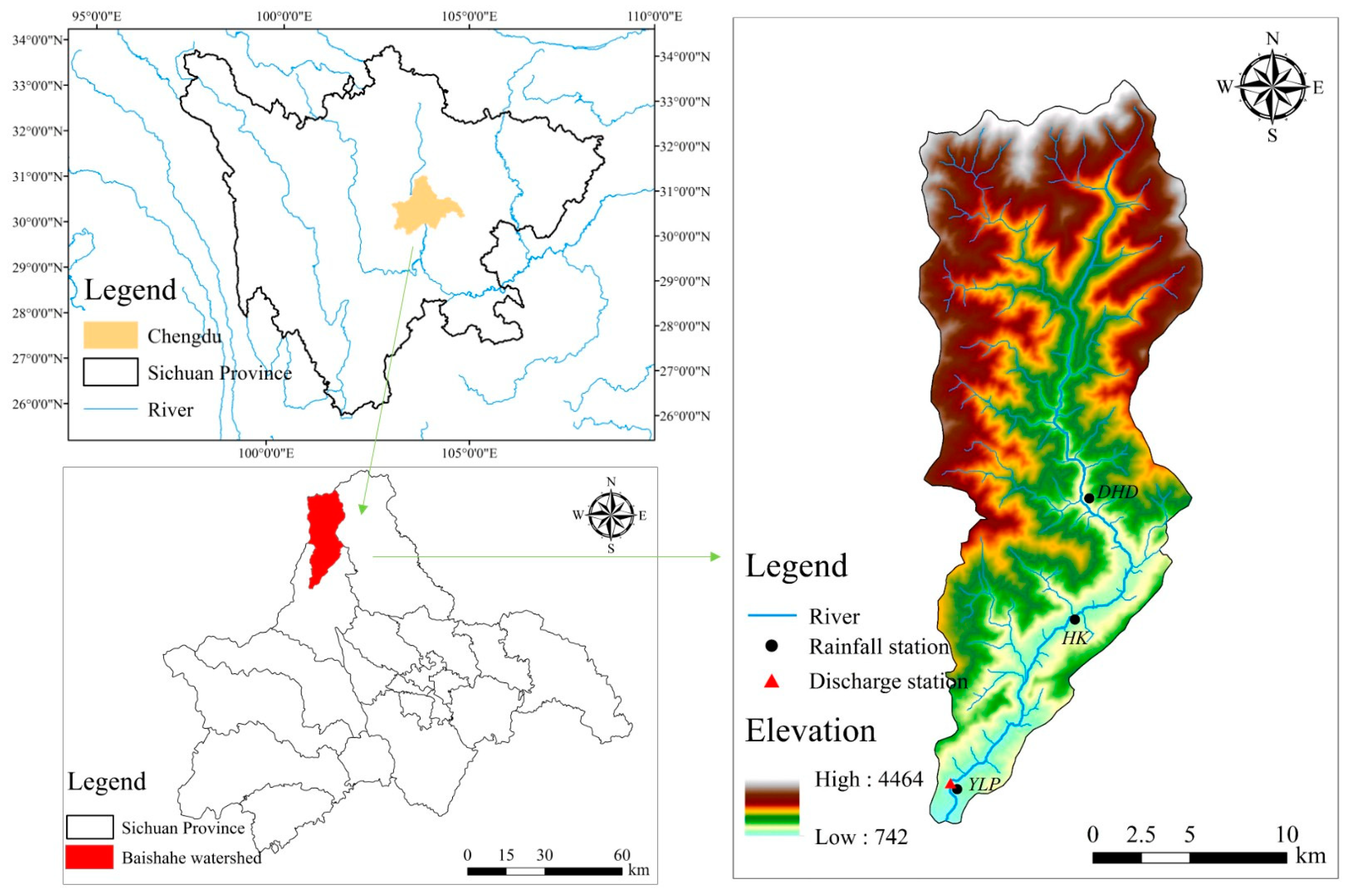
2.1. Study Area

The Baisha River watershed, located in the mountainous area of Sichuan Province, China, was the study area and is shown in Figure 1. The length of the main river stem is approximately 49 km, and the drainage area is 354 km². Because of the complex topographical conditions, the relative height difference is large in the Baisha River watershed, and the meteorological conditions vary significantly in space. The annual average precipitation is approximately 1700 mm, ranging between recorded values of 1400 mm and 2000 mm. The rainfall is unevenly distributed during the year, and more than 60% of the annual precipitation is concentrated in the main flood season from July to September. The river ways in the Baisha River watershed are narrow and deep, with lots of weeds and gravel in the riverbed. Therefore, the Baisha River watershed is prone to flooding in the main flood season, and the runoff formed under the conditions of heavy rainfall, high soil moisture content, and steep channel slope are the characteristics that lead to high peak flood and large flood volume.

2.2. Data Collection

The geospatial data, including digital elevation model (DEM) data with a resolution of 30 m, a land use map, and a soil map, are derived from the Chinese Resource and Environment Data Cloud Platform (http://www.resdc.cn/). A land use map was categorized into five types: agricultural land (0.99%), forest (92.29%), water (1.60%), residential area (0.99%), and bare land (4.12%), as shown in Figure 2a. The soil physical property data (e.g., sand, silt, and clay %) were interpreted from the 1:1,000,000 scale Chinese national soil map, as shown in Figure 2b–d. Hourly precipitation data in the heavy rainfall events during 2010–2015 were collected from three rainfall stations in the Baisha River watershed (see Figure 1), and the discharge time series were collected from discharge stations at the exit of the watershed for calibration and validation. Moreover, through field investigation, a water stage of 756 m at the discharge station was regarded as the critical stage threshold to evacuate people in danger, otherwise it would cause flood damage. In order to determine the early warning index for flash floods (i.e., the rising rate of the flood stage), four 24 h designed rainfall events with different frequencies (1%, 2%, 5%, 10%), which were designed by the rainstorm handbook of Sichuan Province [25], were run in the HEC-HMS model to study the variation in the stage during the flood process.

2.3. The HEC-HMS Hydrological Model

2.3.1. Soil Conservation Service (SCS) Curve Number Method

The method used in the study to calculate total infiltration and runoff generation was the Soil Conservation Service (SCS) curve number (CN) method [26], which uses the following formulas:

$$p_e=\frac{{(p-I_a)}^2}{p-I_a+S},$$

(1)

$$I_a=0.2S,\mathrm{and}$$

(2)

$$S=\frac{25400-254CN}{CN},$$

(3)

where P_e is the accumulated precipitation excess at time t, P is the accumulated rainfall depth at time t, $I_a$ is the initial abstraction, and S is the potential maximum retention.

The parameter CN in the method, which is determined by the hydrologic conditions, land use, soil type, and antecedent moisture [27], can be estimated by the National Engineering Handbook [28].

2.3.2. SCS Unit Hydrograph Method

The SCS unit hydrograph method derived from many small agricultural watersheds has good performance for simulating surface runoff [29]. For the ungauged watershed, the lag time of the SCS unit hydrograph is related to the concentration time as follows:

$$t_{lag}=0.6t_c,$$

(4)

where t_lag is the lag time parameter and t_c is the concentration time.

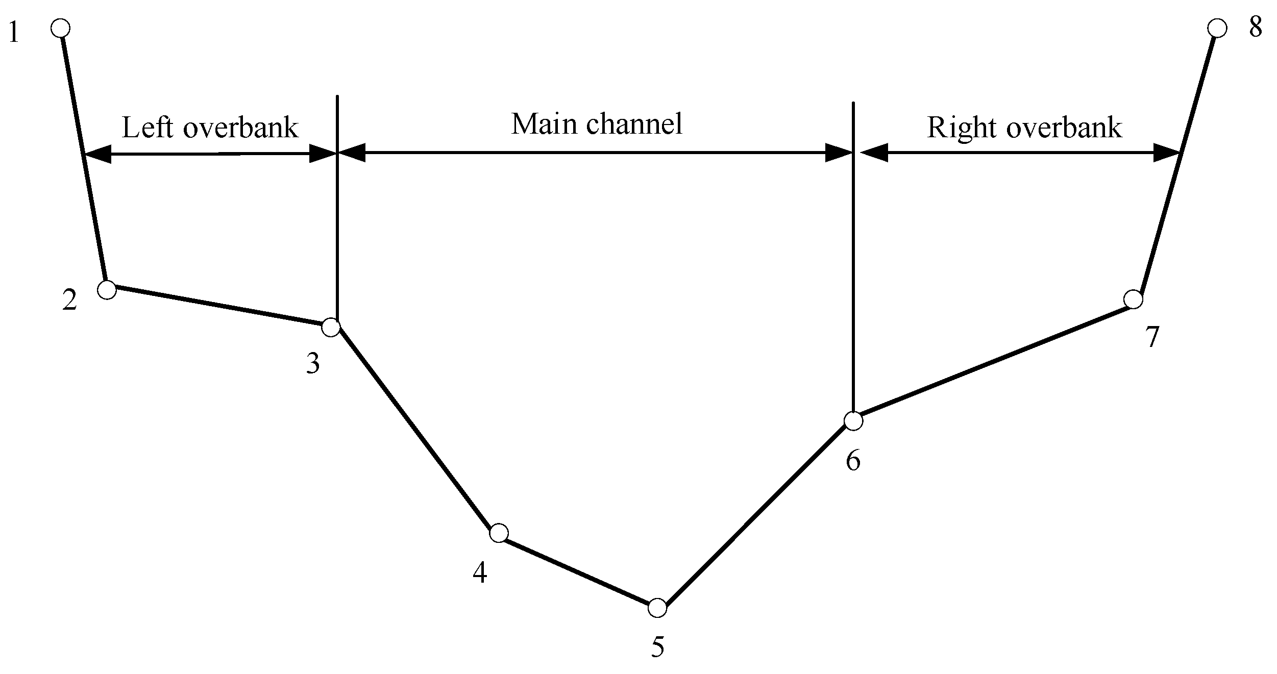
2.3.3. Muskingum–Cunge Method

The Muskingum–Cunge method was used to simulate river routing because the assumptions of this method correspond well to natural channels. The parameters X and K are calculated with the following formulas [30,31]:

$$K=\frac{\Delta x}{c}$$

(5)

$$X=\frac{1}{2}(1-\frac{Q}{B{S}_{0}c\Delta x}),$$

(6)

where $\Delta x$ is the length of the reach, c is the flood velocity, Q is the flood flow, B is the top width of the flood area, and S₀ is the slope of the riverbed.

By using eight pairs of x, y (distance, elevation) values, the 8-point cross-section configuration in the Muskingum–Cunge method was used to describe the cross section of the routing reach. These values are defined specifically, as shown in Figure 3.

The detailed parameters descriptions of the three-step process introduced in the HEC-HMS model are listed in

Table 1. HEC-HMS model components, methods and parameters. SCS: Soil Conservation Service; CN: curve number.

Hydrological Model Component	Method	Parameters	Parameter Estimation Process
Loss	SCS curve number	CN	Calibration
Transform	SCS unit hydrograph	Lag time tlag	Calibration
Routing	Muskingum–Cunge	Cross section	Based on the channel characteristics’
		Manning’s n	calibration

.

2.4. The Inverse Distance Weighting (IDW) Method

The inverse distance weighting (IDW) method [32,33,34] was adopted to calculate the weights of three rain gauges in each sub-watershed in the study area. The general formulas are

$$w_g=\frac{d_g{}^{-b}}{{\displaystyle \sum _{g=1}^G{d}_g{}^{-b}}}\mathrm{and}$$

(7)

$${\widehat{p}}_s=\frac{1}{D}{\displaystyle \sum _{g=1}^G{d}_g{}^{-b}}{p}_g,$$

(8)

where d_g is the distance between the prediction point s and the rain gauge g, G is the number of rain gauges, w_g is the corresponding weight of each gauge, Pg is the value measured at gauge g, and ${\widehat{p}}_s$ is the predicted value at s.

2.5. The Evaluation Criteria of Model Performance

Three criteria were selected to evaluate the simulation performance of the HEC-HMS model, i.e., the relative error of peak flow, the time difference in peak flow occurrence, and the Nash–Sutcliffe (NS) efficiency. The relative error of peak flow and the time difference in peak flow occurrence are widely adopted as the evaluation criteria of flood simulation [5,18,21]. The NS efficiency is one of the most commonly used indicators to reflect the overall fit of hydrographs [35,36]. The detailed formulas are given in

Table 2. The evaluation criteria of model performance. NS: Nash–Sutcliffe.

The Evaluation Criteria	Formulas	Descriptions
The relative error of peak flow	$\frac{Q_{S,P}-Q_{O,P}}{Q_{O,P}}\times 100\%$	$Q_{S,P}$ and $Q_{O,P}$ are the simulated and observed peak flow values, respectively
The time difference in peak flow occurrence	$T_{S,P}-T_{O,P}$	$T_{S,P}$ and $T_{O,P}$ are the simulated and observed time to peak flow values, respectively
NS efficiency	$1-\frac{{\displaystyle {\sum }_{i=1}^N{\left(Q_{S,i}-Q_{O,i}\right)}^2}}{{\displaystyle {\sum }_{i=1}^N{\left(Q_{O,i}-\overline{Q_O}\right)}^2}}$	$Q_{S,i}$ and $Q_{O,i}$ are the simulated and observed discharge values at i time, respectively, $\overline{Q_O}$ is the mean observed discharge value, N is the number of data points

.

3. Results

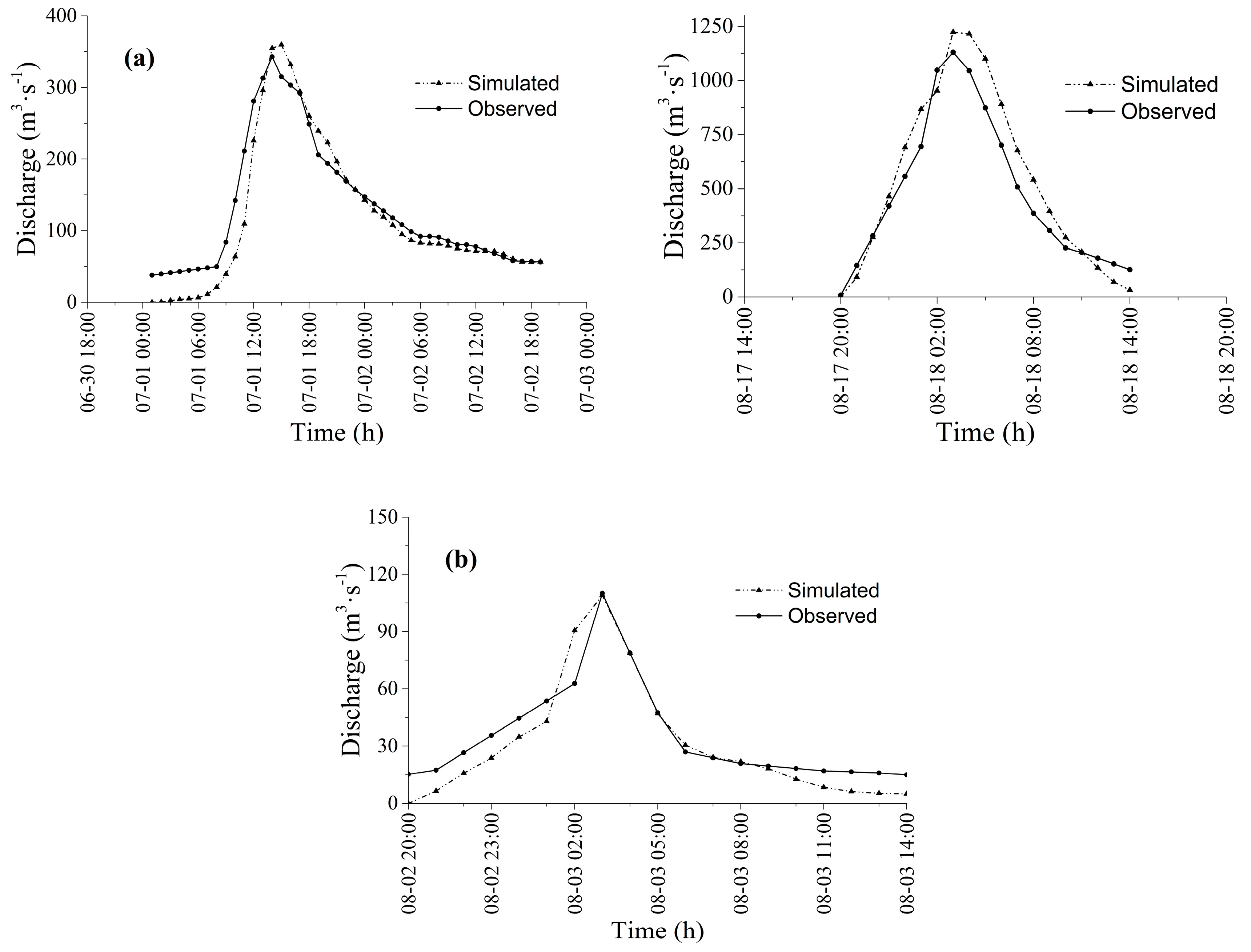
3.1. HEC-HMS Model Calibration and Validation

3.1.1. Model Setup

The Baisha River watershed was divided into 15 sub-watersheds based on DEM data and river network shape by using the HEC-GeoHMS extension tool in ArcGIS (Figure 4). Detailed characteristics for each sub-watershed and channel are shown in

Table 3. Statistical description of the 15 sub-watersheds and main river branches.

Sub-Watershed	Area (km2)	Impervious (%)	Main River Branch	Length (m)	Slope (%)
W670	60.63	0.00	R230	3725.00	3.70
W680	67.44	0.00	R260	2724.40	1.84
W690	26.20	0.00	R270	332.17	1.84
W750	11.04	0.00	R290	2819.60	3.55
W760	15.14	0.00	R310	912.84	5.81
W770	15.93	0.00	R350	1686.80	4.74
W810	21.84	0.02	R370	5085.00	2.40
W850	25.31	0.03	R420	4706.90	1.38
W860	13.57	1.40	R460	4786.90	0.50
W870	8.66	3.36	R470	152.48	0.50
W880	12.47	0.19	R490	8338.30	0.50
W890	14.42	7.06
W910	31.51	0.88
W920	10.25	8.37
W980	20.03	4.13

, and the land use of each sub-watershed are listed in

Table 4. The weights of three rainfall stations and the proportion of land use for each sub-watershed.

Sub-Watershed	DHD	HK	YLP	Agricultural Land	Forest	Water	Residential Area	Bare Land
W670	0.57	0.29	0.14	0.00	0.91	0.02	0.00	0.07
W680	0.57	0.28	0.15	0.00	0.90	0.02	0.00	0.08
W690	0.66	0.24	0.09	0.00	0.96	0.02	0.00	0.02
W750	0.72	0.2	0.07	0.00	0.96	0.02	0.00	0.02
W760	0.67	0.23	0.09	0.00	0.96	0.01	0.00	0.02
W770	0.69	0.23	0.08	0.00	0.96	0.00	0.00	0.04
W810	0.9	0.08	0.02	0.00	0.94	0.01	0.00	0.04
W850	0.76	0.19	0.05	0.01	0.96	0.00	0.00	0.03
W860	0.89	0.1	0.01	0.03	0.93	0.02	0.01	0.01
W870	0.74	0.23	0.04	0.01	0.93	0.01	0.03	0.02
W880	0.39	0.57	0.04	0.00	0.97	0.01	0.00	0.02
W890	0.13	0.84	0.03	0.07	0.82	0.03	0.07	0.00
W910	0.2	0.62	0.18	0.01	0.96	0.01	0.01	0.01
W920	0.04	0.93	0.03	0.11	0.78	0.02	0.08	0.00
W980	0.05	0.18	0.76	0.02	0.89	0.02	0.04	0.03

.

The spatially varied rainfall of each sub-watershed was calculated by the inverse distance method based on the hourly rainfall data of the three meteorological stations. The three meteorological stations are located inside the Baisha River watershed, as shown in Figure 1. The areal weights of the three rain-gauges for each sub-watershed are listed in Table 4.

3.1.2. Model Calibration and Validation

Five independent heavy rainfall events that occurred during 2010–2012 were selected to calibrate the parameters of the HEC-HMS model. Three typical floods that occurred during 2013–2015 were then selected to validate the simulation results, as shown in

Table 5. The results of the flood simulation.

State	Date	Peak Flow (m3·s−1)			The Time Difference in Peak Flow Occurrence (h)	NS Efficiency
		Simulated	Observed	Relative Error (%)
Calibration	14 August 2010	213.20	213.00	0.09	2	0.918
	01 July 2011	359.60	343.00	4.84	1	0.894
	21 August 2011	569.40	535.30	6.37	0	0.845
	27 July 2012	181.30	187.00	−3.05	0	0.852
	18 August 2012	1224.00	1130.00	8.32	0	0.878
Validation	08 July 2013	680.70	750.50	−9.30	0	0.692
	09 July 2014	384.40	414.00	−7.15	0	0.951
	02 August 2015	109.00	110.00	−0.91	0	0.835

. The calibrated parameters of each sub-watershed and channel are shown in

Table 6. Calibrated parameter values.

Sub-Watershed	CN		tlag (min)	Main River Branch	n
	Initial Value	Calibrated Value
W670	70	61	48	R230	0.008
W680	74	64	23	R260	0.008
W690	56	49	69	R270	0.008
W750	74	64	150	R290	0.008
W760	55	48	67	R310	0.008
W770	76	66	19	R350	0.008
W810	55	48	79	R370	0.008
W850	55	48	97	R420	0.008
W860	74	64	44	R460	0.008
W870	58	50	74	R470	0.008
W880	74	65	55	R490	0.008
W890	73	63	65
W910	73	64	97
W920	77	67	8
W980	76	66	97

. Three typically observed and simulated flood processes used during the calibration and validation processes are shown in Figure 5.

The NS efficiency values were between 0.692 and 0.951 with an average value of 0.858, the peak flow relative error was less than 10% and the time difference in the peak flow occurrence was less than 2 h. As shown in Figure 5, the simulated flood process is basically consistent with the observed flood process. The above simulation results of the eight heavy rainfall events show that the HEC-HMS model is effective for simulating the flood process of the Baisha River watershed.

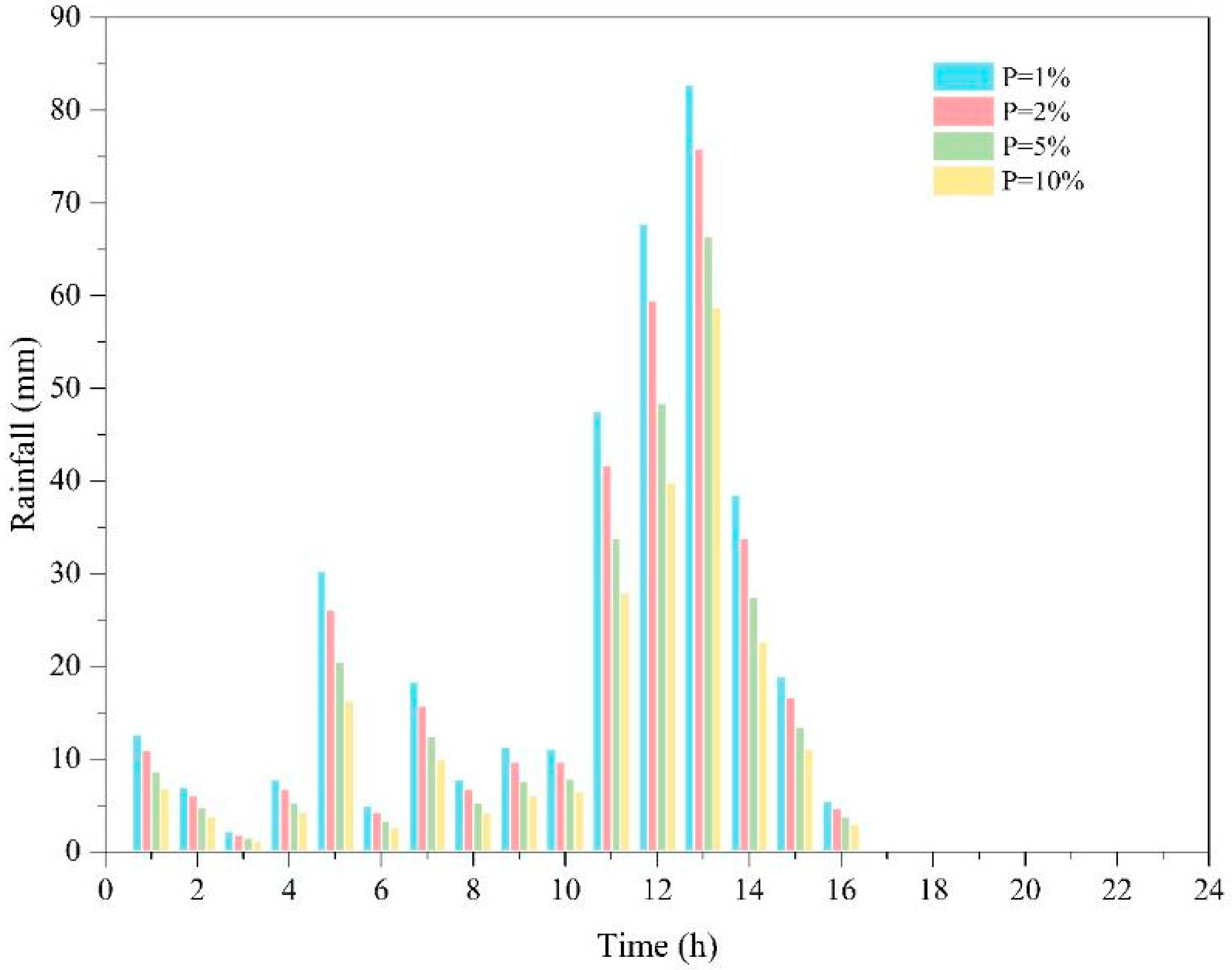
3.2. Design Rainfall with Different Frequencies

The Pearson type III distribution, which is widely used in China, was selected for frequency analysis of the annual maximum 24 h rainfall [22,37,38], and the values of the statistical parameters under different frequencies (p = 1%, 2%, 5%, and 10%) were provided by the Hydrology Handbook of Sichuan Province, as shown in

Table 7. Designed rainfall with different frequencies.

Duration (h)	Statistical Parameters			Designed Rainfall with Different Frequencies (mm)
	Average (mm)	CV	CS/CV	10%	5%	2%	1%
1	40	0.35	3	58.77	66.40	75.89	82.77
6	100	0.5	3	166.67	197.54	237.16	266.52
24	130	0.55	3	224.84	270.67	330.01	374.27

. The distribution of the designed rainfall in time is suggested by the Hydrology Handbook of Sichuan Province, as shown in

Table 8. The distribution of designed rainfall in 24 h.

Duration (h)	P24 h–P12 h (%)	P12 h–P6 h (%)	P1 h (%)
1	11.80
2	6.50
3	2.00
4	7.20
5	28.10
6	4.60
7	17.00
8	7.20
9	10.50
10		6.02
11		25.83
12		36.89
13			100.00
14		20.97
15		10.29
16	5.10
17	0.00
18	0.00
19	0.00
20	0.00
21	0.00
22	0.00
23	0.00
24	0.00

. The hyetograph of the designed rainfall for different frequencies in 24 h is shown in Figure 6.

As shown in Figure 6, heavy rainfall mainly occurs between 11 and 14 h and reaches the highest rainstorm warning signal issued by the China Meteorological Administration; that is, rainfall exceeds 100 mm within 3 h. The maximum precipitation intensity for different frequencies of the designed rainfall occurs at 13 h: 58.77 mm/h (P = 10%), 66.40 mm/h (P = 5%), 75.89 mm/h (P = 2%), and 82.77 mm/h (P = 1%).

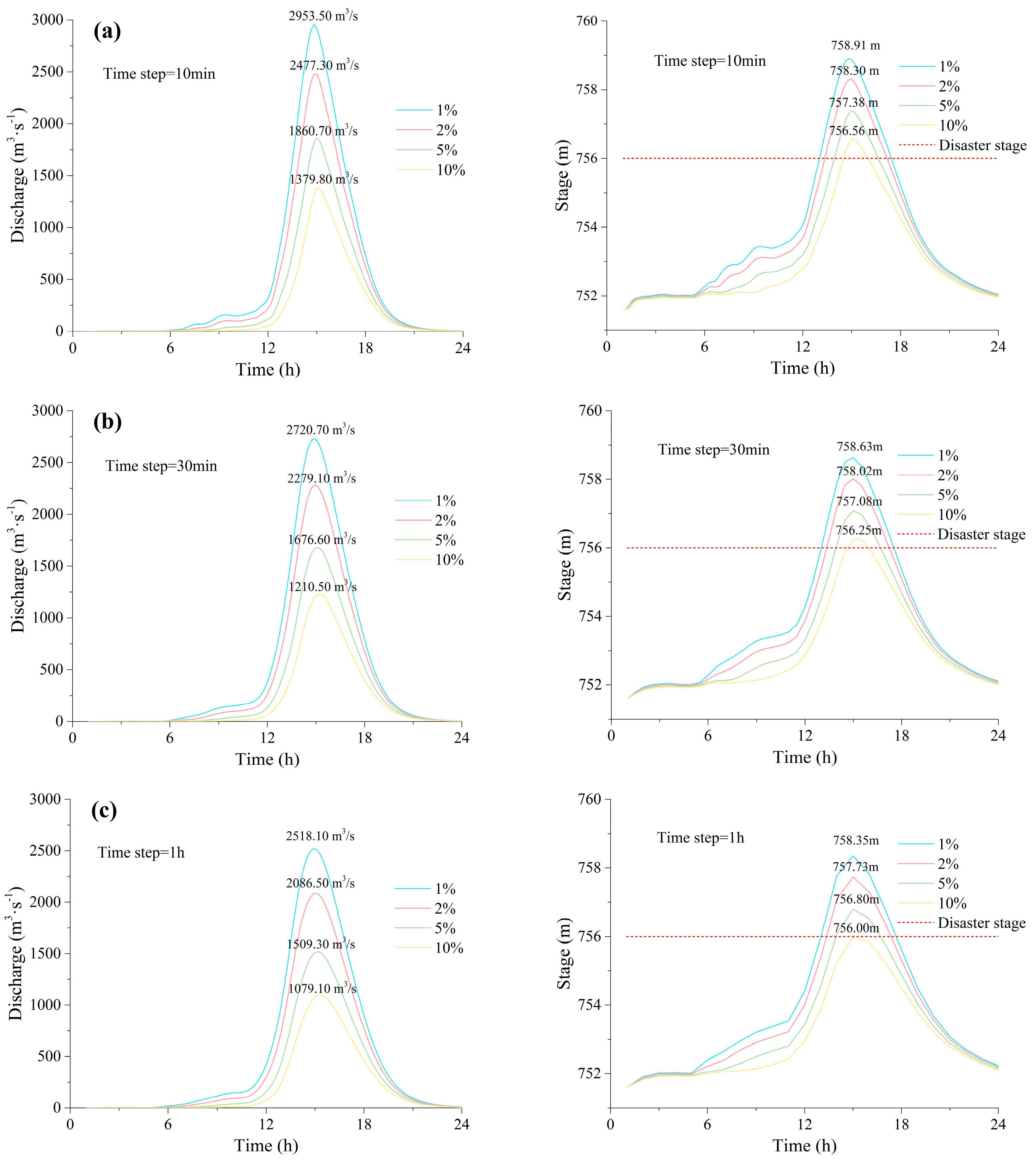
3.3. Simulation Results of Flood Hydrographs

According to the distributions of the four designed 24 h rainfall events, the flood hydrographs with different frequencies were calculated by the HEC-HMS model. Three computation time steps (10 min, 30 min, and 1 h) were used for the simulation to analyze the variation in the flood hydrographs more accurately, and the results are shown in Figure 7.

The results are shown with a similar shape in terms of discharge and stage for different time steps; the 10 min time step produces 10.20% and 21.40% higher discharge with different frequencies of rainfall than those of the 30 min time step and 1 h time step results, respectively.

As the computation time step was reduced, the flood hydrographs became more reasonable, which was conducive to analyzing the variation in the flood stage during the rising flood period. With the hourly data of the designed rainfall events interpolated to shorter computation time steps, the flood hydrographs exhibited a more sensitive response to rainfall, where the flood peak flow was larger, and the flood stage was higher. At 0–5 h, rainfall is lost by infiltration and vegetation interception, and almost no surface runoff occurs. With the soil gradually saturated, surface runoff begins to occur, and the stage rises slowly in 6–10 h. Due to heavy rainfall, the stage rises rapidly within 11–15 h until the peak of the flood hydrographs is reached. In the recession limb of the flood hydrographs, the stage gradually drops below the disaster stage (the critical stage threshold 756 m) after 15 h. The peak of the flood stages with different frequencies, which are shown in Figure 8, exceeds the disaster stage in the Baisha River watershed, and it is necessary to issue early warning signals in time to evacuate people in danger.

4. Discussion

Based on four flood hydrographs with different frequencies, the rising rate of the flood stage was calculated, and the results under three computation time steps are shown in Figure 8.

The variation in the rising rate of the flood stage is more significant as the calculation time step is reduced from 1 h to 10 min. At 0–5 h, due to the relatively large rainfall at the time of 1 h (see Figure 6) and the low initial stage, there is a significant increase in the flood stage at time 1 h, and then the rising rate of the flood stage is almost 0. The rising rate of the flood stage fluctuates (with a rate of 0–1 m/h) together with rainfall during the period of 6–10 h, resulting in the flood stage continuing and rising slowly. During the heavy rainfall period in 11–15 h, the rising rate of the flood stage increases rapidly, exceeding 1 m/h. After 15 h, the flood stage begins to fall as the rising rate of the flood stage is less than 0. The average rising rates in the rising limb of the flood hydrographs increased in multiples from 0–5 h, 6–10 h, and 11–15 h, as shown in Figure 8d. The significant difference in the rising rate of the flood stage during the flood process can be used to identify flood early warning indicators and allow time to evacuate people in dangerous areas.

The three critical times for flood early warning used in the study are marked in Figure 9. The analysis of the flood stage was made with our patented flash flood warning (Xiekang Wang et al., Patent application No. 2019101605606, Patent application publication No. 98 CN109961613A, http://epub.sipo.gov.cn/fullTran.action). During time 0–T1, the flood stage is at a slow rising rate (less than 0.5 m/h), and the flood stage does not reach the disaster stage. The flood stage is in the risk identification period of the flood early warning system, and people in the dangerous area should be ready for evacuation. At the time of T3, the stage reaches the disaster stage. However, that is not an ideal time to issue the flood warning signal, since it is already too late to evacuate the people to safe locations under actual conditions, so the loss caused by floods is difficult to avoid. In order to increase the lead time to mitigate flood loss, T2 was determined as the time to issue an evacuation warning based on the rising rate of the flood stage. During the rapid rise of the rising limb in the flood hydrographs, the flood stage after two hours (determined by the characteristics of the flood and the distribution of the population in the Baisha river watershed) is calculated based on the rising rate at a certain point in time within T1–T3. If the flood stage after two hours based on the rising rate exceeds the disaster stage, it is time for immediate evacuation, marked as T2 in Figure 10. The three critical times in the four flood hydrographs with different frequencies were calculated, and the results are shown in

Table 9. Early warning index based on the rising rate of the flood stage.

The Computation Time Step	Designed Rainfall with Different Frequencies	Time to Preparation for Evacuation T1 (h)	Flood Stage for Preparation for Evacuation (m)	Time to Immediate Evacuation T2 (h)	Flood Stage for Immediate Evacuation (m)
10 min	1%	11.33	753.64	12.17	754.26
	2%	11.33	753.32	12.33	754.11
	5%	11.33	752.89	12.50	753.72
	10%	11.33	752.51	12.83	753.34
0.5 h	1%	11.00	753.55	12.00	754.27
	2%	11.00	753.24	12.50	754.54
	5%	11.00	752.82	12.50	753.85
	10%	11.00	752.44	13.00	753.83
1 h	1%	11.00	753.54	12.00	754.40
	2%	11.00	753.23	13.00	755.39
	5%	11.00	752.80	13.00	754.55
	10%	11.00	752.43	14.00	755.25
The Computation Time Step	Design Rainfall Events with Different Frequencies	Rising Rate of Flood Stage at T2 (m·h−1)	Time to Disaster Stage T3 (h)	Disaster Stage (m)	Advance Time for Issuing Early Warning Signal (h)
10 min	1%	1.28	13.03	756.00	0.86
	2%	1.51	13.35		1.02
	5%	1.51	13.94		1.44
	10%	1.23	14.51		1.68
0.5 h	1%	1.02	13.01		1.01
	2%	1.34	13.29		0.79
	5%	1.06	13.82		1.32
	10%	1.07	14.51		1.51
1 h	1%	0.86	13.01		1.01
	2%	1.38	13.36		0.36
	5%	1.12	13.94		0.94
	10%	1.37	15.00		1.00

.

Table 9 shows that the time to immediate evacuation T2 and the time to the disaster stage T3 lag as the frequency of the design rainfall event declines. Under three computation time steps, the flood stage for immediate evacuation, which is the corresponding stage at time T2, varies from 753.83 to 755.39 m for different designed rainfall events. The stage of preparation for evacuation that corresponds to the flood stage at T1 ranges from 752.43 to 753.64 m for different designed rainfall events. Most of the rising rates of the flood stage at the time for immediate evacuation T2 exceed 1 m/h. If the warning information is not released in time, the flood stage reaches the disaster stage in a short time. The advanced time for issuing the early warning signal is the difference between T2 and T3, which is generally greater than 1 h.

The average early warning indicators under the three computation time steps was calculated to determine the early warning indicators in the Baisha River watershed, as shown in Figure 10. The flood stage for immediate evacuation is between 754.04 and 754.68 m with an average value of 754.29 m. For conservative considerations, 754.04 m is the critical early warning index in the flood stage for evacuating people to safe locations. Another critical early warning indicator is the rising rate of the flood stage at the time for immediate evacuation T2, which varies from 1.05 to 1.41 m/h, and the average value is 1.23 m/h. When the stage is at 754.04 m and the rising rate exceeds 1.05 m/h, flood damage is very likely to occur in the Baisha River watershed within two hours. According to the critical early warning index in the flood stage and the rising rate, the time of issuing the early warning signal is between 0.72 and 1.40 h for designed rainfall events with different frequencies. The flood stage and the rising rate of the flood stage, as early warning indicators, can effectively increase the lead time for evacuation compared to the flood stage alone.

5. Conclusions

In this study, flood hydrographs under designed rainfall events with different frequencies for the study area were obtained using the HEC-HMS model. Based on the variation in the rising rate of the flood stage in the rising limb of the flood hydrographs, the early warning indicators for the advanced time to issue warning signals were established. The conclusions of this study are as follows:

(1)

By using the HEC-GeoHMS extension tool in ArcGIS, the characteristic information (e.g., land use, soil type, and slope) was extracted to determine the parameters for the HEC-HMS model. The results of the model calibration and validation demonstrated that the HEC-HMS model was effective for the simulation of mountain floods in the study area. The application of the HEC-HMS model to flash flood early warning should be encouraged in other watersheds in China, especially in small watersheds that lack sufficient hydrological data.

(2)

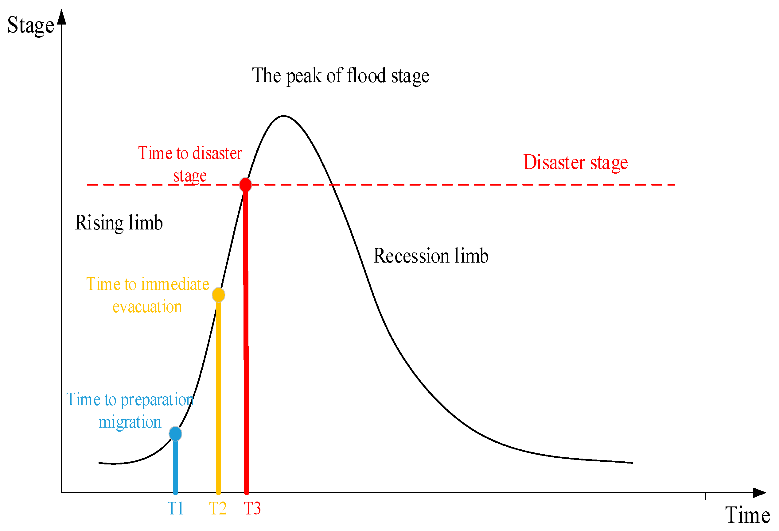
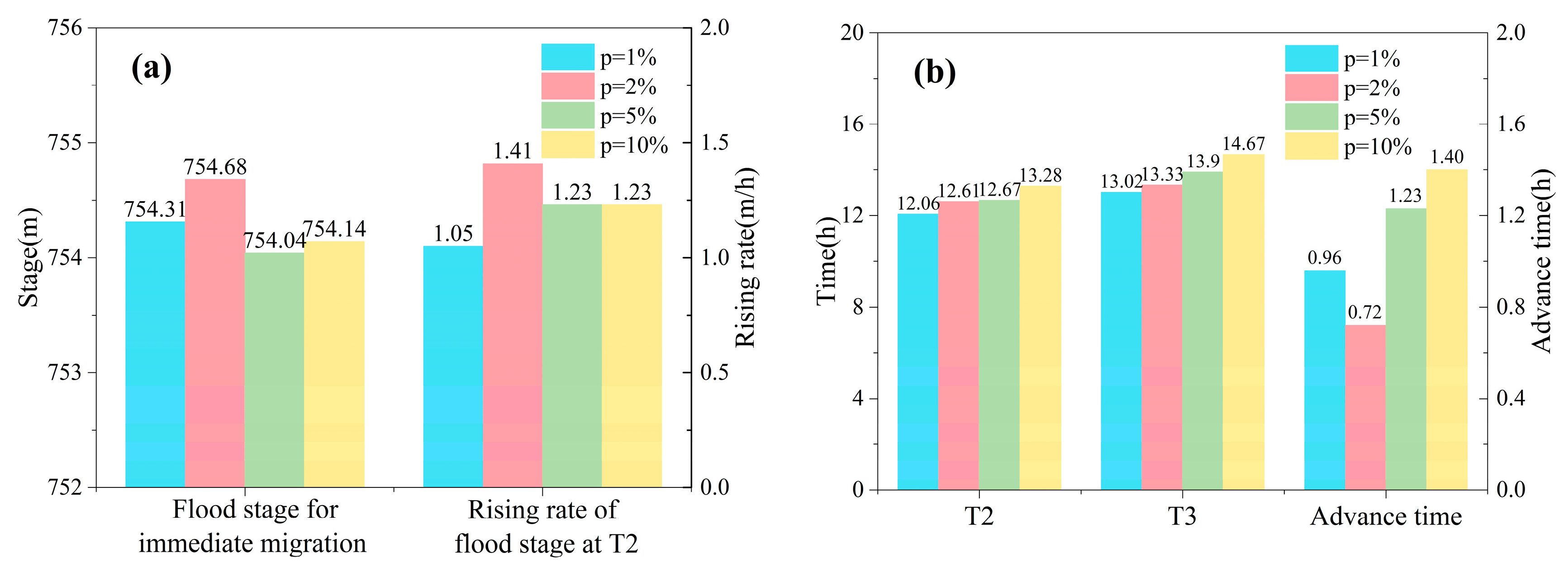
According to the analysis of flood hydrographs with different frequencies, the rising rates of the flood stage in the rising limb of the flood hydrographs are substantially different, and can be divided into three parts (0–5 h, 6–10 h, 11–15 h). The rising rate of flood stage increases in multiples in the three parts of the flood hydrographs. In addition, the variation in the flood stage has a more sensitive response to rainfall when the computation time step decreases.

(3)

The two critical early warning indicators, which are the flood stage for immediate evacuation (754.04 m) and the rising rate (1.05 m/h), were determined based on the variation in the flood stage. Therefore, flash flood early warning in mountainous areas is no longer limited to the signal index (e.g., rainfall, flow or flood stage), and the advanced time determined by the rising rate before it reaches the warning flood stage can be applied in emergency management.

Due to the scarcity and incompleteness of hydrologic data in mountainous watersheds, it is difficult to analyze the impact of rainfall uncertainty on critical early warning indicators. Future research in this watershed should be supplemented with relevant data from field measurements, and more influencing factors (e.g., rainfall spatiotemporal resolution, rainfall intensity, and different rainfall patterns) should be taken into account to determine more accurate critical thresholds for flood early warning.

References

1. Hall, J.; Arheimer, B.; Borga, M.; Brázdil, R.; Claps, P.; Kiss, A.; Kjeldsen, T.R.; Kriaučiūnienė, J.; Kundzewicz, Z.W.; Lang, M.; et al. Understanding flood regime changes in Europe: A state-of-the-art assessment. Hydrol. Earth Syst. Sci. 2014, 18, 2735–2772. [Google Scholar] [CrossRef] [Green Version]
2. Kvočka, D.; Falconer, R.A.; Bray, M. Flood hazard assessment for extreme flood events. Nat. Hazards 2016, 84, 1569–1599. [Google Scholar] [CrossRef] [Green Version]
3. Golian, S.; Saghafian, B.; Maknoon, R. Derivation of Probabilistic Thresholds of Spatially Distributed Rainfall for Flood Forecasting. Water Resour. Manag. 2010, 24, 3547–3559. [Google Scholar] [CrossRef]
4. He, B.S.; Huang, X.L.; Guo, L. China’s mountain flood disaster prevention route and core consstuction content. China Flood Drought Manag. 2012, 22, 19–22. [Google Scholar]
5. Zhai, X.; Guo, L.; Liu, R.; Zhang, Y. Rainfall threshold determination for flash flood warning in mountainous catchments with consideration of antecedent soil moisture and rainfall pattern. Nat. Hazards 2018, 94, 605–625. [Google Scholar] [CrossRef]
6. Kang, A.; Zhang, K.; Liang, J.; Yan, B.; Lei, X.; Guo, J. Applying the dynamic critical precipitation method for flash flood early warning. Pol. J. Environ. Stud. 2019, 28, 1727–1733. [Google Scholar] [CrossRef]
7. Jia, P.; Liu, R.; Ma, M.; Liu, Q.; Wang, Y.; Zhai, X.; Xu, S.; Wang, D. Flash flood simulation for ungauged catchments based on the distributed hydrological model. Water 2019, 11, 76. [Google Scholar] [CrossRef] [Green Version]
8. Massazza, G.; Tamagnone, P.; Wilcox, C.; Belcore, E.; Pezzoli, A.; Vischel, T.; Panthou, G.; Ibrahim, M.H.; Tiepolo, M.; Tarchiani, V.; et al. Flood hazard scenarios of the Sirba River (Niger): Evaluation of the hazard thresholds and flooding areas. Water (Switzerland) 2019, 11, 1018. [Google Scholar] [CrossRef] [Green Version]
9. Liu, C.; Guo, L.; Ye, L.; Zhang, S.; Zhao, Y.; Song, T. A review of advances in China’s flash flood early-warning system. Nat. Hazards 2018, 92, 619–634. [Google Scholar] [CrossRef] [Green Version]
10. Hapuarachchi, H.A.P.; Wang, Q.J.; Pagano, T.C. A review of advances in flash flood forecasting. Hydrol. Process. 2011, 25, 2771–2784. [Google Scholar] [CrossRef]
11. Petersen-Øverleir, A.; Reitan, T. Accounting for rating curve imprecision in flood frequency analysis using likelihood-based methods. J. Hydrol. 2009, 366, 89–100. [Google Scholar] [CrossRef]
12. Ashrafi, M.; Chua, L.H.C.; Quek, C.; Qin, X. A fully-online Neuro-Fuzzy model for flow forecasting in basins with limited data. J. Hydrol. 2017, 545, 424–435. [Google Scholar] [CrossRef]
13. Biondi, D.; De Luca, D.L. Performance assessment of a Bayesian Forecasting System (BFS) for real-time flood forecasting. J. Hydrol. 2013, 479, 51–63. [Google Scholar] [CrossRef]
14. Cools, J.; Vanderkimpen, P.; El Afandi, G.; Abdelkhalek, A.; Fockedey, S.; El Sammany, M.; Abdallah, G.; El Bihery, M.; Bauwens, W.; Huygens, M. An early warning system for flash floods in hyper-arid Egypt. Nat. Hazards Earth Syst. Sci. 2012, 12, 443–457. [Google Scholar] [CrossRef]
15. Wałęga, A.; Cupak, A.; Amatya, D.M.; Drożdżal, E. Comparison of Direct Outflow Calculated By Modified Scs-Cn Methods for Mountainous and Highland Catchments in Upper Vistula Basin, Poland and Lowland Catchment in South Carolina, USA. Acta Sci. Pol. Form. Circumiectus 2017, 16, 187–207. [Google Scholar] [CrossRef]
16. Zoccatelli, D.; Borga, M.; Viglione, A.; Chirico, G.B.; Blöschl, G. Spatial moments of catchment rainfall: Rainfall spatial organisation, basin morphology, and flood response. Hydrol. Earth Syst. Sci. 2011, 15, 3767–3783. [Google Scholar] [CrossRef] [Green Version]
17. Abushandi, E.; Merkel, B. Modelling Rainfall Runoff Relations Using HEC-HMS and IHACRES for a Single Rain Event in an Arid Region of Jordan. Water Resour. Manag. 2013, 27, 2391–2409. [Google Scholar] [CrossRef]
18. Joo, J.; Kjeldsen, T.; Kim, H.J.; Lee, H. A comparison of two event-based flood models (ReFH-rainfall runoff model and HEC-HMS) at two Korean catchments, Bukil and Jeungpyeong. KSCE J. Civ. Eng. 2014, 18, 330–343. [Google Scholar] [CrossRef]
19. Caruso, B.S.; Rademaker, M.; Balme, A.; Cochrane, T.A. Flood modelling in a high country mountain catchment, New Zealand: Comparing statistical and deterministic model estimates for ecological flows. Hydrol. Sci. J. 2013, 58, 328–341. [Google Scholar] [CrossRef] [Green Version]
20. Oleyiblo, J.O.; Li, Z.J. Application of HEC-HMS for flood forecasting in Misai and Wan’an catchments in China. Water Sci. Eng. 2010, 3, 14–22. [Google Scholar]
21. Yuan, W.; Liu, M.; Wan, F. Calculation of Critical Rainfall for Small-Watershed Flash Floods Based on the HEC-HMS Hydrological Model. Water Resour. Manag. 2019, 33, 2555–2575. [Google Scholar] [CrossRef]
22. Wang, Q.; Xu, Y.; Wang, J.; Lin, Z.; Dai, X.; Hu, Z. Assessing sub-daily rainstorm variability and its effects on flood processes in the Yangtze River Delta region. Hydrol. Sci. J. 2019, 64, 1–10. [Google Scholar] [CrossRef]
23. Azam, M.; Kim, H.S.; Maeng, S.J. Development of flood alert application in Mushim stream watershed Korea. Int. J. Disaster Risk Reduct. 2017, 21, 11–26. [Google Scholar] [CrossRef] [Green Version]
24. Halwatura, D.; Najim, M.M.M. Application of the HEC-HMS model for runoff simulation in a tropical catchment. Environ. Model. Softw. 2013, 46, 155–162. [Google Scholar] [CrossRef]
25. Sichuan Province Water Resources Department. Rainfall Handbook of Design Storm Flood in Medium and Small River Basins in Sichuan Province; Sichuan Province Water Resources Department: Chengdu, China, 1984. [Google Scholar]
26. Geetha, K.; Mishra, S.K.; Eldho, T.I.; Rastogi, A.K.; Pandey, R.P. SCS-CN-based continuous simulation model for hydrologic forecasting. Water Resour. Manag. 2008, 22, 165–190. [Google Scholar] [CrossRef]
27. Mishra, S.K.; Singh, V.P. Long-term hydrological simulation based on the Soil Conservation Service curve number. Hydrol. Process. 2004, 18, 1291–1313. [Google Scholar] [CrossRef]
28. USDA Section 4: Hydrology. SCS National Engineering Handbook; USDA Soil Conservation Service: Washington, DC, USA, 1972. [Google Scholar]
29. Jin, H.; Liang, R.; Wang, Y.; Tumula, P. Flood-runoff in semi-arid and sub-humid regions, a case study: A simulation of Jianghe watershed in northern China. Water (Switzerland) 2015, 7, 5155–5172. [Google Scholar] [CrossRef] [Green Version]
30. Cunge, J.A. On the subject of a flood propagation computation method (musklngum method). J. Hydraul. Res. 1969, 7, 205–230. [Google Scholar] [CrossRef]
31. Ponce, V.M.; Yevjevich, V. Muskingum-Cunge method with variable Paremeters. J. Hydraul. Div. 1978, 104, 1663–1667. [Google Scholar]
32. Ruelland, D.; Ardoin-Bardin, S.; Billen, G.; Servat, E. Sensitivity of a lumped and semi-distributed hydrological model to several methods of rainfall interpolation on a large basin in West Africa. J. Hydrol. 2008, 361, 96–117. [Google Scholar] [CrossRef]
33. Pingale, S.M.; Khare, D.; Jat, M.K.; Adamowski, J. Spatial and temporal trends of mean and extreme rainfall and temperature for the 33 urban centers of the arid and semi-arid state of Rajasthan, India. Atmos. Res. 2014, 138, 73–90. [Google Scholar] [CrossRef]
34. Xu, W.; Zou, Y.; Zhang, G.; Linderman, M. A comparison among spatial interpolation techniques for daily rainfall data in Sichuan Province, China. Int. J. Climatol. 2015, 35, 2898–2907. [Google Scholar] [CrossRef]
35. Legates, D.R.; McCabe, G.J. Evaluating the use of “goodness-of-fit” measures in hydrologic and hydroclimatic model validation. Water Resour. Res. 1999, 35, 233–241. [Google Scholar] [CrossRef]
36. Jain, S.K.; Sudheer, K.P. Fitting of hydrologic models: A close look at the nash-sutcliffe index. J. Hydrol. Eng. 2008, 13, 981–986. [Google Scholar] [CrossRef]
37. Ministry of Water Resources of the People’s Republic of China. Regulation for Calculating Design Flood of Water Resources and Hydropower Projects; China Water & Power Press: Beijing, China, 2006. [Google Scholar]
38. Li, Z.; Zhang, H.; Singh, V.P.; Yu, R.; Zhang, S. A simple early warning system for flash floods in an ungauged catchment and application in the Loess Plateau, China. Water 2019, 11, 426. [Google Scholar] [CrossRef] [Green Version]
Figure 1. Study area.
Water 12 00255 g001
Figure 2. Land use and soil type in the study area: land use (a), clay (b), sand (c), and silt (d).
Water 12 00255 g002
Figure 3. Eight-point cross-section configuration.
Water 12 00255 g003
Figure 4. Spatial distribution of 15 sub-watersheds and main river branches in the red line.
Water 12 00255 g004
Figure 5. Simulated and observed hydrographs for calibration and validation: (a) calibration of the hydrograph for the floods on 01 July 2011 and 18 August 2012, (b) validation of the hydrograph for the flood on 02 August 2015.
Water 12 00255 g005
Figure 6. Rainfall hyetograph of designed storm for 10, 20, 50, and 100-year return period in 24 h.
Water 12 00255 g006
Figure 7. The simulated results of flood hydrographs with three computation time steps (10 min (a), 30 min (b), and 1 h (c)) based on four frequencies of designed rainfall (1%, 2%, 5%, and 10%).
Water 12 00255 g007
Figure 8. The variation in the rising rate of the flood stage with three computation time steps (10 min (a), 30 min (b), and 1 h (c)), and the average rising rates in the rising limb of the flood hydrographs (d).
Water 12 00255 g008
Figure 9. The three critical times for early flood warning.
Water 12 00255 g009
Figure 10. The average of early warning indicators under different return periods of rainfall: (a) the rising rate and the corresponding flood stage, (b) the advance time for early warning.
Water 12 00255 g010