Sediment Management at Run-of-River Reservoirs Using Numerical Modelling


1
Chair of Hydraulic and Water Resources Engineering, Technical University of Munich, Arcisstrasse 21, D-80333 Munich, Germany
2
Water Authority Rosenheim, Königstrasse 19, D-83022 Rosenheim, Germany
*
Author to whom correspondence should be addressed.
Water 2020, 12(1), 249; https://doi.org/10.3390/w12010249
Submission received: 12 December 2019
/
Revised: 7 January 2020
/
Accepted: 10 January 2020
/
Published: 16 January 2020
(This article belongs to the Section Hydraulics and Hydrodynamics)
Abstract
:The worldwide storage volume of reservoirs is estimated to decrease by 0.5–1% per year due to sedimentation, which is higher than the gain in volume by newly built dams. For water supply or flood protection, the preservation of the storage volume is crucial. Operators and authorities, therefore, need sediment management concepts to ensure that the storage volume is sufficient. In this study, we developed a sediment-flushing concept using 2D numerical modelling for a run-of-river hydropower plant located in the Saalach River in southeastern Germany. The calibrated bed elevation was used as the initial bed for a number of simulations with different discharge regimes under varying operational schemes. By comparing the simulated results, we propose an appropriate flushing scheme in terms of intensity and duration to obtain a balance of sediment regime in the river. Furthermore, we demonstrate that such an optimised sediment management can generate synergies for improving measures of flood protection.
1. Introduction
Water is a limited resource, and efficient and sustainable distribution between different sectors is and will be of high importance worldwide [1]. Engineering structures, e.g., dams or weirs, are built to use water more efficiently or to ensure its availability. These structures store water in reservoirs and thus interrupt the hydromorphodynamic continuity of the river; not only water but also sediment transported by the river is accumulated. Globally, this unintended process has led to a decrease of around 0.5–1% of the available storage volume of water and simultaneously to higher riverbed levels [2]. It is predicted that at this decreasing rate around 1/4 of worldwide dams may be lost in the next 25–50 years [3]. Despite a loss in storage volume, the resulting higher riverbed level has additional negative consequences, such as increased flood risk.
In this paper, we focus on the consequences of sedimentation at a run-of-river hydropower plant (HPP) and the corresponding reservoir in a mountainous region. At such structures, water is dammed up to a certain level of operation to increase the difference in height between upstream and downstream water levels, i.e., the head, and thus the energy production potential [4]. In addition, artificial embankments, or storage levees, are commonly built along the upstream river section to further increase the cross-section area of channels, and thus the possible head and the storage capacity of the reservoir. Sedimentation in run-of-river reservoirs lowers the storage volume of water, which might affect the water availability; however, the increase of the riverbed elevation in the reservoir is much more severe in this case. A higher riverbed causes higher water levels, especially during flood events, and can lead to a breach of the designed embankments [5]. Commonly, during high discharge events, the outlets of the dam or the gates/weirs are opened to stop the water level exceeding a defined threshold, which is lower than the crest of the designed embankments along the river. If the riverbed elevation is too high, this strategy will fail and thus cause harmful inundation. Especially in mountainous regions, where rivers have powerful currents causing high sediment loads of coarse gravel, the correlation between the flow, the morphology and engineering constructions is high. Therefore, measures dealing with sedimentation is a closely studied topic in the literature [4,6].
Developments in achieving a more sustainable sediment management strategy are of high interest for HPP owners, environmental agencies and local residents alike. Depending on the river characteristics (i.e., bed grain size distribution, slope and discharge) and the characteristics of the technical structure (i.e., geometry, length, height and width) different measures and management strategies are appropriate. Annandale et al. [4] classified them into four groups: Reduction of sediment supply from upstream sections, routing of sediment through the dam, removal sediment deposits in the reservoir and adaptive strategies. Numerical and/or physical modelling of reservoirs are important tools for engineers in developing such strategies. Integrative, coupled numerical hydromorphological models are particularly suitable as they can represent reality accurately and are more flexible than physical models. One-dimensional (1D) numerical models are the standard application since they have low computational requirements and deliver solutions quickly, but they include several simplifications and limitations. However, they are applied in several studies [7,8,9]. More advanced two-dimensional (2D) or three-dimensional (3D) models are more accurate, and thus able to represent reality in more detail, but they require higher computational resources and more data, which are not commonly available. However, several of these numerical models are used to study sedimentation at reservoirs. Gallerano and Cannata [10] proposed a 3D model, which is calibrated on suspended sediment concentration measurements, and assessed the impact of flushing on downstream reaches. Ateeq-Ur-Rehman [11] used a 2D depth-averaged model to predict sedimentation at the Indus River in Pakistan, on a large spatial and temporal scale. Further, Chaudahary et al. [12] showed that numerical 1D in general, and 2D models for detailed analyses are suited to investigating sediment-flushing operations. Bui and Rutschmann [13] demonstrated that a 2D model, which includes treatment for secondary flows, would be suited to simulating sediment processes in complex geometries.
Methods of mechanical excavation or flushing of sediment are commonly applied in run-of-river reservoirs to counter sedimentation. While mechanical excavation is very expensive and time-consuming, flushing can be more effective and efficient, as it uses the power of the river [4,14]. Drawdown flushing is performed by lowering the water levels in the whole reservoir, leading to free-flowing (i.e., riverine flow) conditions at the dam [15]. The accelerated flow causes high shear stresses on the riverbed, and thus high sediment transport rates, resulting finally in a lower riverbed. However, the complexity of the morphological processes and natural variability, which makes each hydrological year unique, requires adaptive solutions and knowledge of flushing schemes.
This paper proposes a concept for developing a sediment management strategy based on drawdown flushing operations using 2D hydromorphological numerical modelling. The framework was applied to an existing HPP in the Saalach River, in southeastern Germany. Two study objectives were considered: (1) evaluate the potential of reservoir flushing to re-establish the sediment continuity in the river by different weir operating regulations; and (2) apply the model with the proposed flushing schemes to a longer and consecutive period.
2. Methods
2.1. Study Area and Data Description
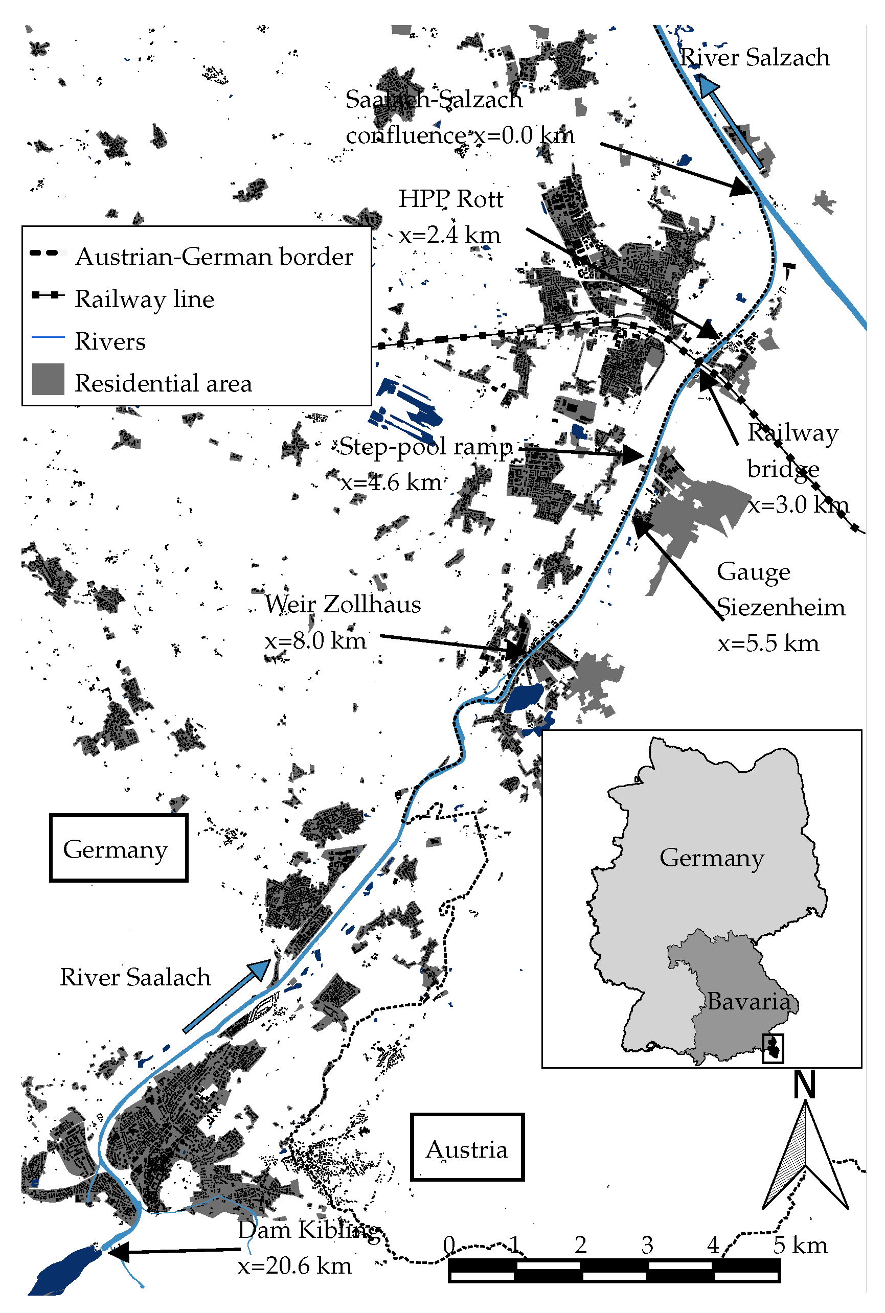
The present study follows the work of Reisenbüchler et al. [5] and Reisenbüchler et al. [16], who developed a numerical hydromorphological model of a section of the Saalach River from upstream at x = 8.0 km, below an unregulated weir, to the HPP at x = 2.4 km downstream, as shown in Figure 1. The water surface and bed elevation used in this study were therefore referenced to the German vertical elevation system in metres above sea level (masl). This hydromorphological numerical model was successfully calibrated and validated for a period of eight years. More details on the model development can be found in [5,16].
The riverbed consists of coarse gravels with an arithmetic mean diameter of and a maximum diameter of = 140 mm. The high bed slope (up to 0.047) and high possible discharge generate high hydraulic forces, and thus a high potential of sediment transport. Due to the engineering works at the Kibling HPP-Dam (at x = 20.6 km) near the city of Bad Reichenhall, the sediment regime is unbalanced in this region, requiring sediment management strategies [16,17]. Weiss [17] reported an average 95,000 m3/year of sediment deposits in the reservoir. Reducing the amount of sediment available downstream can lead to increased erosion of the bed and banks. This may turn depositional areas into erosional ones or increase the rate of erosion where it already exists. For the dynamic stabilisation of the downstream river reach, an artificial sediment supply station has been established. The dimension of the amount of material and its grain-size composition is mainly aimed at stabilising the transport capacity of the reach and the grain-size of the natural bed load there. Since 1999, on average 50,000 m3/year of sediment were supplied to the river. In the future, this amount will be reduced to approximately 30,000 m3/year, since investigations have shown that a lower amount is enough to keep the riverbed stable in free-flowing sections [16]. At the gauging station x = 5.5 km, discharge and water level are measured, which serves as the inflow boundary condition of the numerical model. Analysing the discharge data for 1976–2015 yields the following statistical flow data [18]: mean discharge , mean flood discharge and 100-year return period flood discharge . Furthermore, Reisenbüchler et al. [16] provided a sediment-rating-curve (SRC) at the model inlet, which describes the amount of transported sediment corresponding to the discharge of water and the annually supplied material at the Kibling dam.
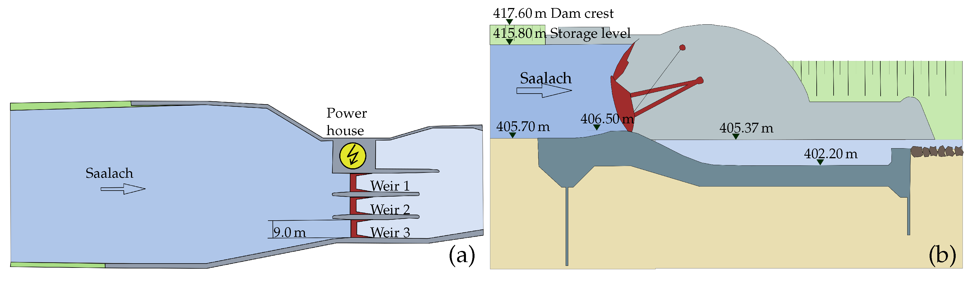
Moreover, at the HPP Rott (x = 2.4 km), which is the model outlet, there is a legally binding operational ordinance for the water level in the reservoir. This document defines how the reservoir is to be operated depending on the discharge in the river. In addition, we obtained the water level measurements in the reservoir from 2005 and 2013, indicating sediment-flushing performed. The HPP has three structurally identical weirs sections, which allows a variable regulation of the water surface elevation. Figure 2 shows the most important facilities of the HPP schematically from the top view (Figure 2a), and as a longitudinal section through one weir (Figure 2b), which are considered in this study.
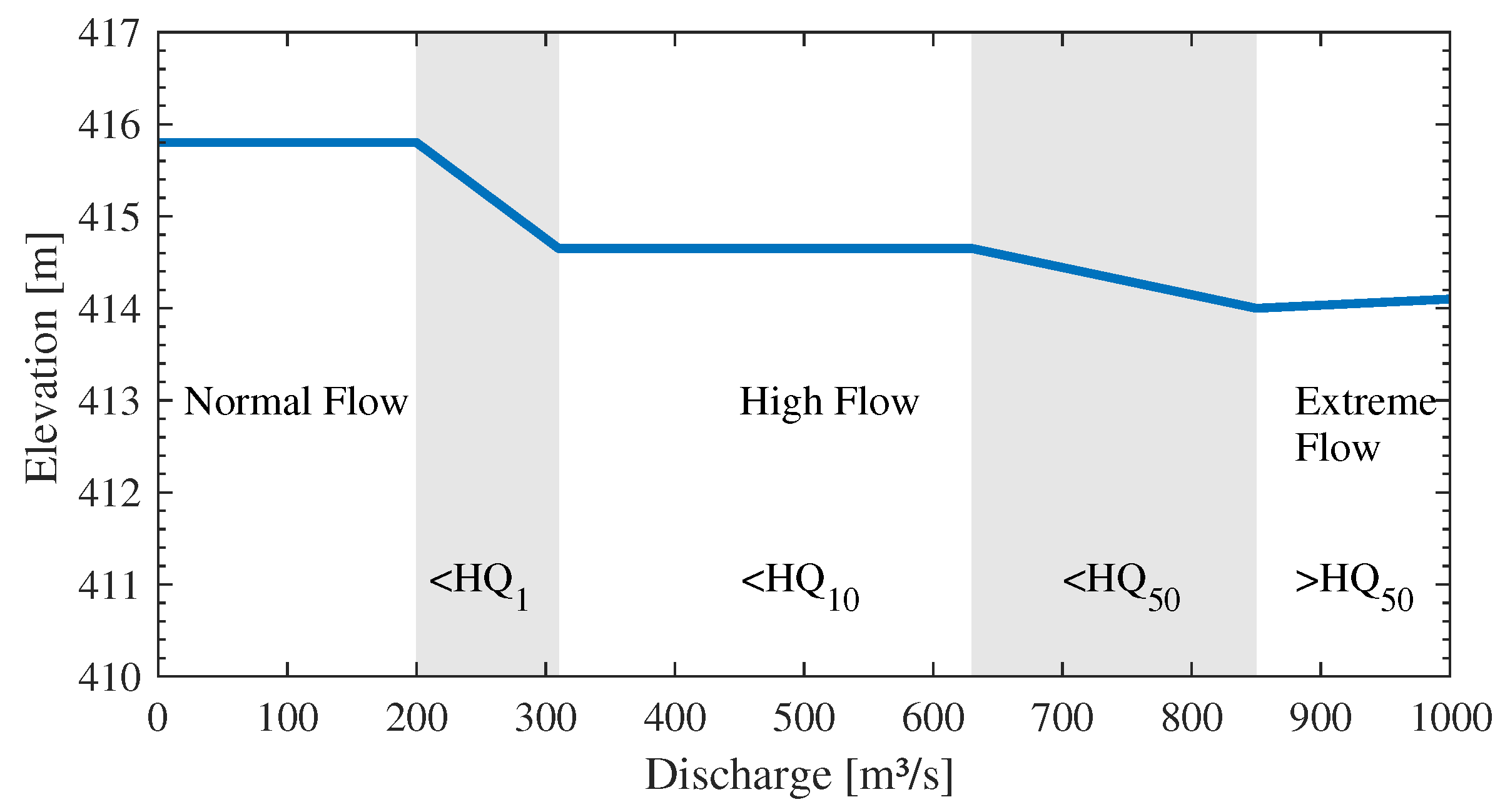
We modelled the official weir ordinance by applying a stage-discharge relation (see Figure 3). The possible range of discharges is classified into three operational modes: normal, high and extreme flow. For discharges lower than , the water level can be up to the maximum storage level of Zf,S = 415.80 m. When the discharge exceeds , the water level has to be decreased to Zf = 414.65 m by opening the weirs, considering a maximum speed of . This speed must not be exceeded; otherwise, the stability of the embankments is endangered [19]. If the discharge exceeds , the water level must be further lowered to Zf = 414.00 m, taking into account the same lowering speed. In the case of extreme floods and discharges higher than , the weirs are completely open, allowing free-flowing conditions. A rating-curve for the free-flowing condition at the HPP is approximated with a potential function Zf = 403.33Q0.0034. The three weirs have a total capacity to allow the design flood discharge to pass harmlessly.
2.2. Numerical Modelling
2.2.1. TELEMAC-SISYPHE
In this study, we applied the numerical modelling software TELEMAC-MASCARET, where the two-dimensional flow solver TELEMAC2D is coupled with the sediment transport module SISYPHE. TELEMAC2D is a depth-averaged flow solver based on the Shallow-Water-Equations (SWEs) including a -turbulence model. We dis not use the official release of SISYPHE but the modified version after [20], which provides a more stable and accurate numerical solution for fractional sediment transport. A comprehensive description of the numerical background of TELEMAC2D and SISYPHE is given by Ref. [5,21,22,23,24]. As mentioned above, the hydromorphological model used in this study was already calibrated and validated by Reisenbüchler et al. [5] and Reisenbüchler et al. [16]. For the sake of completeness, Table 1 provides the most important numerical parameters implemented.
2.2.2. Grid Mesh and Initial Bathymetry
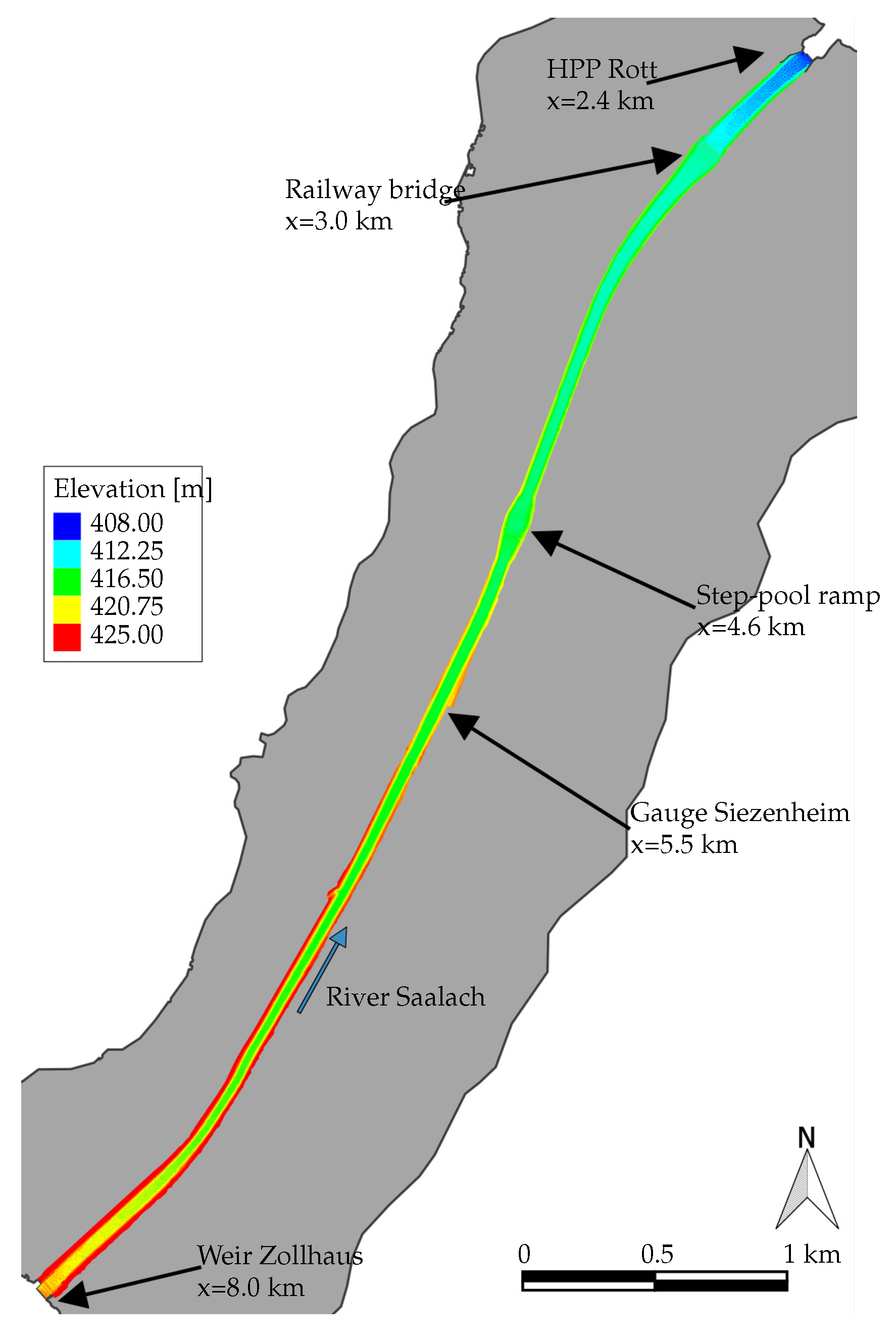
The existing numerical model for simulating inundation areas during the extreme flooding event cover not only the river channel but also wide areas of the surrounding flood plains. Observations of the water elevation in the Saalach River show that at the flow discharges not larger than that used in this study the water remains in the channel. Hence, to decrease the computation time and lower the computational effort, we created a new grid mesh covering only the river channel. The extracted mesh has 24,831 elements, which is only 7.5% of the initial mesh (Figure 4).
As an initial condition used in this study, bed elevation was updated to the possible maximum based on the designed flood protection levees in this region. Further sedimentation causing a higher bed elevation may increase the flood risk and can led to severe inundations (see [26]). Figure 5 shows a longitudinal section of the mean riverbed and the water surface elevation during mean discharge conditions, which serve as the initial condition for the following simulations. Furthermore, the river reach was divided into two parts, an upper free-flowing and a lower reservoir section. The reservoir section can be subdivided again into two areas by a ground sill below a railway bridge at x = 3.0 km, with an averaged crest elevation of = 412.90 m. Upstream of the bridge sedimentation is more critical than usual for flood protection and, at the same time, flushing might not be as effective here as in the lower part because the fixed elevation of the ground sill limits the possible erosion. In addition, at this location the river channel becomes wider, causing a deceleration of the flow (Figure 4).
2.2.3. Boundary Conditions
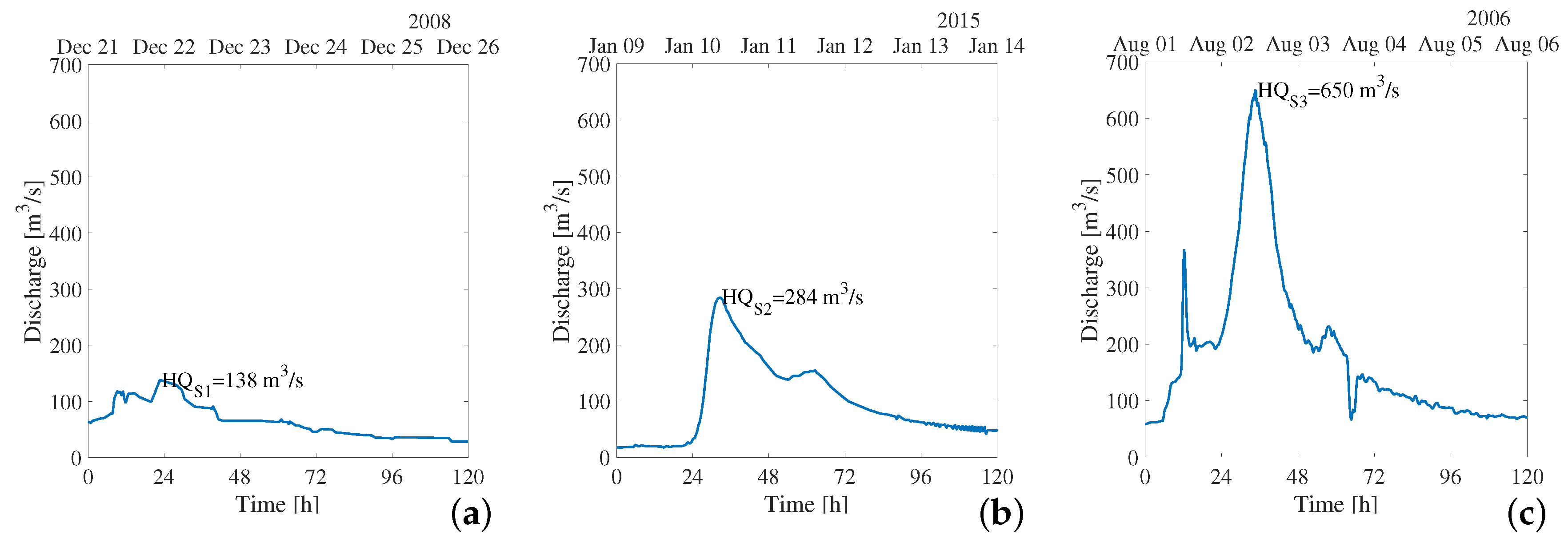
At the inlet boundary, we applied three hydrographs (Figure 6), corresponding to different operation modes. To approximate reality as closely as possible, these hydrographs were selected from the available discharge measurements. The first hydrograph was observed in December 2008, and represents a frequently occurring flow situation, with a peak discharge of HQS1 = 138 m3/s. We selected this case as such small events occur quite regularly and might provide a reliable and predictable regulation option. Moreover, this flow magnitude is around the size of the incipient of sediment motion [27]. The second hydrograph is a medium sized flood event with a peak discharge of HQS2 = 284 m3/s, which occurred in January 2015. Such events occur statistically around once a year. The third scenario investigated focuses on the flushing potential during high floods, such as the event in August 2006, with HQS3 = 650 m3/s. The occurrence of such an event is more uncertain and unlikely, as events with this magnitude have a recurrence probability of around 1/10 per year [26]. This low probability makes such events less suited for planning; however, we expect them to have the biggest potential for sediment remobilisation.
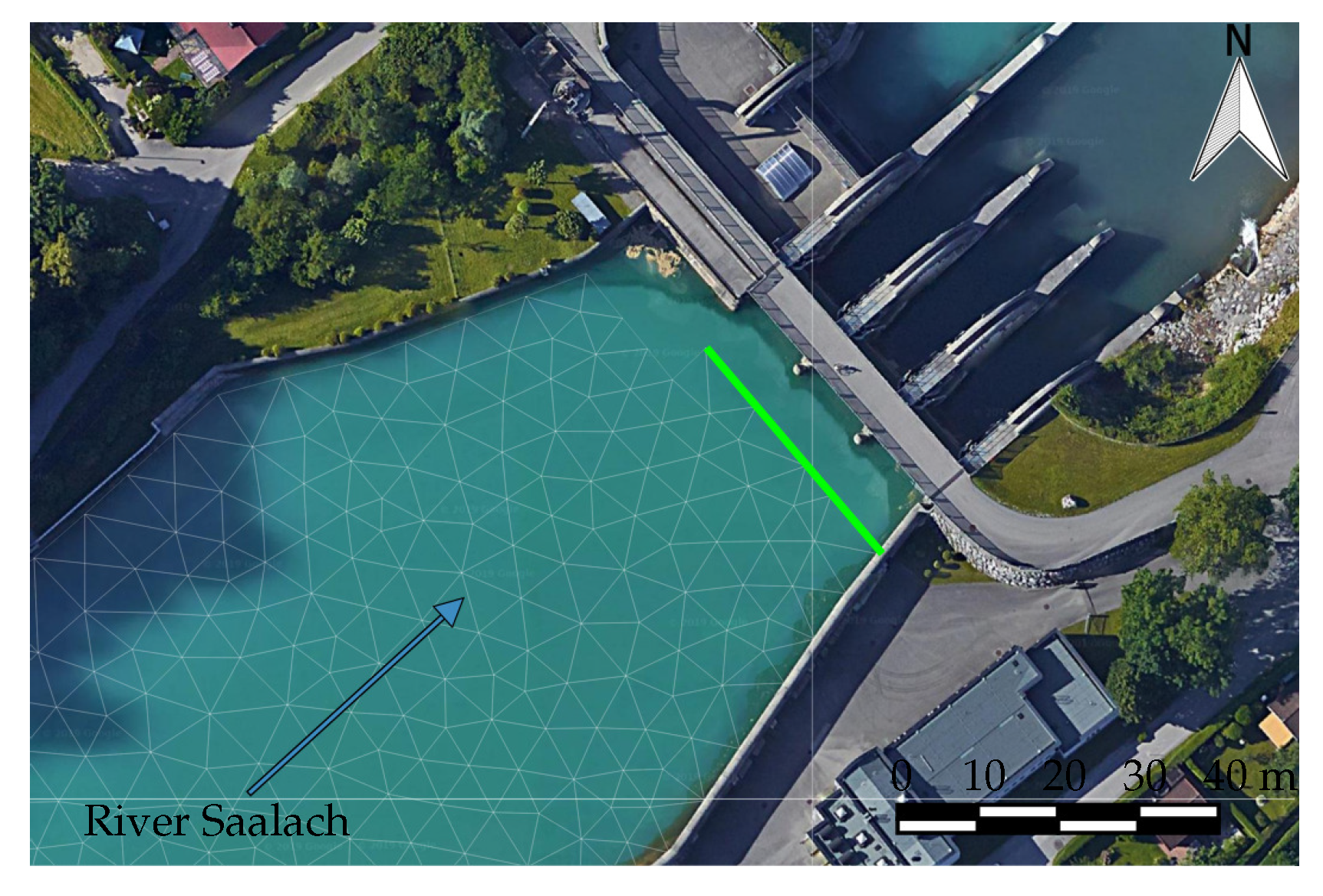
As an outlet boundary condition, the water surface elevation was defined at the HPP. Hence, reservoir drawdown flushing was simulated directly by lowering this water level. Furthermore, we assumed the same water level for all weirs. Figure 7 shows the computational grid at the model outlet, indicating the boundary segments, where water and sediment can leave the domain.
To evaluate sediment-flushing, which is the main objective of this study, we generated four different flushing schemes (denoted as “cases”) for each of the three discharge scenarios. The first case follows the standard hydropower plant operation (Figure 3). In the second case, the water level is defined to obtain free-flow conditions with the completely opened weirs during the simulation time. This case serves as reference case for the others, as the highest mobilised volume is expected here. The transition between storage level Zf,S and free-flow conditions follows the maximum lowering speed of the water level until the corresponding value of the water level from the provided stage discharge condition is reached. The last two cases represent intermediate solutions, to achieve a balance of the sediment output and flushing time.
Finally, we applied the model with a new possible flushing scheme for the time period of eight years from January 2006 to 31 December 2013. The predictions were compared with the observed riverbed (i.e., driven by the real operation scheme) to estimate the plausibility and applicability of the findings.
3. Results
3.1. Investigation of Event Based Flushing
3.1.1. Normal Flow Events
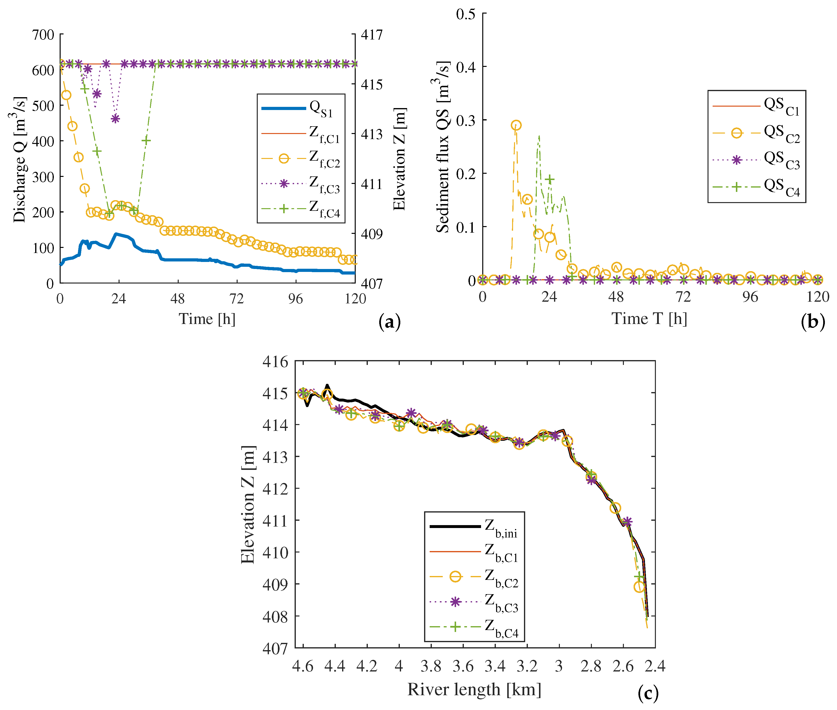
The first scenario is a typical and frequently occurring flow situation. Four different operation cases at the HPP were tested (see Figure 8a). In Case 1, the HPP was operated according to the official regulation scheme, defining in these discharge conditions a constant water level equal to the storage level of Zf,S = 415.80 m. In Case 2, the weirs were opened completely at the beginning of the simulation, allowing free-flow situations in the reservoir. This lowering will take 12 h until free-flowing conditions are reached. For Case 3, the water level is lowered if the discharge exceeds 100 m3/s and raised again when the discharge falls below 100 m3/s. As the peak discharge is only slightly higher than this threshold, and the discharge curve includes some oscillations, the time at lower water level is very short, and thus the water level is only lowered by around 2 m. For Case 4, we simulated a situation with a free-flow condition at the HPP during high discharges. The water level was lowered when the discharge exceeded 100 m3/s (at time t = 20 h). At time t = 31.25 h, the discharge became lower than 100 m3/s again and refilling of the reservoir started.
Figure 8b shows the simulated sediment flux leaving from the domain, and Figure 8c the resulting mean riverbed of the reservoir in a longitudinal perspective. The overall effectiveness of the flushing is given in Table 2, where the total mobilised volumes Vf and the flushing duration tf are provided. During this flow condition, only a limited amount of bed sediment was mobilised. In Case 1, no sediment leaving from the domain was obtained because the weirs were not open, and, in addition, almost no sediment relocation occurs. In contrast, Case 2, under the free-flow condition, provided the highest volume of sediment leaving from the reservoir (10,240 m3). For Case 3, the sediment flux at the outlet boundary was zero again. This shows clearly that the resulting forces on the riverbed were low if the water level was not or only slightly lowered. The flushing in Case 4 required 31 h in total, but, during the free-flowing condition (Case 2), a greater amount of sediment was mobilised.
3.1.2. Medium Flood Events
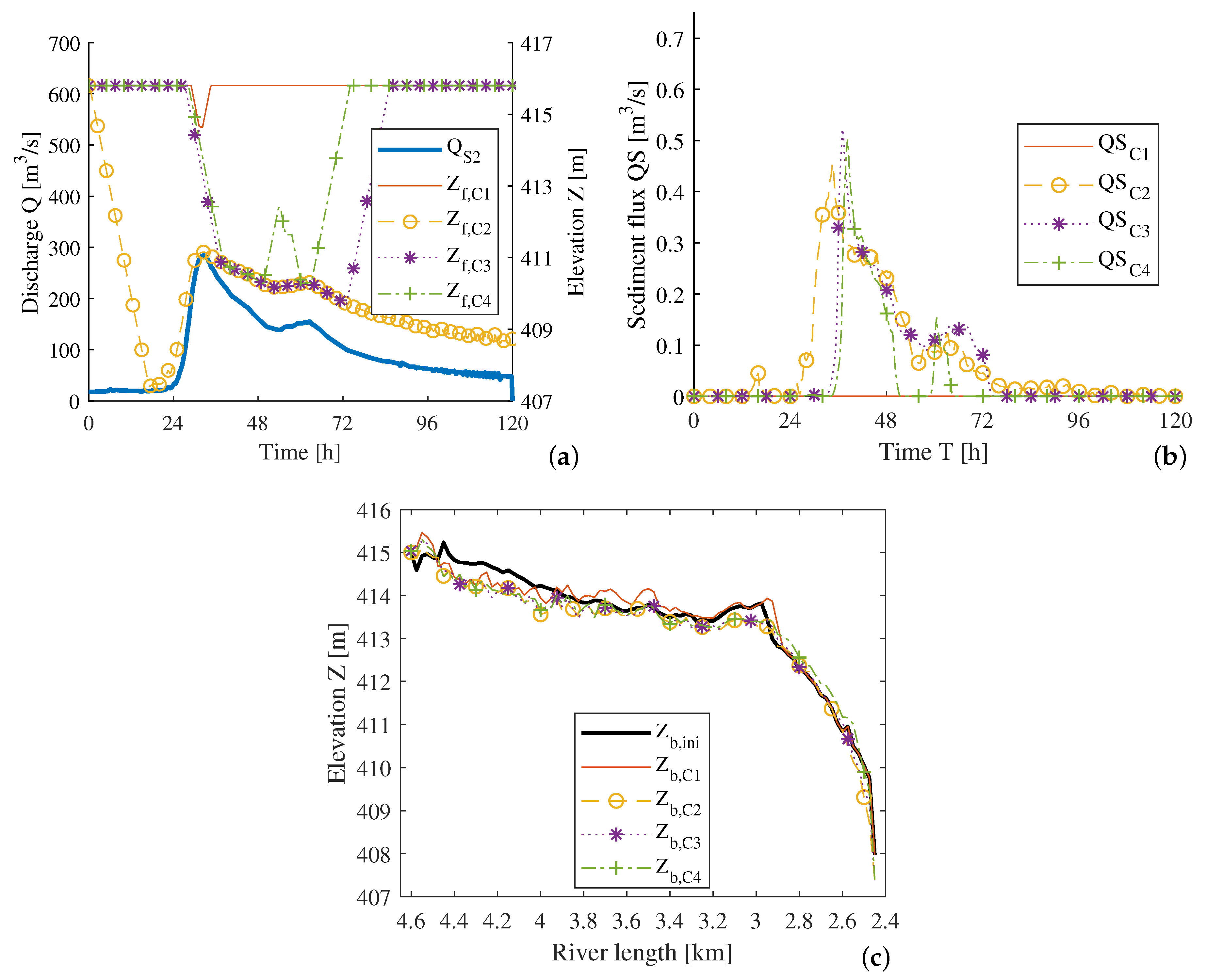
The second scenario investigated was based on a flood event with a peak discharge of Q = 284 3/s, as mentioned above, a size which occurs frequently. Similar to the normal flow event, we created four possible weir operation schemes, where Case 1 followed the official regulation. In Case 2, a completely opened weir was simulated, and in Case 3 the water level was lowered if the discharge was higher than 100 m3/s, leading to free-flow conditions after 11 h at a water level of Zf = 410.9 m. In Case 4, the water level was lowered if the discharge was higher than 150 m3/s and thus after 10.25 h free-flow conditions were obtained. However, due to the shape of the hydrograph in this scenario, which consists of a secondary, smaller peak of Q = 154 m3/s at t = 62.25 h, an intermediate increase and lowering of the water level occurred in Case 4. The time series of the discharge and the water elevation for the four operation schemes are shown in Figure 9a.
Figure 9b shows the sediment flux at the outlet boundary for each case, and Figure 9c shows the resulting riverbed level after the event. Additionally, in Table 3, the total flushed volumes are listed with the necessary time. Following the official weir regulation scheme (Case 1), only local relocation of sediment occurred in the upper reservoir section from x = 4.6 − 3.0 km, but no sediment transported through the outlet boundary was observed. In the second case, around Vf,2 = 32,060 of sediment were flushed out over a time of tf,2 = 120 h, leading to a clear lowering of the riverbed. Case 3 took only around 50% of the opening time tf,2, but during this time around 78% of Vf,2 were still flushed. Moreover, the simulation showed that in Case 4 the flushing was interrupted due to the refilling process, and eroded material in the upper reservoir section was deposited downstream of the railway bridge again, leading there to a higher riverbed and consequently to a lower amount of sediment transported through the domain.
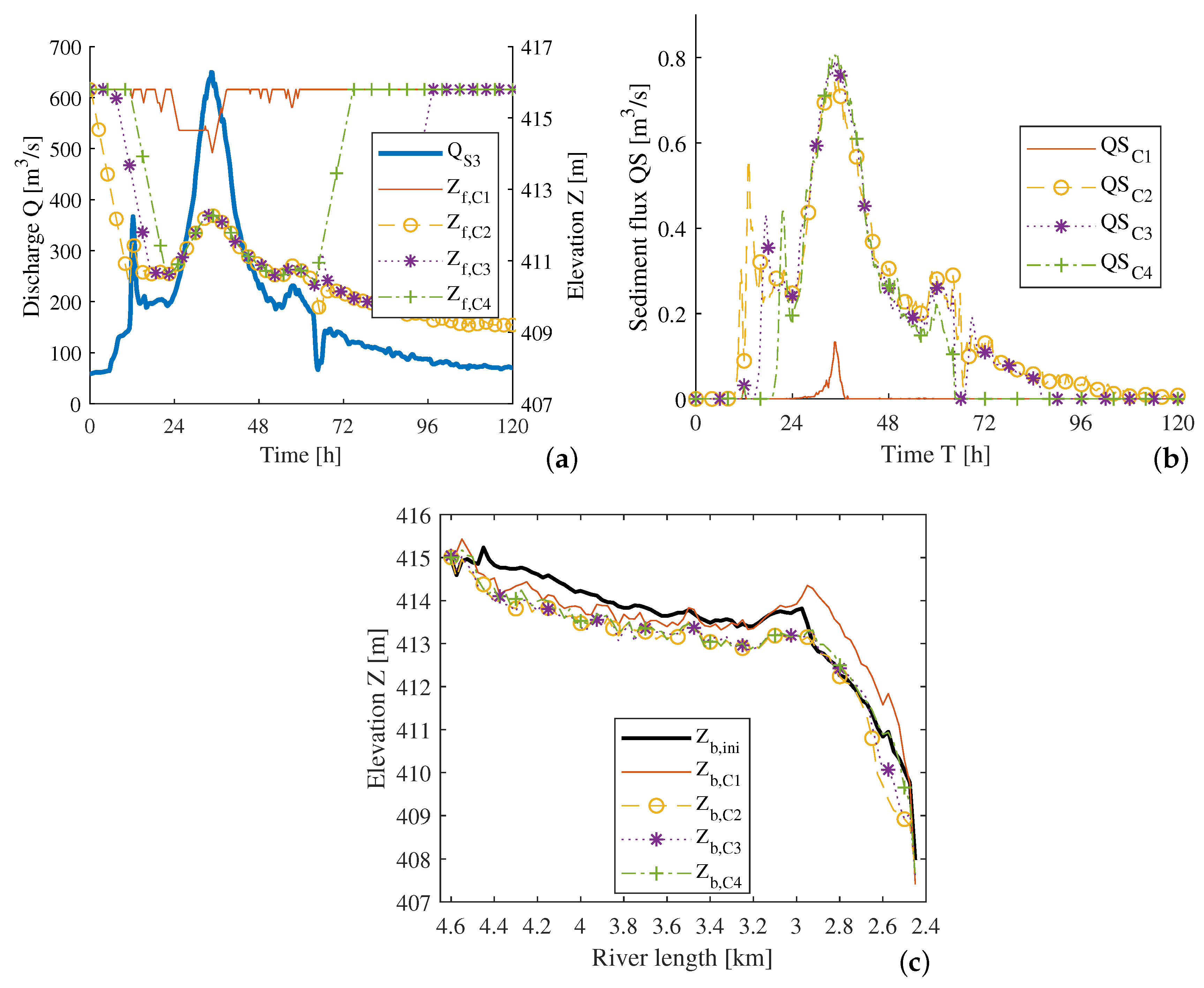
3.1.3. Extreme Flood Event
During extreme flood events, we expected the greatest hydraulic forces on the riverbed and thus very effective flushing. Again, four cases were investigated and compared, as shown in Figure 10a. The first case followed the official weir regulation, leading to a stepwise lowering of the weirs to a level of 414.65 m. The second case shows the situation for the free-flow condition. In the third case, the weirs were opened completely if the discharge Q = 100 , which happened at t = 7 h and lasted until t = 85 h, followed by the refilling of the reservoir. The fourth case used a higher threshold of Q = 150 than in Case 3 in order to see the effect of a shorter flushing.
The simulation results are provided in Figure 10b,c and Table 4. In the first case, only Vf,1 = of sediment was flushed, limited by a too short weir opening time and the partial lowering of the water level. Here, only material in the upper section was eroded, but was then deposited downstream before the HPP. Alternatively, a complete opening of the weirs led to an overall erosion of the riverbed and a volume of Vf,2 = of sediment was transported through the HPP. To optimise the opening time, and thus shorten the time without energy production, we investigated two further cases. The simulated flushing considered discharge regimes over 100 and , leading, as expected, to smaller flushing volumes than in Case 2, but a similar morphological development. The riverbed in the upper section was clearly lower after the flushing and the eroded material was not deposited in front of the HPP.
3.2. Scenario Application
Based on the analysis of the simulated results for different scenarios in Section 3.1, we developed a flushing scheme for the study domain. The simulations were conducted for the period from 1 January 2006 to 31 December 2013 on the original calibrated mesh from Ref. [16]. This is necessary as in this period the 2013 flood event occurred and the floodplain must be included (Figure 4). This allowed us a direct comparison with management actually effected, and with the strategy presented in Ref. [16], where a first draft of a modified weir operating regulation was discussed.
In reality (with the real HPP-operation), during this time period, complete drawdown flushing was carried out four times, and partial lowering of the water level eight times. For a time period of 22 days, the water level was lowered on purpose to re-mobilise sediment, which is about 0.8% of the total time (2921 days). Due to the damage caused by the 2013 flood event, the water level after this event was, in contrast to usual practice, kept lower than the storage level for an additional period of 112 days.
Based on the first draft proposed by Reisenbüchler et al. [16], the weirs should be opened, and thus flushing performed, when the discharge is higher than 250 m3/s. This means for this period of eight years the water surface should have been kept at the designated storage level and the weirs been opened, allowing sediment to pass for a total time period of 30 days (1.1%).
However, based on the results presented in Section 3.1, the total sediment volume transported through the river reach can be increased by an optimised flushing time, starting by lowering the weirs earlier and keeping them open longer than the length of flood wave. We therefore, tested different flushing schemes considering the sediment balance in the reach. The obtained results thus far indicate that flushing is effective when the discharge exceeds 100 m3/s and the free-flowing condition is obtained. The total flushing time tf would be increased by an additional 15 days (about 1.6% of the total time).
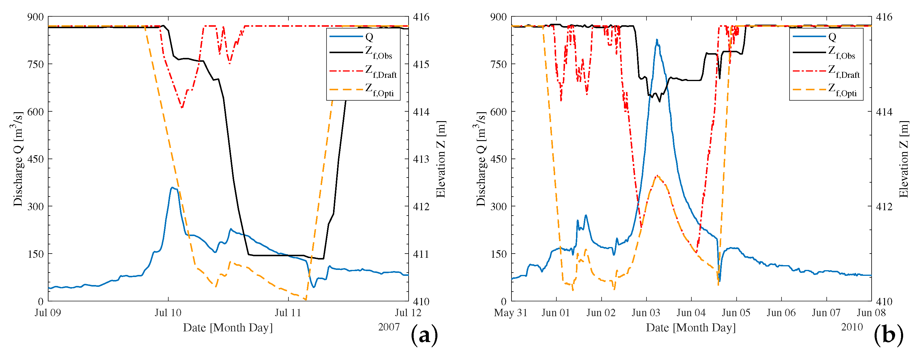
The effectiveness of three operation schemes (the real HPP-operation, the draft scheme proposed by Reisenbüchler et al. [16] and the new proposed scheme) was evaluated considering the flushing parameters. Figure 11 shows the flow discharge at the inlet and the corresponding water levels Zf at the reservoir outlet at x = 2.4 km for two selected flood events. From the observed data (for the real HPP-operation), it can be seen that the water level was lowered when the flood peak had already passed through the inlet boundary in the first example (Figure 11a), while, in the second example (Figure 11b), the water level was only slightly lowered during the flood peak and no real flushing performed. Following the draft scheme, the threshold discharge of 250 m3/s for flushing operations applied only for large floods. However, following the new proposed scheme, the water level would also be lowered for small floods and the weirs kept open longer.
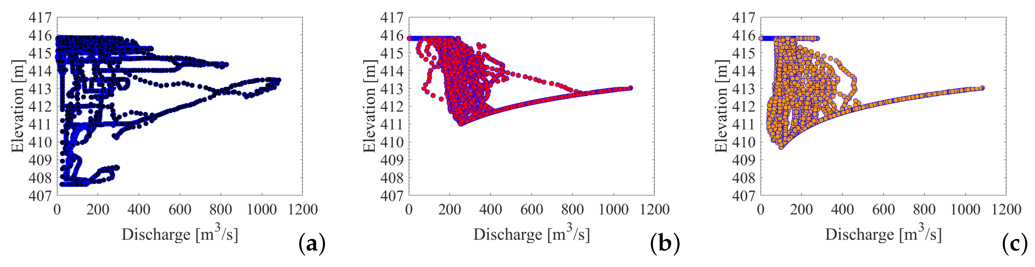
Figure 12 provides a stage-discharge relation at the outlet boundary for the three schemes during the study period. In all schemes, the designated storage level of ZS = 415.80 m can be detected for a wide range of discharges. Moreover, Figure 12a shows the unusual opening after the 2013 flood event, as mentioned above, leading to the low water levels down to an elevation of 408 m. In the proposed and draft schemes is Figure 12b,c, the selected thresholds of 250 m3/s and 100 m3/s respectively, are visible as starting points for free-flowing conditions. To define the lowering water level, both the flow discharge and the maximum lowering speed were considered.
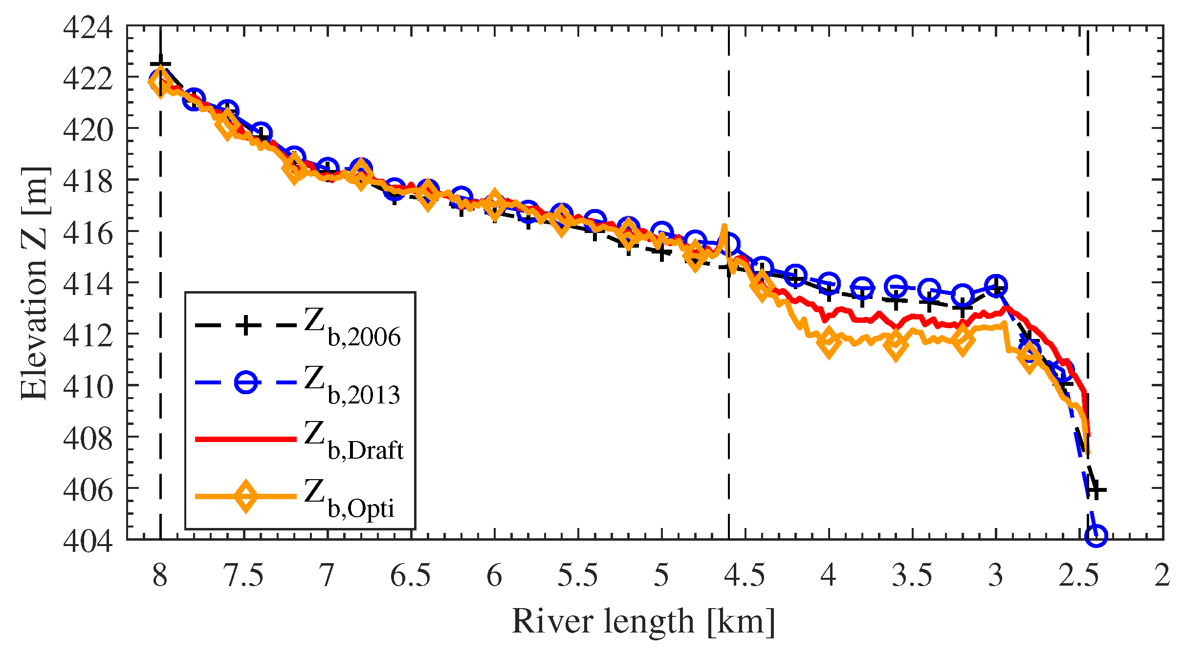
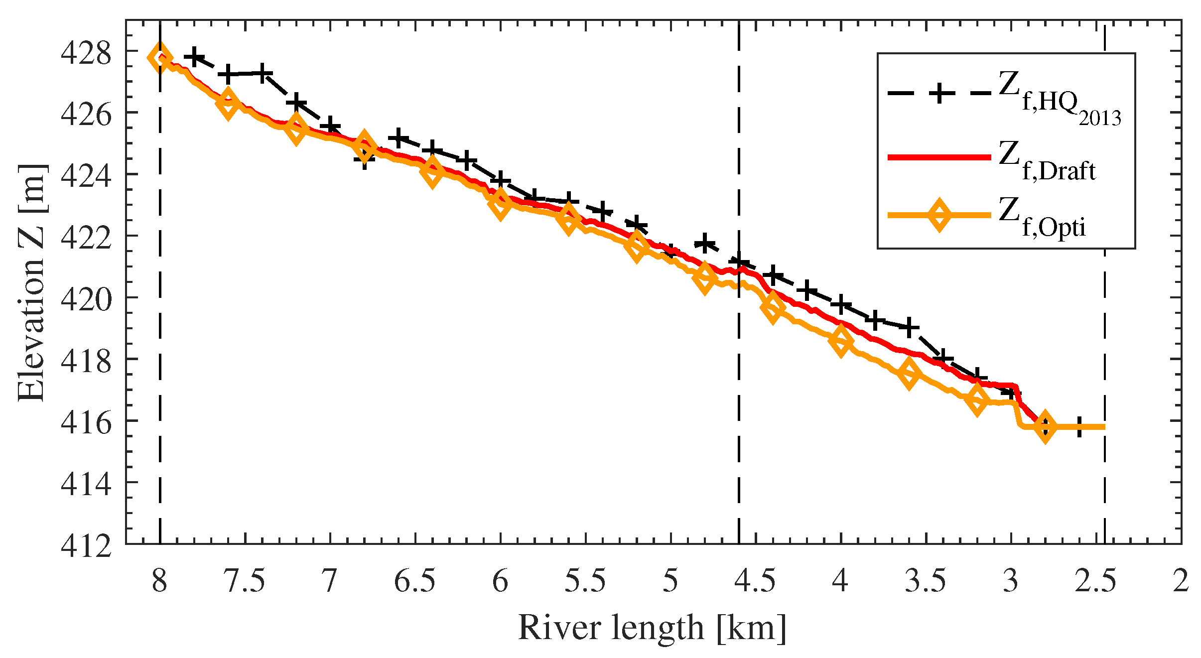
Figure 13 presents the calculated mean riverbed levels along the river reach. Starting from an identical bathymetry based on the observed riverbed in 2006 (as mentioned in Section 2.2.2), both proposed flushing schemes led to a clear lower riverbed in the reservoir section, compared with the measured riverbed in 2013. Increasing the flushing time (+0.5%) in the optimised case (the new proposed scheme) led to a lower riverbed elevation than that obtained by the draft case. Analysing the sediment amount transported through the river reach shows a volumetric difference of about 10,000 m3 at the end of the simulation period between the draft scheme and the optimised one, which is around 1/4 of the annual expected influx of material in the reservoir. In the upper section of the river reach, the free-flowing section, the different operation schemes have no influence and show identical results.
Moreover, despite the increase of re-mobilised sediment, and thus the re-establishment of the sediment continuity, an additional benefit can be created. During the 2013 flood event, extreme high water surface levels were recorded on 2 June 2013 (see Figure 14), causing large inundation and extensive damage [5]. The simulation showed that, with adaptations in the weir regulation, leading to lower bed levels, the water level during this extreme event could also have been lower. In the case of the draft scenario, the reduced water elevation would be around −0.5 m at the most critical section at x = 3.5 km. For the optimised case proposed here, the decreasing of water elevation would be 1.0 m.
4. Discussion
The results of this study, obtained by numerical 2D simulations, provide insight into the processes during drawdown flushing at run-of-river HPPs in gravel bed rivers. For this study, a 2D modelling approach is sufficiently accurate, as Reisenbüchler et al. [5] showed that the differences in the flow velocity between 3D and 2D simulations are very low for this reservoir.
Smaller flood events with a peak discharge lower than HQ1, which were investigated in the first scenario, can mobilise only a low amount of sediment. The results indicate that a complete opening over 120 h, is not an efficient measure as in Case 4 around 70% of the maximum volume Vf,2 is still transported but needs only 25% (=30 h) of the time tf,2. Considering the predicted sediment transported from the river reach with the expected annual average sediment entering the reservoir (approximately 40,000 m3/year) shows that such small events have only a minor impact and do not greatly lower the riverbed. Finally, we classify the simulated processes during this flow scenario more as relocation than real flushing. The reason for this is mobility of the coarse gravel bed of the Saalach, which requires higher hydraulic forces induced by higher shear stresses than during this flow situation.
Sediment-flushing during a medium flood event is a more suitable option for the Saalach River. During such discharges, higher amounts of sediment are mobilised and leave the domain. However, here, the flushing duration plays an important role. If this time is too short, e.g., due to early refilling, re-mobilised sediment from upper reservoir sections is deposited again before it can leave the domain. We estimated that such events could efficiently mobilise up to 25,000 m3 of sediment, which is more than 60% of the annual average sediment input.
As expected, the simulations confirmed that an extreme flood discharge has the greatest potential for sediment-flushing, which mobilised volumes clearly higher than the annual input. Moreover, it is clear that free-flowing conditions during the flushing are much more effective regarding sediment output than only partial lowering of the water level (e.g., down to Zf = 414.65 m). We also observed that in all cases longer flushing led to higher sediment output given a sufficient discharge intensity.
Based on the simulated results in the river reach for a period of eight years, we found that a morphologically optimised operational scheme can lower bed levels, raise sediment output rates and improve flood security due to lower water level during an extreme event. It is clear that, without an efficient flushing activity at the HPP, sedimentation will cause severe problems such as flooding in the area and probably require more expensive countermeasures such as dredging. This would require an official agreement for energy production and sediment management. Our proposed flushing scheme can be applied as the basis of more sustainable sediment management in the reservoir.
In the future, we would like to continue our research on reservoir flushing with additional tests, such as the comparison of the numerical results with a physical model. Through such hybrid modelling approaches, the combination of numerical and physical model can benefit from the strength of both methodologies, as Stephan and Hengl [28] showed, and thus lead to even more reliable results. Moreover, analysis of the data obtained from the numerical simulation could serve as input data for more advanced data processing tools such as artificial neural networks [29,30,31]. Furthermore, we plan to continue this study to assess the impact of reservoir flushing on downstream sections of the reservoir, which we expect due to the flushing alterations of the downstream morphology and ecology, as discussed by the authors of Ref. [7,32,33,34,35]. A possible methodology for such an investigation is presented in Ref. [36].
5. Conclusions
Our numerical hydromorphological model is suitable for optimisation of reservoir operations and developing a sediment management strategy. By testing different reservoir operation modes, we showed that, under certain conditions, sediment could be more effectively re-mobilised and transported through the HPP. However, not all the cases investigated showed the desired effect. We found that, due to the coarse gravel bed of the Saalach River, low flow forces could not mobilise greater amounts of sediment, but led only to local relocation of sediment along the reach. One additional finding is that the flushing time, when the water level is lowered and the weirs are open, is an important factor. This time should be sufficiently long for two reasons: first, to obtain free-flowing conditions during the flushing, which are more effective than only partial lowering of the water level; and, second, to ensure that material which is mobilised by the flow in upper reservoir sections has enough time to pass the weirs at the HPP, as otherwise the sediment will remain in the lower section directly in front of the HPP. Application of the developed numerical models can help to determine this necessary time. In addition, we demonstrated that reservoir management can play an important part in integrative flood management strategies. Applying proposed operation scheme, the water levels in the domain could be reduced, thus providing higher flood security for local residents and settlements. This clearly shows that investigations into sediment management strategies can be a valuable solution to develop integrated flood protection system in combination with technical and ecological measures.
Author Contributions
M.R. designed the study, processed and analysed the data, interpreted the results and wrote the paper. M.D.B. and P.R. contributed to the model development stage with theoretical considerations and practical guidance, assisted in the interpretations and integration of the results and helped in preparation of this paper with proofreading and corrections. D.S. provided expertise on the site-specific conditions, organised the data collection and assisted in the interpretations. All authors have read and agreed to the published version of the manuscript.
Funding
This research received no external funding.
Acknowledgments
The authors are grateful to the Leibniz-Computing-Center (LRZ) for providing the hardware to conduct the simulations.
Conflicts of Interest
The authors declare no conflict of interests.
Abbreviations
The following abbreviations are used in this paper:
| HPP | Hydropower plant |
| GS | Ground sill |
| masl | metres above sea level |
| Zb | Elevation of the riverbed |
| Zf | Elevation of the free water surface |
| Zf,S | Storage level |
| Vf | flushing Volume |
| tf | flushing duration |
| 2D | two dimensional |
| 3D | three dimensional |
| QS | Sediment flux |
| Q | Discharge of water |
| HQ | flood peak discharge |
| MQ | Mean discharge |
| MHQ | Mean flood discharge |
References
- Assembly, U.G. Transforming Our World: The 2030 Agenda for Sustainable Development. 2015. Available online: https://www.refworld.org/docid/57b6e3e44.html (accessed on 12 December 2019).
- Schleiss, A.J.; Franca, M.J.; Juez, C.; De Cesare, G. Reservoir sedimentation. J. Hydraul. Res. 2016, 54, 595–614. [Google Scholar] [CrossRef]
- Dams, W.C.O. Dams and Development: A New Framework for Decision-Making; Earthscan Publications Ltd.: London, UK, 2000. [Google Scholar]
- Annandale, G.W.; Morris, G.L.; Karki, P. Extending the Life of Reservoirs: Sustainable Sediment Management for Dams and Run-of-River Hydropower; World Bank Group: Washington, DC, USA, 2016. [Google Scholar]
- Reisenbüchler, M.; Bui, M.D.; Skublics, D.; Rutschmann, P. An integrated approach for investigating the correlation between floods and river morphology: A case study of the Saalach River, Germany. Sci. Total Environ. 2019, 647, 814–826. [Google Scholar] [CrossRef] [PubMed]
- Schleiss, A.; de Cesare, G.; Franca, M.; Pfister, M. Reservoir Sedimentation; CRC Press: Boca Raton, FL, USA, 2014. [Google Scholar]
- Dépret, T.; Piégay, H.; Dugué, V.; Vaudor, L.; Faure, J.B.; Le Coz, J.; Camenen, B. Estimating and restoring bedload transport through a run-of-river reservoir. Sci. Total Environ. 2019, 654, 1146–1157. [Google Scholar] [CrossRef] [PubMed]
- Isaac, N.; Eldho, T.I. Sediment management studies of a run-of-the-river hydroelectric project using numerical and physical model simulations. Int. J. River Basin Manag. 2016, 14, 165–175. [Google Scholar] [CrossRef]
- Isaac, N.; Eldho, T.I. Sediment removal from run-of-the-river hydropower reservoirs by hydraulic flushing. Int. J. River Basin Manag. 2019, 1–14. [Google Scholar] [CrossRef]
- Gallerano, F.; Cannata, G. Compatibility of Reservoir Sediment Flushing and River Protection. J. Hydraul. Eng. 2011, 137, 1111–1125. [Google Scholar] [CrossRef]
- Ateeq-Ur-Rehman, S. Numerical Modeling of Sediment Transport in Dasu-Tarbela Reservoir Using Neural Networks and TELEMAC Model System; Technische Universität München: München, Germany, 2019. [Google Scholar]
- Chaudhary, H.P.; Isaac, N.; Tayade, S.B.; Bhosekar, V.V. Integrated 1D and 2D numerical model simulations for flushing of sediment from reservoirs. ISH J. Hydraul. Eng. 2019, 25, 19–27. [Google Scholar] [CrossRef]
- Bui, M.D.; Rutschmann, P. Numerical modelling for reservoir sediment management. In Proceedings of the Sixth International Conference on Water Resources and Hydropower Development in Asia, Vientiane, Laos, 1–3 March 2016. [Google Scholar]
- Bieri, M.; Müller, M.; Boillat, J.L.; Schleiss, A.J. Modeling of Sediment Management for the Lavey Run-of-River HPP in Switzerland. J. Hydraul. Eng. 2012, 138, 340–347. [Google Scholar] [CrossRef]
- Esmaeili, T.; Sumi, T.; Kantoush, S.A.; Kubota, Y.; Haun, S.; Rüther, N. Three-Dimensional Numerical Study of Free-Flow Sediment Flushing to Increase the Flushing Efficiency: A Case-Study Reservoir in Japan. Water 2017, 9, 900. [Google Scholar] [CrossRef] [Green Version]
- Reisenbüchler, M.; Bui, M.D.; Skublics, D.; Rutschmann, P. Enhancement of a numerical model system for reliably predicting morphological development in the Saalach River. Int. J. River Basin Manag. 2019. [Google Scholar] [CrossRef]
- Weiss, F.H. Sediment monitoring, long-term loads, balances and management strategies in southern Bavaria. In Erosion and Sediment Yield: Global and Regional Perspectives; Walling, D.E., Webb, B.W., Eds.; IAHS: Wallingford, UK, 1996; Volume 236, pp. 575–582. [Google Scholar]
- BMLFUW. Hydrographisches Jahrbuch von Österreich 2015; The Austrian Federal Ministry of Agriculture, Forestry, Environment and Water Management: Vienna, Austria, 2015; Volume 123. [Google Scholar]
- Olsen, N.R.B.; Haun, S. Numerical modelling of bank failures during reservoir draw-down. E3S Web Conf. 2018, 40, 03001. [Google Scholar] [CrossRef]
- Reisenbüchler, M.; Bui, M.D.; Rutschmann, P. Implementation of a new layer-subroutine for fractional sediment transport in Sisype. In Proceedings of the XXIIIrd Telemac-Mascaret User Conference, Paris, France, 11–13 October 2016; pp. 215–220. [Google Scholar]
- Hervouet, J.M. Hydrodynamics of Free Surface Flows: Modelling with the Finite Element Method; John Wiley and Sons: Chichester, UK, 2007. [Google Scholar]
- Villaret, C.; Hervouet, J.M.; Kopmann, R.; Merkel, U.; Davies, A.G. Morphodynamic modeling using the Telemac finite-element system. Comput. Geosci. 2013, 53, 105–113. [Google Scholar] [CrossRef]
- Ata, R. Telemac2d User Manual. Available online: http://www.opentelemac.org/ (accessed on 12 December 2019).
- Tassi, P.; Villaret, C. Sisyphe User’s Manual; EDF: Paris, France, 2014; Volume 6.3. [Google Scholar]
- Hunziker, R.P. Fraktionsweiser Geschiebetransport; Laboratory of Hydraulics, Hydrology and Glaciology (VAW), ETH Zürich: Zürich, Switzerland, 1995; Volume 11037, p. 191. [Google Scholar]
- WWA-TS. Dataset for the Analysis of the Saalach Flood in 2013; WWA Traunstein: Traunstein, Germany, 2013. [Google Scholar]
- Beckers, F.; Sadid, N.; Haun, S.; Noack, M.; Wieprecht, S. Contribution of numerical modelling of sediment transport processes in river engineering: An example of the river Saalach. In Proceedings of the 36th IAHR World Congress 2015, The Hague, The Netherlands, 28 June–3 July 2015. [Google Scholar]
- Stephan, U.; Hengl, M. Physical and numerical modelling of sediment transport in river Salzach. In River Flow 2010; Dittrich, A., Koll, K., Aberle, J., Geisenhainer, P., Eds.; Federal Waterways Engineering and Resarch Institute: Karlsruhe, Germany, 2010; pp. 1259–1265. [Google Scholar]
- Bui, M.D.; Kaveh, K.; Penz, P.; Rutschmann, P. Contraction scour estimation using data-driven methods. J. Appl. Water Eng. Res. 2015, 3, 143–156. [Google Scholar] [CrossRef]
- Ateeq-Ur-Rehman, S.; Bui, M.; Rutschmann, P. Variability and Trend Detection in the Sediment Load of the Upper Indus River. Water 2018, 10, 16. [Google Scholar] [CrossRef] [Green Version]
- Azmathullah, H.M.; Deo, M.C.; Deolalikar, P.B. Neural Networks for Estimation of Scour Downstream of a Ski-Jump Bucket. J. Hydraul. Eng. 2005, 131, 898–908. [Google Scholar] [CrossRef]
- Liu, J.; Minami, S.; Otsuki, H.; Liu, B.; Ashida, K. Environmental impacts of coordinated sediment flushing. J. Hydraul. Res. 2004, 42, 461–472. [Google Scholar] [CrossRef]
- Capra, H.; Plichard, L.; Bergé, J.; Pella, H.; Ovidio, M.; McNeil, E.; Lamouroux, N. Fish habitat selection in a large hydropeaking river: Strong individual and temporal variations revealed by telemetry. Sci. Total Environ. 2017, 578, 109–120. [Google Scholar] [CrossRef] [PubMed]
- Kondolf, G.M.; Gao, Y.; Annandale, G.W.; Morris, G.L.; Jiang, E.; Zhang, J.; Cao, Y.; Carling, P.; Fu, K.; Guo, Q.; et al. Sustainable sediment management in reservoirs and regulated rivers: Experiences from five continents. Earth’s Future 2014, 2, 256–280. [Google Scholar] [CrossRef]
- Reckendorfer, W.; Badura, H.; Schütz, C. Drawdown flushing in a chain of reservoirs—Effects on grayling populations and implications for sediment management. Ecol. Evol. 2019, 9, 1437–1451. [Google Scholar] [CrossRef] [PubMed] [Green Version]
- Tritthart, M.; Haimann, M.; Habersack, H.; Hauer, C. Spatio-temporal variability of suspended sediments in rivers and ecological implications of reservoir flushing operations. River Res. Appl. 2019, 35, 918–931. [Google Scholar] [CrossRef] [Green Version]
Figure 1.
Overview on the study area (Adapted from [5]).
Figure 1.
Overview on the study area (Adapted from [5]).

Figure 2.
Simplified sketch of the HPP Rott: (a) top view, with the upstream reservoir, the weir with gates, and the orographically left located power house with the turbine intake; and (b) longitudinal section through one of the weirs.
Figure 2.
Simplified sketch of the HPP Rott: (a) top view, with the upstream reservoir, the weir with gates, and the orographically left located power house with the turbine intake; and (b) longitudinal section through one of the weirs.

Figure 3.
Stage-discharge-relation at the HPP Rott for the different operation modes and the transition zones.
Figure 3.
Stage-discharge-relation at the HPP Rott for the different operation modes and the transition zones.

Figure 4.
Extension of the original computational grid (grey) and the extracted main channel (colored).
Figure 4.
Extension of the original computational grid (grey) and the extracted main channel (colored).

Figure 5.
Longitudinal section of the initial bathymetry of the Saalach River, representing the maximum acceptable riverbed in the reservoir (black), the water surface level (light blue) during normal mean discharge conditions, and the top edge of the ground sill at x = 3.0 km.
Figure 5.
Longitudinal section of the initial bathymetry of the Saalach River, representing the maximum acceptable riverbed in the reservoir (black), the water surface level (light blue) during normal mean discharge conditions, and the top edge of the ground sill at x = 3.0 km.

Figure 6.
Hydrograph at the inlet boundary: (a) normal flow event; (b) medium flood event; and (c) high flood event.
Figure 6.
Hydrograph at the inlet boundary: (a) normal flow event; (b) medium flood event; and (c) high flood event.

Figure 7.
Computational grid close to the model outlet, highlighting the outflow boundary segments (green). Satellite image from maps.google.com.
Figure 7.
Computational grid close to the model outlet, highlighting the outflow boundary segments (green). Satellite image from maps.google.com.

Figure 8.
Normal flow scenario: (a) boundary conditions for the normal flow discharge and the water surface level of the four cases; (b) simulated sediment flux at the outlet boundary for each case; and (c) longitudinal section of the mean riverbed in the reservoir for initial conditions (black) and the final situation for each case.

Figure 9.
Medium flood scenario: (a) boundary conditions for the medium flood scenario and the four investigated regulation schemes; (b) simulated sediment flux at the outlet boundary for each case; and (c) longitudinal section of the mean riverbed in the reservoir for initial conditions (black) and the final situation for each case.

Figure 10.
Extreme flood scenario: (a) boundary conditions for the extreme flood scenario and the four investigated regulation schemes; (b) simulated sediment flux at the outlet boundary for each case; and (c) longitudinal section of the mean riverbed in the reservoir for initial conditions (black) and the final situation for each case.

Figure 11.
Hydrograph and corresponding water surface levels for sediment-flushing for the observed (black), the draft (red) and the optimised (orange) scheme for two time periods: (a) July 2007; and (b) June 2010.
Figure 11.
Hydrograph and corresponding water surface levels for sediment-flushing for the observed (black), the draft (red) and the optimised (orange) scheme for two time periods: (a) July 2007; and (b) June 2010.

Figure 12.
Stage-Discharge-relation for the three weir operating schemes: (a) observed; (b) draft; and (c) optimised.
Figure 12.
Stage-Discharge-relation for the three weir operating schemes: (a) observed; (b) draft; and (c) optimised.

Figure 13.
Longitudinal section of the riverbed levels: Observed in 2006 () and 2013 (), as well as the result of the draft scenario () and the simulated optimised case ().
Figure 13.
Longitudinal section of the riverbed levels: Observed in 2006 () and 2013 (), as well as the result of the draft scenario () and the simulated optimised case ().

Figure 14.
Longitudinal section of the maximum water surface levels: Observed in 2013 (), and simulated by the draft scenario () and the simulated optimised case ().
Figure 14.
Longitudinal section of the maximum water surface levels: Observed in 2013 (), and simulated by the draft scenario () and the simulated optimised case ().


Table 1.
Numerical model parameters.
| Parameter | Value |
|---|---|
| Timestep | 3 s |
| Riverbed roughness (Strickler) kst | 35 |
| Form roughness (Strickler) kst,r | manually, sectional adapted |
| Bedload transport formula | Hunziker [25] |
| Shields-parameter | 0.04 |
| Active layer thickness | 0.14 m = dmax |
| Number of grain fractions | 8 |
Table 2.
Comparison of the total flushed volume during normal flow event.
| Case | Flushing Duration tf (h) | Flushed Volume Vf () |
|---|---|---|
| 1 | 0 | 0 |
| 2 | 120 | 10.24 |
| 3 | 13.5 | 0 |
| 4 | 31 | 7.05 |
Table 3.
Comparison of the total flushed volume during the medium flood event.
| Case | Flushing Duration tf (h) | Flushed Volume Vf () |
|---|---|---|
| 1 | 5.75 | 0 |
| 2 | 120 | 32.06 |
| 3 | 58 | 25.11 |
| 4 | 46 | 14.82 |
Table 4.
Comparison of the total flushed volume during the extreme flood event.
| Case | Flushing Duration tf (h) | Flushed Volume Vf () |
|---|---|---|
| 1 | 16 | 1.18 |
| 2 | 120 | 81.83 |
| 3 | 90.5 | 72.16 |
| 4 | 63.5 | 59.80 |
© 2020 by the authors. Licensee MDPI, Basel, Switzerland. This article is an open access article distributed under the terms and conditions of the Creative Commons Attribution (CC BY) license (http://creativecommons.org/licenses/by/4.0/).
Share and Cite
MDPI and ACS Style
Reisenbüchler, M.; Bui, M.D.; Skublics, D.; Rutschmann, P. Sediment Management at Run-of-River Reservoirs Using Numerical Modelling. Water 2020, 12, 249. https://doi.org/10.3390/w12010249
AMA Style
Reisenbüchler M, Bui MD, Skublics D, Rutschmann P. Sediment Management at Run-of-River Reservoirs Using Numerical Modelling. Water. 2020; 12(1):249. https://doi.org/10.3390/w12010249
Chicago/Turabian StyleReisenbüchler, Markus, Minh Duc Bui, Daniel Skublics, and Peter Rutschmann. 2020. "Sediment Management at Run-of-River Reservoirs Using Numerical Modelling" Water 12, no. 1: 249. https://doi.org/10.3390/w12010249
Note that from the first issue of 2016, this journal uses article numbers instead of page numbers. See further details here.