Glacial Lake Outburst Flood (GLOF) Events and Water Response in A Patagonian Fjord
by
 , ,
, ,
Lauren Ross
1,* ,
,
Iván Pérez-Santos
2,3,
Brigitte Parady
4,
Leonardo Castro
5,
Arnoldo Valle-Levinson
6 and
Wolfgang Schneider
7 1
Department of Civil and Environmental Engineering, University of Maine, 5711 Boardman Hall, Orono, ME 04469, USA
2
Centro i~mar, Universidad de Los Lagos, Casilla 557, Puerto Montt 4030000, Chile
3
Centro de Investigación Oceanográfica COPAS Sur-Austral, Campus Concepción, Universidad de Concepción, Concepción 4030000, Chile
4
Wastewater Administration, Portland Water District, 225 Douglas Street, Portland, ME 04102, USA
5
Centro de Investigación Oceanográfica COPAS Sur-Austral, Departamento de Oceanografía, Universidad de Concepción, Concepción 4030000, Chile
6
Department of Civil and Coastal Engineering, University of Florida, Gainesville, FL 32611, USA
7
Instituto Milenio de Oceanografía (IMO-Chile), Universidad de Concepción, P.O. Box 1313 Concepción 3, Concepción 4030000, Chile
*
Author to whom correspondence should be addressed.
Water 2020, 12(1), 248; https://doi.org/10.3390/w12010248
Submission received: 3 December 2019
/
Revised: 26 December 2019
/
Accepted: 28 December 2019
/
Published: 16 January 2020
(This article belongs to the Special Issue Effect of Extreme Climate Events on Lake Ecosystems)
Abstract
:As a result of climate change, the frequency of glacial lake outburst floods (GLOF) is increasing in Chilean Patagonia. Yet, the impacts of the flood events on the physics and biology of fjords is still unknown. Current velocities, density, in-situ zooplankton samples, and volume backscatter (Sv) derived from an acoustic profiler were used to explore the response of circulation and zooplankton abundance in a Patagonian fjord to GLOF events in 2010 and 2014. Maximum Sv was found both during the GLOFs and in late winter to early spring of 2010 and the fall and summer of 2014. The increase in Sv in late winter and spring of 2010 corresponded to multiple zooplankton species found from in-situ net sampling. In addition, diel vertical migrations were found during this seasonal increase both qualitatively and in a spectral analysis. Concurrently with zooplankton increases, wind forcing produced a deepening of the pycnocline. Zooplankton abundance peaked in the fjord when the pycnocline depth deepened due to wind forcing and throughout the entire spring season, indicating that mixing conditions could favor secondary production. These results were corroborated by the 2014 data, which indicate that weather events in the region impact both fjord physics and ecology.
1. Introduction
The inevitability of climate change has spurred studies on how earth’s systems respond to a warming planet. One major consequence of climate change is the melting of glaciers and icefields [1,2,3,4], leading to sea level rise. In particular, oceans have risen 10–20 cm over the past century with a recent global mean rise exceeding 3 mm per year [5]. In Chilean Patagonia, glaciers are reacting dynamically to climate change [3]. Specifically, in the Northern Patagonia Icefield, Steffen glacier has lost 12 km2, Glaciar Nef has lost 7.9 km2, and Colonia glacier has lost 9.1 km2 since 1979 [6]. This extreme melting first affects local water bodies, which includes fjords, and subsequently regional fjords and the world’s oceans.
Fjords are glacially carved channels located in high-latitudes where glacial activity is (active glacier) or was (extinct glacier) prevalent [7]. Generally, fjords are long, narrow, and deep with a typical width-depth ratio of 10:1 [8,9] and contain one or several submarine sills (or terminal moraines) that are located along the fjord at the location of ancient glacier terminus [8,9]. Fjords are characterized by their strong salinity-driven stratification (up to 10–20 g kg−1m at the pycnocline) with a thin (~5–10 m) buoyant layer at the surface (~0 g kg−1) derived from glacial melt, river discharge, precipitation, and coastal runoff [9,10,11] overlying a salty dense layer below (~32–35 g kg−1). Mixing between layers results from vertical shears inherent to inflowing saltwater and outflowing freshwater or to internal waves and tidal currents [10].
Ultimately, climate change will alter the above-mentioned water column properties and biology of fjord systems [12,13]. In particular, temperature, salinity, and circulation structure will be impacted by rising ocean and atmospheric temperatures and glacial lake outburst floods (GLOFs) and, in turn, biology will be affected by these altered properties. GLOFs occur when water trapped by a glacial dam is suddenly released due to the dam melting [14,15]. GLOFs occur not only in Patagonia [13,14,15], but also in the Nepal Himalayas [16], the fjords of Norway [17], the Bolivian Andes [18], the Kodar Mountains in Siberia [19], and the Karakoram Mountains in China [1] to name a few, with many occurrences newfound or intensifying due to climate change, causing disastrous flooding and damage of downstream infrastructure.
As a result of increased atmospheric temperatures and ice melt, ice fields in Chilean Patagonia are under accelerated retreat and the frequency of GLOF events is on the rise. Marín et al. (2013) [13] found that the Baker River, one of the largest rivers in Chile in terms of discharge values, experienced a 600% increase in GLOF events between 2010 and 2012, emphasizing the need to fully understand their consequence on both hydrodynamics and biology in Chilean fjords [14,20,21]. In particular, the release of glacial water from GLOFs has been found to alter the surrounding ecosystem as it can lead to increased light attenuation and decreased primary production [13,22,23,24]. On the other hand, these pulses can also deliver nutrients to the fjord, which can increase primary production [25]. Hydrodynamics shall also have a profound impact on zooplankton abundance and distribution, as has been found on a large scale by Klevjer et al., (2016) [26] in the North Atlantic, Indian, West Pacific and East Pacific oceans. However, studies linking zooplankton to fjord physical properties are limited, especially in Chilean Patagonia. The few studies on this topic indicate that variations in precipitation and freshwater discharge affect primary and secondary production [11]. Further, changes in freshwater input will ultimately alter fjord stratification, which contributes to spatial distributions of zooplankton [27]. More specifically, phytoplankton dwell in the less saline surface waters and zooplankton ascend from depth to feed on them. This vertical migration pattern is often regulated by light availability. Influxes of sediments and freshwater due to GLOFs can thus alter the vertical distribution and migration patterns of the zooplankton as well as temporarily augment circulation patterns in a fjord [25,28,29].
The main goal of this study is to investigate how physical properties (currents and pycnocline location) of a glacial fjord in Chilean Patagonia affect zooplankton aggregation intra-annually and during GLOF events. This goal is addressed with the following two research questions: (1) How does zooplankton aggregation and migration vary depending on austral season? (2) How do fjord physical properties, linked to zooplankton aggregation, change during a GLOF event? The research questions will be answered using a one-of-a-kind dataset collected over two different years from a Chilean Patagonian Fjord. This study is unique in the availability of river discharge data as well as density, current velocity, volume backscatter (as a proxy for zooplankton distributions), and in-situ zooplankton sampling to describe the hydrodynamic patterns of the fjord and how they link to variations in zooplankton.
2. Materials and Methods
2.1. Study Area
Located in the Southern Hemisphere, Patagonian Chile represents 240,000 km2 of glacially carved land on the southwest coast of Chile [11]. It features a mountainous coastline and complex fjord and channel systems that were glacially carved through the steep slopes of the Andes mountain range. The Northern and Southern Patagonia Ice Fields supply freshwater to the fjords through glacially fed rivers and lakes and represent the largest two bodies of ice in the southern hemisphere.
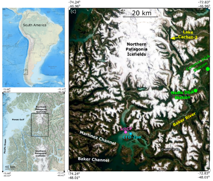
The study area is located toward the southern end of the Northern Patagonian Ice Field in Martinez channel (Figure 1). Between 200 and 440 m deep, Martinez Channel is oriented in the East-West direction and is forced by primarily semi-diurnal tides (~1 m amplitude and period of 12.42 h) [30]. The mouth of Martinez channel (3.5 km wide) connects to the open ocean ~100 km from the head of the system [25]. Freshwater in Martinez Channel is mainly derived from the Baker River with average annual discharge exceeding 1100 m3 s−1 [31]. The freshwater layer is ~5–10 m deep with low temperatures (<8 °C) and low salinity (<30 g kg−1) [32]. Upstream, Colonia glacier forms an ice dam preventing water from Lake Cachet 2 (surface area of 4 km2) from flowing into the Baker River [13] (Figure 1c). Long-term thinning of this glacier has led to an increase in Glacial Lake Outburst Flood (GLOF) events [21]. During a GLOF, meltwater bursts through Colonia Glacier via an englacial tunnel running 8 km in length [21]. From there, it flows through Colonia Lake and the confluence between Colonia and Baker Rivers into Martinez channel. The village of Tortel at the mouth of the Baker River is particularly vulnerable to flooding and having murky water during a GLOF. In addition, the area of Martinez channel is affected by regular synoptic or storm events every ~20–30 days associated with the Baroclinic Annular Mode (BAM) [31]. The BAM storm events are driven by extratropical fluxes of heat from the equator to the Southern or Antarctic Ocean (40–55° S) [32,33,34]. The effect of the BAM on the physics and biology of fjords and channel systems in Chilean Patagonia is only now becoming apparent [31,35]. In fact, Ross et al. (2015) [31] found that the BAM produced periodic winds that deepened the pycnocline and enhanced currents at 25–30 d intervals in Martinez Channel. Perez-Santos et al. (2019) [35] expanded on this study by showing periodic wind influence over the entirety of Chilean Patagonia.
2.2. Data Collected
2.2.1. Acoustic Doppler Current Profiler
In order to investigate the GLOF events, horizontal current velocities, acoustic backscatter measurements, and temperature were obtained with a 307.7 kHz Acoustic Doppler Current Profiler (ADCP Workhorse, Teledyne RD instruments) in Martinez Channel Chilean Patagonia near the Baker River (Figure 1c). The upward pointing ADCP was moored at ~30 m depth at the intersection between Martinez Channel and Stefan Fjord, which directly connects Martinez Channel to the Northern Patagonia Icefield (Figure 1). These data were collected hourly with 120 pings per ensemble and a bin size of 1 m, covering the austral autumn (May–June), winter (July–September), and spring (October–November) seasons of 2010. In addition, the same ADCP was moored (facing up) at the same location for the majority of 2014; from 28 January–11 June at 86 m depth, from 11 June–17 December at 82 m depth, and from 17 December–28 December at 96 m depth. The 2014 measurements were collected in 1 m vertical bins every hour with 250 pings per ensemble distributed equally in the hour.
The 2010 data were originally used to study synoptic band pycnocline modulations in Martinez Channel [31]. That study found that pycnocline vertical excursions, indicative of a deepening of the mixed layer, would occur with 20–30 day periodicity, which is in line with the Southern Hemisphere’s baroclinic annular mode (BAM). The present study extends the findings of the previous study to assess how the pycnocline excursions and/or GLOF events affect zooplankton aggregations in Martinez Channel. The 2014 dataset has been used by Meerhoff et al. (2019) [25] to assess the contribution of terrigenous and marine plankton carbon sources to the particulate organic matter in the fjord before and after a GLOF to link to zooplankton abundance. Their study explores approximately 10 days of data surrounding a GLOF event. Our study will expand on the findings of Meerhoff et al. (2019) [25] and Ross et al. (2015) [31] by determining how the physical properties and zooplankton abundances in the fjord vary both during a GLOF and throughout other austral seasons. Our study will also determine the intra- and inter-annual effects of GLOFs on physical and biological properties of the fjord.
2.2.2. River Discharge
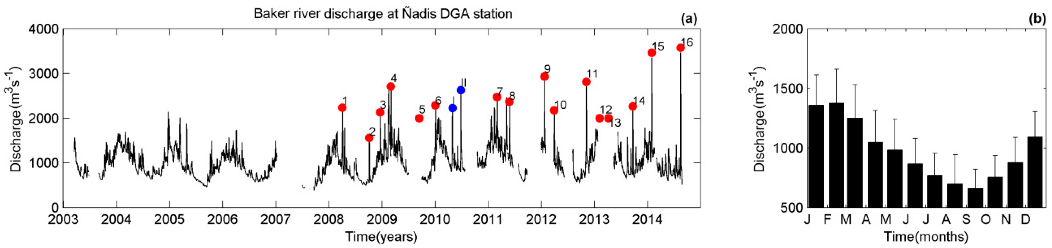
In order to identify GLOF events, Baker River discharge measurements were obtained from the Chilean Water Directorate (Dirección General de Aguas DGA) at two points, the Ñadis (47°30′ S, 72°58.50′ W) and Colonia (47°20.78′ S, 72°51.60′ W) stations (Figure 1). The combination of discharge measurements from these two stations indicate that there have been 16 verified GLOF events and two other possible occurrences since 2008 (Table 1), with an upward trend in intensity of the discharge events from 2003 to 2014 (Figure 2a). The GLOF events show discharge values ranging from ~1500 m3 s−1 to 3500 m3 s−1. The average monthly river discharge varies from ~700 m3 s−1 in the Austral Winter (September) to ~1400 m3 s−1 during Austral Summer (February) (Figure 2b). This study focuses on the fjord response to GLOF II on 29 June 2010 and GLOF 15 on 1 February 2014, as instrumentation was deployed in the fjord system during these events. During 2010, river discharge measurements were only available at the Colonia station and not Ñadis station. By 2014, river discharge data were also available at Ñadis station.
2.2.3. Salinity and Temperature
Hydrographic data including temperature, salinity, density, chlorophyll, and dissolved oxygen were collected in Martinez Channel using a SeaBird Electronics 19 plus Conductivity, Temperature, Depth (CTD) profiler in 2014 (see Supplementary Material). Vertical casts ~100 m deep were collected at the junction between Martinez Channel and Steffen Fjord (Figure 1c, 46°49.30′ S, 73°37.30′ W). CTD casts were taken in January, June, November, and December of 2014. These measurements provide an overview of hydrographic properties of the fjord in the austral seasons. Density profiles from 2010 are presented in [31] and show similar features to those of the 2014 data.
2.2.4. Zooplankton Sampling
In-situ zooplankton samples were collected monthly adjacent to the ADCP mooring in 2010 (Figure 1c). This was accomplished with a Bongo net towed from 25 m depth to the surface (60 cm mouth opening, 300 µm mesh, flowmeter mounted in the net frame) [27]. All samples were preserved in a 5% formaldehyde solution [36,37]. At the laboratory, the zooplankton samples were identified and separated into major functional groups and organisms ≥5 mm in size (detectable size for 307.7 kHz ADCP) were classified to the lowest taxonomical level. Zooplankton abundances were standardized to individuals per 100 m3 of filtered seawater [38].
2.3. Data Analysis
The echo intensity (backscatter) from the ADCP is measure of the sound scatter off of particles suspended in the water column. The echo intensity was corrected for attenuation of the signal by removing the time mean profile as was done by Valle-Levinson et al. (2004) [39] and explained in Rippeth and Simpson (1998) [40]. The resulting echo anomaly time series is a normalization of the echo intensity and can be used as a proxy for pycnocline location, as sediments tend to accumulate there, and for indicating the presence of other suspended particulates.
The concentration of plankton species within the water column can be estimated from volume backscattering strength recorded at multiple sound frequencies [41]. The ADCP backscatter signal was converted to the mean volume backscattering strength (Sv, dB re 1 m−1) using the relationship:
where, C is a sonar-configuration scaling factor (-148.2 dB for the Workhorse Sentinel), Tx is the temperature at the transducer (°C), LDBW is 10log(transmit-pulse length in meters), and the transmit pulse length was found to be L = 8.13 m. PDBW = 15.5 dB re 1 W is 10log (transmit power, in dB re 1 W), is the absorption coefficient (dB m−1), Kc is a beam-specific sensitivity coefficient (supplied by the manufacturer as 0.45), E is the recorded automatic gain control (AGC), and Er is the minimum AGC recorded (54 dB). The beam-average of the four transducers was used to quantify the Sv to minimize the signal to noise ratio following the procedure in [42]. Finally, R is the slant range to the sample bin (m), and as discussed in Lee et al. (2004) [43]. This value should use the vertical depth as a correction and is obtained with the following equation:
where b is the blanking distance (3.23 m). The variable L is the transmit pulse length (m), which is the same as that used in Equation (1). The variable d is the length of the depth cell (1 m), n is the depth cell number of the particular scattering layer being measured, ζ is the beam angle (20°), is the average sound speed from the transducer to the depth cell (1453 m s−1), and is the speed of sound used by the instrument (1454 m s−1).
As the frequency of the acoustic instrument increases the detectable zooplankton size decreases, e.g., a 720 kHz acoustic device can detect animals with a ~1.5 mm diameter in a water column ~30 m deep. On the other hand, with lower frequencies, e.g., a 120 kHz, a water column ~200 m deep can be studied and animals with a ~10 mm diameter can be measured [44]. A 307.7 kHz ADCP was used in this study. This frequency ADCP can detect animals with a diameter of ~5 mm [23].
Spectral and wavelet analyses were used to determine the dominant frequencies found in the time series of Sv and the echo anomaly depending on austral season. The spectral analysis [45] was used as a first attempt to identify diel vertical migrations of zooplankton and tidal signals in the time series. The spectral analysis was implemented on the time series of Sv and/or the echo anomaly at each depth bin by applying a Fast Fourier Transform (FFT) to the data, window averaging (at least 21 Hanning Windows) allowing for at least 84 degrees of freedom [45]. The wavelet analysis [46] expands upon the spectral analysis by determining the temporal variability of the diel signal as well as the depths at which the diel signal was most pronounced. A 4th order Morlet Wavelet was applied to the time series of the echo anomaly for the 2014 dataset at each depth bin of the ADCP. Then, the energy at the diurnal band (~22–26 h) only was extracted from the Wavelet performed at each depth following the methodology of Torrence and Compo (1998) [46]. Isolating the diurnal energy with depth allowed the times and depths at which diurnal signals were found to be linked to zooplankton vertical migrations. A similar wavelet analysis was carried out in [32] to identify semidiurnal internal tides in Martinez Channel, Chile and the reader is referred to their paper as well as [46] for further details regarding the analysis.
3. Results
3.1. Volume Backscatter, River, and Zooplankton in 2010
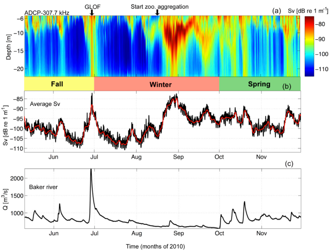
The time series of Sv from 2010 showed highest values (~-75 dB) from mid-winter (Austral winter months: July, August, and September) to spring (October and November) of 2010 (Figure 3a), indicative of higher abundances of zooplankton in the fjord and/or the development of a mixed layer during these months. In addition to elevated Sv values during Austral Winter to Spring, they were also observed at the end of the Fall season (>-85 dB re 1 m−1; Austral autumn months: May and June), with a coherent signal from the surface to 25 m depth, indicating an increase in scatterers at this time.
Baker River discharge measurements from Colonia station (Figure 1b) were obtained during the same time period as the ADCP deployment (Figure 3c). Throughout this time series (autumn-spring of 2010), freshwater input from the Baker River varied primarily from Q = 500 m3 s−1 to Q = 1200 m3 s−1, with a clearly defined maximum of Q = 2228 m3 s−1 at the end of June, 2010. This maximum was due to a GLOF event from the Cachet 2 Lake located to the northeast of the study area (Figure 1b). This event was evident in Sv as the high acoustic signal (>-85 dB re 1 m−1) at the end of June 2010 (Figure 3a,b). In order to determine the impact of pycnocline depth and GLOF events on zooplankton, in-situ zooplankton samples were collected each month of 2010.
3.1.1. Seasonal Changes in Zooplankton
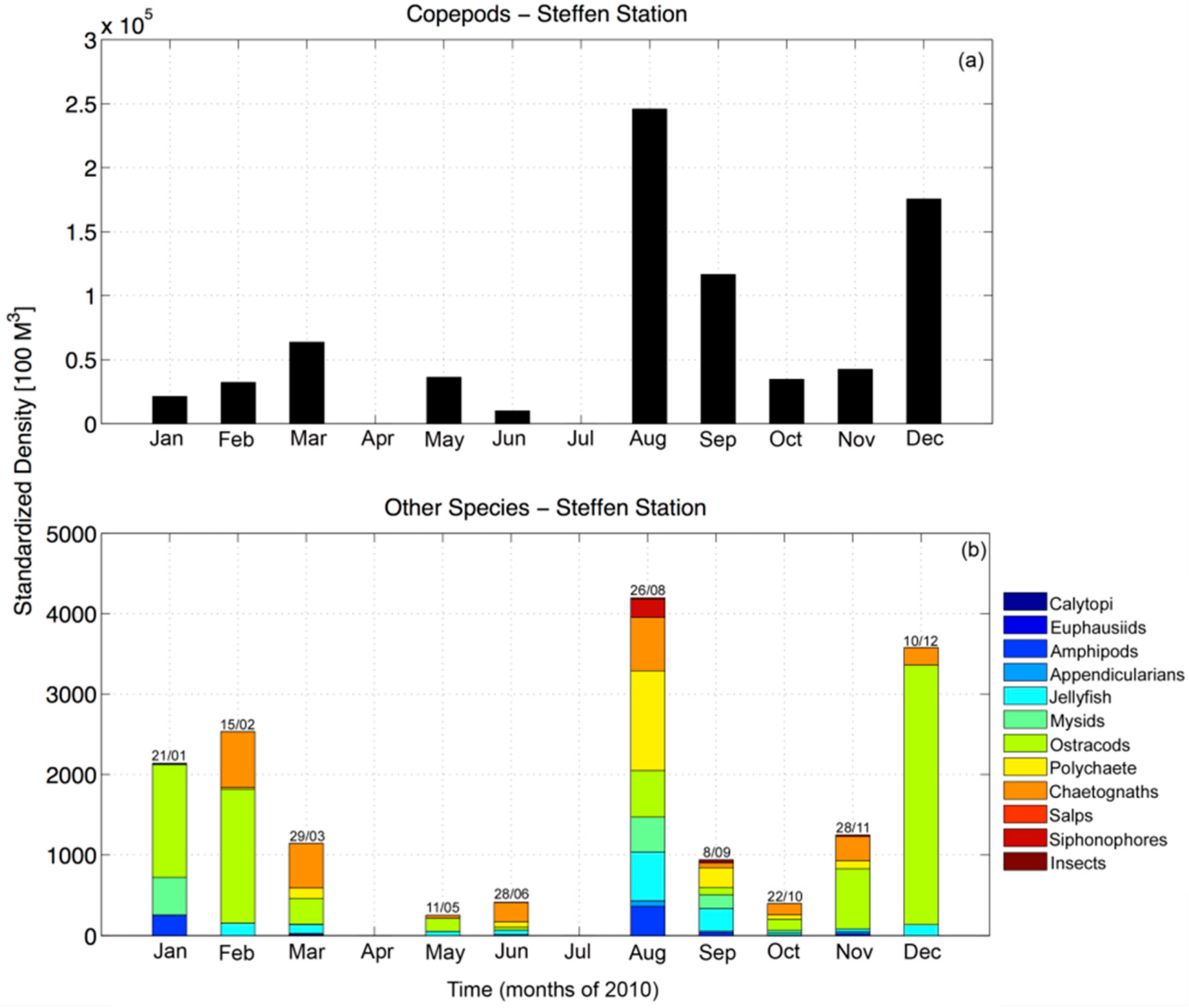
In-situ monthly zooplankton samples collected in Martinez Channel in 2010 confirmed that peak zooplankton abundance appeared in late August to early September occurring concurrently with Sv maxima (Figure 3 and Figure 4). Copepods were consistently the most abundant organisms, with other zooplankton groups such as siphonophores, chaetognaths, and polychaete larvae present, but in lower abundance. In June and July, when GLOF II occurred, the overall zooplankton abundance was much lower than at the end of austral winter and spring. These measurements were only taken during one day of each month, implying that they could not be representative of the entire month. Therefore, we again turn to Sv to propose the variability of zooplankton aggregation during each austral season.
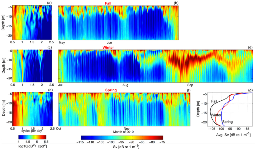
We examined the volume backscatter, Sv, by season and via spectral analysis on the seasonal time series at each depth bin. The spectra revealed diurnal peaks that penetrated down to the depth of the instrument (Figure 5). Semidiurnal peaks, which were associated with the dominant tidal variability, were restricted to the upper 10 m of the water column in all seasons. Although the austral autumn (June and July) revealed the lowest abundance of zooplankton in the in-situ sampling (Figure 4), and the seasonal average of Sv is the lowest (Figure 5g), the spectra of Sv during these months reveals a peak at the diurnal period. Therefore, diel vertical migrations are still occurring at this time (Figure 5a), as also observed in the instantaneous profiles (Figure 5b). In fact, the banding of the signal displayed in all instantaneous profiles is dominated by diel variability.
3.1.2. GLOF II–29 June 2010
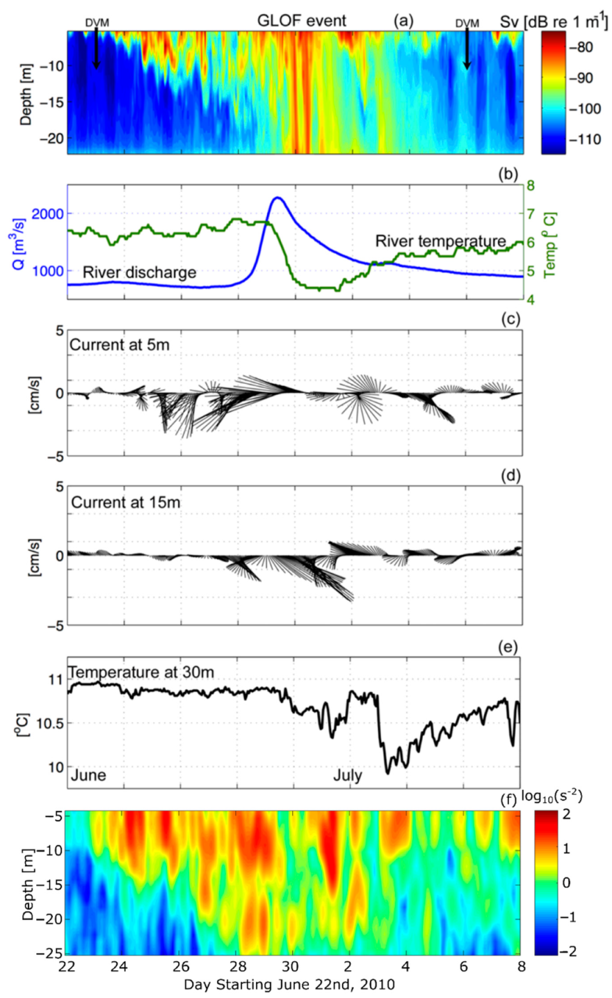
GLOF events occur in Martinez Channel when the Baker River discharge exceeds 2000 m3 s−1 [13]. On 29 June 2010 the Baker River discharge reached 2200 m3 s−1 and the acoustic profiler captured the fjord’s response. A diel signal in Sv was found prior to (22–25 June) and after (4–7 July) the GLOF II (Table 1) event, that was related to diel vertical migrations (DVM) of zooplankton (Figure 6a). Starting on 24 June, Sv increased around the pycnocline (10–12 m) and subsequently became enhanced in both intensity and vertical extent until 4 July. The gradual increase in Sv was suspected to be sediment transported by the start of the floodwaters through the Baker River (Figure 6b). There was a slight increase in river discharge on 23 June and a ~0.5° drop in temperature in the river, which indicated that the ice dam could have weakened on the 23rd. Weakening of the ice dam let some of the floodwaters escape. Full release (or breaking) of the ice dam occurred on 28 June (Figure 6a,b). By 28 June, river flow increased from 780 to ~2200 m−3 s−1 and the Sv signal became elevated (>-90 dB) from near surface to ~25 m (the extent of the ADCP measurements). The Baker River discharge reached its peak at 09:00 on 29 June and at this time the river water temperature decreased from 6.6 °C to 4.3 °C (Figure 6b). Approximately 13 h after the river discharge peak at Colonia Station, the ADCP recorded increased backscatter associated with riverine suspended material. The flood waters arrived in the fjord at approximately 22:00 on 29 June. A second pulse of enhanced Sv was recorded 8 h later at 06:00 on 30 June with similar features as the first (Figure 6a); however, the river discharge measurements did not spike a second time. This could be due to a second release of riverine water down-stream of the Colonia station; however, this is speculation because discharge measurements were not available farther downstream at this time. On 1 July 2010 the elevated Sv signal from the GLOF II event slowly tapered off but remained apparent throughout the water column until 5 July (4 days later), when the diel vertical migrations of zooplankton were once again recognizable within the water column (Figure 6a).
During the GLOF II event, horizontal current velocity vectors at 5 m and 15 m depth showed vertical shear of the horizontal velocities (flow at 5 m depth was west-northwestward and flow at 15 m depth was southeastward), which could enhance mixing at the pycnocline (Figure 6c,d). In fact, the westward (out-fjord) surface currents (5 m depth) doubled in magnitude during the GLOF II, which favored the transport of sediment from the Baker mouth to the ADCP mooring site. Sub-surface currents (15 m depth) also increased in magnitude, yet were directed eastward (into the fjord), suggesting an enhancement of the gravitational circulation in the fjord during the pulse. This is supported by the enhanced squared vertical shear, , during this time, but especially on 1 July, after the GLOF waters were introduced into the fjord (Figure 6f). The fjord water temperature recorded by the ADCP at 30 m depth dropped ~0.5 °C from 30 June to 2 July 2010 because of the cold water discharge from Lake Cachet-2 during GLOF II. Subsequently, the temperature decreased ~1 °C on 3 July (Figure 6e).
In summary, the 2010 dataset revealed that zooplankton were prevalent in the fjord and maintain diel vertical migration (DVM) patterns year round, although this pattern is more apparent during the austral winter and spring months (August–December) than the austral autumn (June and July). Further, the DVM involve zooplankton ascending to the pycnocline, which can act as a barrier during times of strong stratification. When the pycnocline deepens and weakens because of mixing (for example, during austral winter months), zooplankton can be prevalent throughout the water column. One possibility is that the deepening and weakening of the pycnocline makes phytoplankton, thriving in the fresh surface layer, easy prey for the zooplankton. Increased zooplankton abundance will augment the already elevated Sv signal during these times of pycnocline weakening and deepening. A similar dataset collected in 2014 is described next to determine if the findings from 2010 are repeatable.
3.2. Density, Volume Backscatter, River, and Zooplankton in 2014
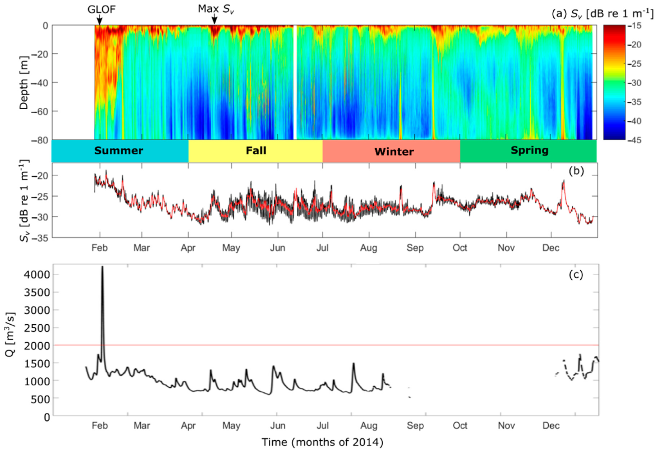
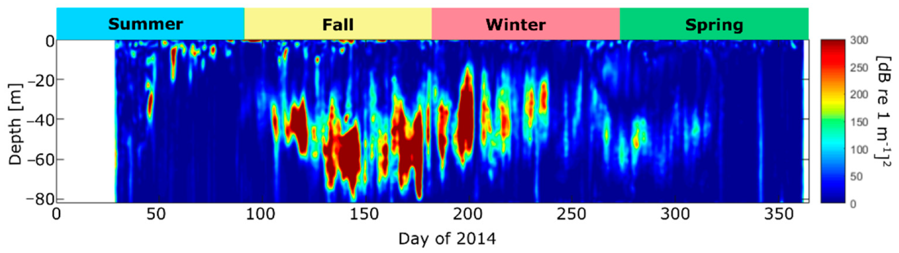
Temperature, salinity, and density profiles from austral fall and spring to summer indicate that during the austral fall, the pycnocline occupies a larger vertical extent in the water column (from ~3–12 m depth) and the fresh, surface layer is thinner than during spring and summer (from surface to ~5 m depth) (see Supplementary Material, Figure S1). Elevated Sv (~>-17 dB re m−1) is apparent as a pycnocline that ranges from the surface down to ~20 m depth (Figure 7a) throughout 2014. The largest values appear in the period 16–22 April (austral Autumn). The depth average of Sv indicates that the austral fall and winter contain the most pronounced diel and intra-monthly variability. However, the Sv values are larger during austral spring and summer than fall (Figure 7b). The increase in Sv during austral summer is attributed to enhanced sediments in the water column due to GLOF 15, which occurred on 1 February 2014 (Figure 7a,c). GLOF 15 resulted in river discharge values exceeding 4000 m3 s−1, a much larger discharge than that of GLOF II in 2010 (~2200 m3 s−1). High-frequency (diel) pulses in Sv were also prominent throughout most of the time series, which are thought to be attributed to diel vertical migrations (DVM) of zooplankton, although if DVMs were taking place during austral summer, the signal appears to be masked by GLOF 15.
In addition to the DVM patterns found in Sv during 2014, there are instances of elevated Sv at the deepest depths that attenuate towards the surface. These pulses are found on approximately days 47, 54, 56, 74, 88, 234, 255, 321, and 342 and show a downward propagation from surface to bottom. They appear to be semidiurnal near the surface and represent sediment cascades from the pycnocline (where sediments are trapped) and subsequently released, accumulating at deeper depths.
3.2.1. Seasonal Changes in Zooplankton
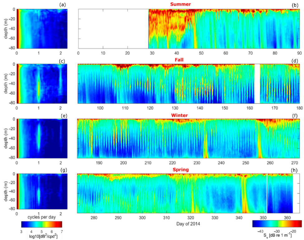
Although in-situ zooplankton samples were not available in 2014, the volume backscatter, Sv, is used as a proxy for zooplankton abundance in the fjord. Sv is separated by season, and a spectral analysis used to determine if a DVM pattern is present, as was done for the 2010 dataset (Figure 5 and Figure 8). As there were more data available during each season of 2014 compared to that of 2010, the spectral signals are better defined (Figure 8). Overall, the spectral analysis shows higher energy at diurnal frequencies than at the semidiurnal tidal frequency, as was found in 2010. The only exception is during austral summer (January–March) when the acoustic signal from GLOF 15 masked both the tidal and DVM signal (Figure 8a,b). High spectral energy at the diel frequency during austral fall, winter and spring is most elevated between ~20–80 m depth, indicating that the DVM does not extend above the pycnocline and is most pronounced below the depth extent of the ADCP moored in 2010. This could be why the spectral energy at 1 cpd during the fall of 2010 (Figure 5a) is weak compared to that of 2014 (Figure 8c).
In order to determine at what depths and times the DVM patterns were the strongest in 2014, a wavelet analysis is carried out at each depth bin of the Sv, and the energy at the diurnal frequency extracted (Figure 9). This analysis shows that the DVM indeed start in the austral fall and extend to the spring, with the intensity of the signal decreasing toward the spring months. During austral fall the DVM extends from ~30 to 80 m depth, while during the winter from ~20 to 60 m depth. During the summer there are only isolated instances of elevated energy at the diurnal frequency (days ~49 and 60), but this could be attributed to the GLOF masking the DVM periodicity.
3.2.2. GLOF 15–1 February 2014
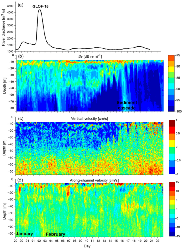
GLOF 15 occurred on 1 February 2014 while the ADCP was moored at ~80 m depth, making it possible to capture the depth influence of the GLOF 15 waters and sediments, which was not captured for GLOF II (Figure 6 and Figure 10). The maximum river discharge from GLOF 15 was 4239 m3 s−1. The discharge pulse over 2000 m3 s−1 (indicative of a GLOF) lasted for 37 h from 1–3 February 2014 (Figure 10a). The Sv data show the highest values at ~10 m depth, indicating that most of the sediment and other particulate organic matter from the GLOF-15 is retained in the pycnocline zone (Figure 10a,b). However, increased Sv related to the GLOF did extend to ~60 m depth. As with GLOF II, Sv became elevated before the maximum flood waters were recorded (29 January–1 February). As was surmised for GLOF II, this response could be due to some flood waters becoming released before the ice dam fully broke. More data are needed in order to verify this hypothesis. The vertical velocity (w) from the ADCP evidenced a consistent settling of the terrestrial-derived sediment (~−1 cm s−1), introduced to the fjord from GLOF 15, from the surface to ~50 m depth from 29 January to 12 February (Figure 10c).
The Sv also revealed two sediment cascade events (5 February and 16 February) where sediments or other materials suspended in the pycnocline descended to the bottom of the fjord (Figure 10b). The sediment cascade events began concurrently with elevated Sv, downward vertical velocities (~1 cm s−1), and enhanced vertical shear in the along-channel flow (u) between ~10–15 m depth (Figure 10b–d). This effect is most pronounced on the 16th of February, when along-channel velocities indicate in-fjord flow at the surface reaching 15 cm s−1 from the surface to ~10 m depth and out-fjord flow below reaching ~−10 cm s−1 from ~10–20 m depth. This reversal in the typical estuarine circulation pattern found in estuaries and fjords (outflow at the surface and inflow at depth) could be a result of in-fjord directed wind enhancing near-surface velocities and will be elaborated upon in the discussion section. In addition, the Sv signal extends further in the water column at this time indicating a deepening of the pycnocline. Therefore, enhanced mixing of the interfacial density layers can allow sediments trapped in the pycnocline to be suddenly released, which can have implications on the nutrients input at depth in the fjord.
4. Discussion
This study investigates how physical properties (currents and pycnocline location) of a glacial fjord in Chilean Patagonia affects zooplankton aggregation in different austral seasons and during GLOF events. Results revealed that zooplankton abundance in the upper water column (surface to ~25 m depth) is most pronounced in austral winter and spring of 2010 from both in-situ zooplankton samples and the volume backscatter, Sv. However, wavelet analysis of Sv during 2014 revealed highest energy at a diurnal frequency (linked to DVM of zooplankton) during the austral fall, but below ~20 m depth, indicating the zooplankton are still present, just located at deeper depths than during austral winter and spring (Figure 9). However, it could also be that the enhanced sediments near the pycnocline mask the energy at the diel frequency as was found during the GLOF. During both 2010 and 2014 the DVM of zooplankton appeared to be limited by the location of the pycnocline, which varied depending on the season and on synoptic time scales.
4.1. Comparison of 2010 and 2014
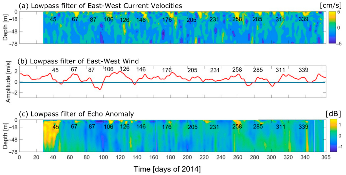
The highest Sv signal was found in late winter and into the spring seasons of 2010 (Figure 5) and in the spring, summer, and fall of 2014 (Figure 8). However, the 2010 dataset did not include measurements from the summer. From mid-August to the end of September of 2010, an increase in the Sv signal near the surface was indicative of a deepening of the pycnocline layer (Figure 5d). The low frequency modulation was the result of wind setup, which created a downward slope of the pycnocline from the fjord mouth toward the head of Martinez Channel, which relaxed upon cessation of the wind [31]. This was found to be a result of the Baroclinic Annular Mode (BAM), which produces periods of enhanced storminess in the extratropical southern hemisphere every 20–30 days [31]. During 2014, this pattern was also found in the volume backscatter and the along-channel current velocities (Figure 11). In fact, throughout the year of 2014 every 19–30 days, near-surface along-channel flows were directed into the estuary, concurrently with up-estuary winds (Figure 11a,b). Further, at almost each instance of up-estuary along-channel flows and wind, the Sv was also elevated. This indicates that the BAM influences the physics of Martinez Channel both intra- and inter-annually, which was unresolved in [31].
The implications of the BAM synoptic events on zooplankton aggregation in Martinez Channel and other fjords in the region is unknown. Zooplankton displacements from/to the continental shelf have been documented in northern hemisphere fjords but were found to be associated with oceanographic processes at seasonal scales [47,48,49] and not with frequencies similar to BAM or associated with the less predictable GLOF events. As the BAM is known only to be a phenomenon of the southern hemisphere, this is not surprising, however it allows a unique opportunity for the biology of southern hemisphere fjords to display periodic, predictable behavior. Gonzalez et al. [50] found that pycnocline depth, nutrient concentration, and seasonal variability in solar radiation are the main factors affecting the extent and timing of primary production in Chilean Patagonia fjords, implying that BAM-induced pycnocline vertical excursions could alter primary production patterns. Moreover, wind-driven surface currents have been found to be responsible for the transport of phytoplankton [51]. For example, Quiroga et al. (2016) [51] found wind driven horizontal advection of phytoplankton in a highly stratified basin. They explain that before the wind ensued, phytoplankton groups were found in layers. However, wind-driven currents mixed the water column and the phytoplankton segregation throughout depth. Further, Meerhoff et al. (2014) [27] studied the advective fluxes of plankton along Martinez Channel. They found that juveniles and adults of multiple plankton and zooplankton species were advected in or out of the fjord depending on whether they were located above or below the pycnocline. Therefore, the synoptic influence on the fjord currents and mixed layer described in this study could alter typical zooplankton abundance and aggregation in Martinez Channel. This effect will only be exacerbated by a GLOF event. However, the high inter-annual variability of environmental conditions should also be considered when comparing the datasets from 2010 and 2014. As was shown in Figure 2, the intensity and frequency of GLOFs are on the rise, indicating that temperatures are also increasing, implying that changes to the fjord dynamics as well as the ecosystem were already underway from 2010 to 2014. Additional years of ADCP data are needed to fully discern the repeatability of zooplankton migration patterns and BAM influence in Martinez Channel.
4.2. Fjord Response to GLOFs
Marin et al. (2013) [13] modeled the effects of GLOFs on the suspended sediment concentration and light availability in the Martinez-Baker fjord complex. Their study suggested that during the GLOF, suspended solids increased 240 times at the head of Martinez Channel due to an influx of glacier particles (or glacial flour). As a result of this increased suspended matter, light extinction was more pronounced near the head of the fjord, extending beyond the junction of Martinez and Steffen Channels (the location of the ADCP mooring for this study). The largest discharge of the Baker River in the hydrographic model study presented by Marin et al. (2013) [13] was 6000 m3 s−1. Although this was higher than the Baker River discharge found in this study (~2200 m3 s−1 in 2010 and ~4200 m3 s−1 in 2014), the effects of the flood were thought to be similar, but on a smaller scale (less surface area affected). The increase in Sv signal during both GLOF II and 15 demonstrated that suspended sediments did indeed increase in Martinez Channel (Figure 4 and Figure 8). This sudden flux of suspended matter was thought to increase light attenuation, which in turn can decrease primary production [27,50]. This is supported by an elevated Sv signal (>-17 dB) during GLOF 15 from 5–10 m depth with a less intense, yet still elevated, signal between 10–60 m depth (>-22 dB, Figure 8a). However, Meerhoff et al., (2019) [25] found that GLOF 15 elevated sediments in the water column, but enhanced productivity due to the elevated nutrients introduced in the system by the glacial flour. In fact, they found an increase in the squat lobster species M. gregaria during the GLOF. When the squat lobster species tissues were sampled, they found that 8% of the sample was composed of terrestrial derived organic carbon from the floodwaters. Therefore, the elevated Sv signal during GLOF 15 was due to enhanced suspended sediments in the water column in addition to increased zooplankton, which implies that the same is likely for GLOF II in 2010.
As addressed in the previous subsection, Martinez Channel showed wind-induced inflow and pycnocline depressions in both 2010 and 2014. During GLOF 15 and shortly thereafter, wind and surface velocities were directed eastward (until day 19 February; Figure 11). The eastward surface flow occurring in conjunction with eastward wind implies that the wind driven flow could retain flood waters near the head of the fjord. Retention of floodwaters could have important implications for local biology as fjords are highly productive ecosystems. The elevated signal in the Sv persisted for ~20 days after the GLOF occurred, indicating that the wind can retain floodwaters and sediment contained within. Sediment retained near the shore could potentially settle in high concentrations and bury marine nurseries rather than dispersing down-fjord, hindering marine populations. In addition, new terrigenous substances introduced by the GLOF, as was found by Meerhoff et al. (2019) [25], could interact with existing organisms in the fjord and influence symbiotic relationships [52].
As there was a synoptic event on days ~30–45 of 2014, enhanced precipitation or storminess (due to the BAM) could have triggered the GLOF event, or at least augmented it. Looking more closely, an enhancement of along-fjord wind occurred on day 45 (15 February, Figure 11), which led to enhanced in-fjord surface currents, and a deepening of the pycnocline. Looking at the Sv, a sediment cascade started on 16 February, caused by a weakening of the interfacial fresh and salt water layer. An investigation into differences between GLOFs occurring during periods of wind-forcing versus periods of wind dormancy would be beneficial as the BAM and GLOFs are both influential phenomena occurring in Martinez Channel. However, the sediment cascades appear to be occurring throughout the time series and not only as a result of the GLOF.
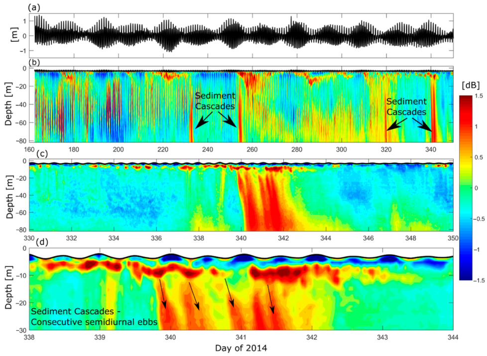
To investigate the occurrence of the sediment cascades and how they correlate to the tide, the echo anomaly and water levels were compared from day 160 to 350 of 2014, when water level measurements were available from the pressure sensor of the ADCP (Figure 12). Sediment cascades are shown on days 232, 255, 320, and 341 (Figure 12b). Focusing on the sediment cascade on day 341, it is apparent that this occurs after a BAM event (Figure 11) when there is elevated near-surface eastward (up-fjord) currents. This implies that the cascades develop after up-fjord winds decrease the discharge from the river by retaining flood waters and the sediments therein. After the wind relaxes, the river sediments are released to the fjord, causing a cascade in consecutive semidiurnal ebbs (Figure 12c,d). The sediments from consecutive ebbs eventually merge at depths between ~20–35 m and accumulate at greater depths. As this is toward the head of the fjord, this could be one of the potential causes of channelized sediment waves found in this fjord [53].
4.3. Zooplankton Detection Using Acoustic Devices during GLOFs
It has been found that high turbidity at the surface of Martinez Channel reduces the need for some zooplankton groups to migrate vertically to avoid predation [27], which is likely why DVM patterns within the fjord were minimal compared to other fjords in the region, e.g., Reloncavi fjord [29]. However, DVM patterns were found both before and after the GLOF II event in 2010, yet were obscured during the event itself (Figure 6). It was unclear whether GLOF II ceased the vertical migrations of zooplankton or whether the increase of glacial flour in the fjord masked the migration signal by reducing light penetration into the water column.
GLOFs have been found to influence the abundance and composition of biology in fjords [27]. High concentrations of suspended sediments have been shown to decrease primary production [22,27], subsequently decreasing secondary production (i.e., zooplankton). This indicates that suspended sediments influxed by a GLOF might decrease DVM of zooplankton by eliminating their food source, phytoplankton. GLOF 15 (in 2014) occurred during mid-to-late summer when primary producer concentrations are typically limited [54]. Consequently, zooplankton have less reason to migrate vertically during this time as food is not as readily available and surface temperatures are higher [27,29]. Therefore, there was no DVM pattern present during the GLOF and there was a decreased DVM pattern after 14 November 2014, as this is when surface temperatures begin warming (Figure S1) and primary production decreases. This is evident from a lack of the high frequency pulses in volume backscatter from 14 November to 1 April (Figure 7 and Figure 8). Although in-situ zooplankton samples during the GLOF events would be helpful in determining if this was indeed the case, it is both unlikely to be in the fjord sampling during a GLOF event due to its unpredictability and dangerous to be on the water during an actual event [55]. Having an acoustic device of multiple frequencies could have helped discern if the volume backscatter signal was zooplankton or sediments and is recommended for future studies.
5. Conclusions
Wind events caused by the southern hemisphere baroclinic annular mode (BAM) in Martinez Channel, Chilean Patagonia were found to regularly (every ~20–30 day) produce up-fjord surface currents and a vertical excursion of the pycnocline. One such event in 2014 took place several days after a glacial lake outburst flood (GLOF) and produced a sediment cascade by weakening the density interface that kept glacial sediments near surface. Further, the wind events produce a periodic deepening of the pycnocline due to the BAM that limited the vertical migrations of zooplankton in the fjord during several austral seasons. This study indicates that the BAM influences Martinez Channel inter- and intra-annually representing a novel finding for this region and suggesting that the BAM could affect the physics and biology in other Patagonian fjords. Considering that South America can be expected to experience an increase in GLOF events, understanding the interaction between the BAM and GLOFs should be emphasized in future studies. Both of these phenomenon can have major implications for local marine life as GLOFs contribute suspended sediment into fjord systems.
Supplementary Materials
The following are available online at https://www.mdpi.com/2073-4441/12/1/248/s1.
Author Contributions
Conceptualization, L.R., I.P.-S., L.C., and A.V.-L.; methodology, L.R., I.P.-S., L.C., and W.S.; formal analysis, L.R., I.P.-S., B.P., and L.C.; investigation, L.R., I.P.-S., L.C., A.V.-L., and W.S.; resources, I.P.-S., L.C., and W.S.; data curation, L.R., I.P.-S., B.P., and L.C.; writing—original draft preparation, L.R., I.P.-S., B.P., L.C., A.V.-L., and W.S.; writing—review and editing, L.R., I.P.-S., B.P., L.C., A.V.-L., and W.S.; project administration, I.P.-S., L.C., and W.S.; funding acquisition, I.P.-S., L.C., and W.S. All authors have read and agreed to the published version of the manuscript.
Funding
This work was funded by CONICYT FONDAP-COPAS Grant 15010007, CONICYT FONDECYT Grant 11140161 and COPAS SUR-AUSTRAL Grant PFB-31/2007 and AFB 170006.
Acknowledgments
We are grateful to Chile’s general water department for providing the Baker River discharge data. We also thank Raúl Montoya and Rodrigo Mansilla for their assistance in the ADCP mooring and Rodrigo Mansilla for conducting most of the zooplankton sampling during the year.
Conflicts of Interest
The authors declare no conflict of interest.
References
- Chen, Y.; Xu, C.; Chen, Y.; Li, W.; Liu, J. Response of glacial-lake outburst floods to climate change in the Yarkant River basin on northern slope of Karakoram Mountains, China. Quat. Int. 2010, 226, 75–81. [Google Scholar] [CrossRef]
- Glick, D. Photograph by Warne, K. Sea Level Rise National Geographic. Available online: www.nationalgeographic.com/environment/global-warming/sea-level-rise/ (accessed on 7 April 2017).
- Harrison, S.; Glasser, N.; Winchester, V.; Haresign, E.; Warren, C.; Jansson, K. A Glacial Lake Outburst Flood Associated with Recent Mountain Glacier Retreat, Patagonian Andes. Holocene 2006, 16, 611–620. [Google Scholar] [CrossRef]
- Somos-Valenzuela, M.A.; Chisolm, R.E.; Rivas, D.S.; Portocarrero, C.; Mckinney, D.C. Modeling a glacial lake outburst flood process chain: The case of Lake Palcacocha and Huaraz, Peru. Hydrol. Earth Syst. Sci. 2016, 20, 2519–2543. [Google Scholar] [CrossRef]
- IPCC. Chapter 4: Sea Level Rise and Implications for Low Lying Islands, Coasts and Communities IPCC SR Ocean and Crosphere; Abe-Ouchi, A., Gupta, K., Periera, J., Eds.; IPCC: Geneva, Switzerland, 2019; pp. 3–11. [Google Scholar]
- Rivera, A.; Benham, T.; Casassa, G.; Bamber, J.; Dowdeswell, A.J. Ice elevation and areal changes of glaciers from the Northern Patagonia Icefield, Chile. Glob. Planet. Chang. 2007, 59, 126–137. [Google Scholar] [CrossRef]
- Valle-Levinson, A. Definition and Classification of Estuaries. In Contemporary Issues in Estuarine Physics; Cambridge University Press: Cambridge, UK, 2010. [Google Scholar] [CrossRef]
- Dyer, K.R. Estuaries: A Physical Introduction, 2nd ed.; John Wiley & Sons: Hoboken, NJ, USA, 1997. [Google Scholar]
- Farmer, D.M.; Freeland, H.J. The physical oceanography of fjords. Prog. Oceanogr. 1983, 12, 147–220. [Google Scholar] [CrossRef]
- Inall, M.E.; Gillibrand, P.A. The physics of mid-Latitude fjords: A review. Fjord Syst. Arch. 2010, 344, 17–33. [Google Scholar] [CrossRef]
- Pantoja, S.; Iriarte, J.L.; Daneri, G. Oceanography of the Chilean Patagonia. Cont. Shelf Res. 2011, 31, 149–153. [Google Scholar] [CrossRef]
- Aiken, C.M. Seasonal thermal structure and exchange in Baker Channel, Chile. Dyn. Atmos. Ocean. 2012, 58, 1–19. [Google Scholar] [CrossRef]
- Marín, V.H.; Tironi, A.; Parades, M.A.; Contreras, M. Modeling suspended solids in a Northern Chilean Patagonia glacier-Fed fjord: GLOF scenarios under climate change conditions. Ecol. Model. 2013, 264, 7–16. [Google Scholar] [CrossRef]
- Dussaillant, A.; Benito, G.; Buytaert, W.; Carling, P.; Meier, C.; Espinoza, F. Repeated glacial-lake outburst floods in Patagonia: An increasing hazard? Nat. Hazards 2009, 54, 469–481. [Google Scholar] [CrossRef] [Green Version]
- Palmer, J. Chiles glacial lakes pose newly recognized flood threat. Science 2017, 355, 1004–1005. [Google Scholar] [CrossRef] [PubMed]
- Kattelmann, R. Glacial Lake Outburst Floods in the Nepal Himalaya: A manageable Hazard? Nat. Hazards 2003, 28, 145–154. [Google Scholar] [CrossRef]
- Breien, H.; De Blasio, F.V.; Elverhoi, A.; Hoeg, K. Erosion and morphology of a debris flow caused by a glacial lake outburst flood, Western Norway. Landslides 2008, 5, 271–280. [Google Scholar] [CrossRef]
- Cook, S.J.; Kougkoulos, I.; Edwards, L.A.; Dortch, J.; Hoffmann, D. Glacier change and glacial lake outburst flood risk in the Bolivian Andes. Cryosphere 2016, 10, 2399–2413. [Google Scholar] [CrossRef] [Green Version]
- Margold, M.; Jansson, K.N.; Stroeven, A.P.; Jansen, J.D. Glacial Lake Vitim, a 3000-km3 outburst flood from Siberia to the Arctic Ocean. Quat. Res. 2011, 76, 393–396. [Google Scholar] [CrossRef]
- Lopez, P.; Chevallier, P.; Favier, V.; Pouyaud, B.; Ordenes, F.; Oerlemans, J. A regional view of fluctuations in glacier length in southern South America, Glob. Planet. Chang. 2010, 71, 85–108. [Google Scholar] [CrossRef]
- Casassa, G.; Wendt, J.; Wendt, A.; Lopez, P.; Schuler, T.; Maas, H.; Carrasco, J.; Rivera, A. Outburst floods of glacial lakes in Patagonia: Is there an increasing trend? Geophys. Res. Abstr. 2010, 12, 12821. [Google Scholar]
- Montecino, V.; Pizarro, G.; Baker, C.; Fallos, C. Primary productivity, biomass, and phytoplankton size in the austral Chilean channels and fjords: Spring–summer patterns. In Progress in the Oceanographic Knowledge of Chilean Interior Water; Comité Oceanográfico Nacional-Pontificia Universidad Católica de Valparaíso: Valpariso, Chile, 2008; pp. 93–97. [Google Scholar]
- Pizarro, G.; Montecinos, V.; Guzmán, L.; Chacón, V.; Pacheco, H.; Frangópolus, M.; Retamal, L.; Alarcón, C. Recurrent local patterns of phytoplankton in fjords and channels (43–56° S) during austral spring and summer. Cienc. Tecnol. 2005, 28, 63–83. [Google Scholar]
- Aracena, C.; Lange, C.B.; Iriarte, J.L.; Rebolledo, L.; Pantoja, S. Latitudinal patterns of export production recorded in surface sediments of the Chilean Patagonian fjords (41–55° S) as a response to water column productivity. Cont. Shelf Res. 2011, 31, 340–355. [Google Scholar] [CrossRef]
- Meerhoff, E.; Castro, L.R.; Tapia, F.J.; Perez-Santos, I. Hydrographic and biological impacts of a Glacial Lake Outburst Flood (GLOF) in a Patagonian Fjord. Estuaries Coasts 2019. [Google Scholar] [CrossRef]
- Klevjer, T.A.; Irigoien, X.; Rostad, A.; Fraile-Nuez, E.; Benitez-Barrios, V.M.; Kaartvedt, S. Large scale patterns in vertical distribution and behavior of mesopelagic scattering layers. Sci. Rep. 2016, 6. [Google Scholar] [CrossRef] [Green Version]
- Meerhoff, E.; Tapia, F.J.; Sobarzo, M.; Castro, L.R. Influence of estuarine and secondary circulation on crustacean larval fluxes: A case study from a Patagonian fjord. J. Plankton Res. 2014, 37, 168–182. [Google Scholar] [CrossRef] [Green Version]
- Alldredge, A.L.; King, J.M. Effects of moonlight on the vertical migration patterns of demersal zooplankton. J. Exp. Mar. Biol. Ecol. 1980, 44, 133–156. [Google Scholar] [CrossRef]
- Valle-Levinson, A.; Castro, L.; Cáceres, M.A.; Pizarro, O. Twilight vertical migrations of zooplankton in a Chilean fjord. Prog. Oceanogr. 2014, 129, 114–124. [Google Scholar] [CrossRef]
- Piret, L.; Bertrand, S.; Vandekerkhove, E.; Harada, N.; Moffat, C.; Rivera, A. Gridded Bathymetry of the Baker-Martinez Fjord Complex (Chile, 48° S) v1. Available online: https://figshare.com/articles/Gridded_bathymetry_of_the_Baker-Martinez_fjord_complex_Chile_48_S_v1/5285521 (accessed on 9 September 2017).
- Ross, L.; Valle-Levinson, A.; Pérez-Santos, I.; Tapia, F.J.; Schneider, W. Baroclinic annular variability of internal motions in a Patagonian fjord. J. Geophys. Res. Ocean. 2015, 120, 5668–5685. [Google Scholar] [CrossRef] [Green Version]
- Ross, L.; Pérez-Santos, I.; Valle-Levinson, A.; Schneider, W. Semidiurnal internal tides in a Patagonian fjord. Prog. Oceanogr. 2014, 129, 19–34. [Google Scholar] [CrossRef]
- Thompson, D.W.J.; Barnes, E.A. Periodic variability in the large-scale southern hemisphere atmospheric circulation. Science 2014, 343, 641–645. [Google Scholar] [CrossRef]
- Thompson, D.W.J.; Woodworth, J.D. Barotropic and baroclinic annular variability in the southern hemisphere. J. Atmos. Sci. 2014, 71, 1480–1493. [Google Scholar] [CrossRef]
- Pérez-Santos, I.; Seguel, R.; Schneider, W.; Linford, P.; Donoso, D.; Navarro, E.; Amaya-Carcamo, C.; Pinilla, E.; Daneri, G. Synoptic-scale variability of surface winds and ocean response to atmospheric forcing in the eastern austral Pacific Ocean. Ocean Sci. 2019, 15, 1247–1266. [Google Scholar] [CrossRef] [Green Version]
- Meerhoff, E.; Tapia, F.J.; Castro, L.R. Spatial structure of the meroplankton community along a Patagonian fjord—The role of changing freshwater inputs. Prog. Oceanogr. 2014, 129, 125–135. [Google Scholar] [CrossRef]
- Castro, L.R.; Troncoso, V.A.; Figueroa, D.R. Fine-scale vertical distribution of coastal and offshore copepods in the Golfo de Arauco, central Chile, during the upwelling season. Prog. Oceanogr. 2007, 75, 486–500. [Google Scholar] [CrossRef]
- Castro, L.R.; Caceres, M.A.; Silva, N.; Munoz, M.I.; Leon, R.; Landaeta, M.F.; Soto-Mendoza, S. Short-term variations in mesozooplankton, icthyoplankton, and nutrients associated with semi-diurnal tides in Patagonian Gulf. Cont. Shelf Res. 2011, 31, 282–292. [Google Scholar] [CrossRef]
- Valle-Levinson, A.; Trasviña-Castro, A.; de Velasco, G.G.; Armas, R.G. Diurnal vertical motions over a seamount of the southern Gulf of California. J. Mar. Syst. 2004, 50, 61–77. [Google Scholar] [CrossRef]
- Rippeth, T.P.; Simpson, J.H. Diurnal signals in vertical motions on the Hebridean Shelf. Limnol. Oceanogr. 1998, 43, 1690–1696. [Google Scholar] [CrossRef]
- Greene, C.H.; Wiebe, P.H. Bioacoustical oceanography: New tools for zooplankton and micronekton research in the 1990s. Oceanography 1990, 3, 12–17. [Google Scholar] [CrossRef] [Green Version]
- Brierley, A.S.; Saunders, R.A.; Bone, D.G.; Murphy, E.J.; Enderlein, P.; Conti, S.G.; Demer, D.A. Use of moored acoustic instruments to measure short-term variability in abundance of Antarctic krill, Limnology and Oceanography. Methods 2006, 4, 18–29. [Google Scholar]
- Lee, K.; Mukai, T.; Kang, D.H.; Iida, K. Application of acoustic Doppler current profiler combined with a scientific echo sounder for krill Euphausia pacifica density estimation. Fish. Sci. 2004, 70, 1051–1060. [Google Scholar] [CrossRef]
- Wiebe, P.H.; Mountain, D.; Stanton, T.K.; Greene, C.H.; Lough, G.; Kaartvedt, S.; Dawson, J.; Coply, N. Acoustical studies of the spatial distribution of plankton on Georges Bank and the relationship between volume backscattering strength and the taxonomic composition of plankton. Deep Sea Res. II 1996, 43, 1971–2001. [Google Scholar] [CrossRef]
- Emery, W.J.; Thomson, R.E. Data Analysis Methods in Physical Oceanography, 2nd ed.; Elsevier: Amsterdam, The Netherlands, 2004; pp. 319–325. [Google Scholar]
- Torrence, C.; Compo, G.P. A practical guide to wavelet analysis. Bull. Am. Meteorol. Soc. 1998, 79, 61–78. [Google Scholar] [CrossRef] [Green Version]
- Walkusz, W.; Kwasniewski, S.; Falk-Petersen, S.; Hop, H.; Tverberg, V.; Wieczorek, P.; Weslawski, J.M. Seasonal and spatial changes in the zooplankton community of Kongsfjorden, Svalbard. Polar Res. 2009, 28, 254–281. [Google Scholar] [CrossRef]
- Gluchowska, M.; Kwasniewski, S.; Prominska, A.; Olszewska, A.; Goszczko, I.; Falk-Peterson, S.; Hop, H.; Weslawski, J.M. Zooplankton in Svalbard fjords on the Atlantic-Arctic boundary. Polar Biol. 2016, 39, 1785–1802. [Google Scholar] [CrossRef] [Green Version]
- Ormanczyk, M.R.; Gluchowska, M.; Olszewska, A.; Kwasniewski, S. Zooplankton structure in high latitude fjords with contrasting oceanography (Hornsund and Kongsfjorden, Spitsbergen). Oceanologia 2017, 59, 508–524. [Google Scholar] [CrossRef]
- Gonzalez, H.E.; Castro, L.; Daneri, G.; Iriarte, J.L.; Silva, N.; Vargas, C.; Giesecke, N.; Sanchez, N. Seasonal plankton variability in Chilean Patagonia Fjords: Carbon flow through the pelagic food web of the Aysen Fjord and plankton dynamics in the Moraleda Channel basin. Cont. Shelf Res. 2011, 31. [Google Scholar] [CrossRef]
- Quiroga, E.; Ortiz, P.; Gonzalez-Saldias Reid, B.; Tapia, F.J.; Perez-Santos, I.; Rebolledo, L.; Mansilla, R.; Pineda, C.; Cari, I.; Salinas, N.; et al. Seasonal benthic patterns in a glacial Patagonian fjord: The role of suspended sediment and terrestrial organic matter. Mar. Ecol. Prog. Ser. 2016, 561, 31–50. [Google Scholar] [CrossRef]
- Serra, T.; Vidal, J.; Colomer, J.; Casamitjana, X.; Soler, M. The role of surface vertical mixing in phytoplankton distribution in a stratified reservoir. Limnol. Oceanogr. 2007, 52, 620–634. [Google Scholar] [CrossRef] [Green Version]
- Vandekerkhove, E.; Bertrand, S.; Lanna, E.C.; Reid, B.; Pantoja, S. Modern sedimentary processes at the heads of Marinez Channel and Steffen Fjord, Chilean Patagonia. Mar. Geol. 2019. [Google Scholar] [CrossRef]
- Meire, L.; Mortenson, J.; Meire, P.; Juul-Pedersen, T.; Sejr, M.K.; Rysgaard, S.; Nygaard, R.; Huybrechts, P.; Meysmen, F.J.R. Marine-terminating glaciers sustain high productivity in Greenland fjords. Glob. Chang. Biol. 2017. [Google Scholar] [CrossRef] [PubMed]
- Carey, M. Living and dying with glaciers: people’s historical vulnerability to avalanches and outburst floods in Peru. Glob. Planet. Chang. 2005, 47, 122–134. [Google Scholar] [CrossRef]
Figure 1.
(a) Study area in relation to South America. (b) Close up of study area identifying the Northern and Southern Patagonia Icefields. (c) Further close up identifying the Acoustic Doppler Current Profiler (ADCP) mooring and Conductivity, Temperature, Depth (CTD) station location within Martinez Channel, the Baker River, the location where river discharge measurements were collected (DGA stations) and Lake Cachet-2, where the glacial lake outburst floods (GLOFs) begin. These figures were modified from data available by the National Oceanic and Atmospheric Administration (NOAA) Bathymetry Viewer.

Figure 2.
(a) Time series of Baker river discharge at the DGA Ñadis station from 2003–2014. The red dots denote the GLOF events reported by the DGA and blue dots represent other possible GLOF events. (b) Long-term monthly mean river discharge with the standard deviations.
Figure 2.
(a) Time series of Baker river discharge at the DGA Ñadis station from 2003–2014. The red dots denote the GLOF events reported by the DGA and blue dots represent other possible GLOF events. (b) Long-term monthly mean river discharge with the standard deviations.

Figure 3.
(a) Volume backscattering strength (Sv, in dB re 1 m−1) from autumn to spring of 2010. (b) The depth average of Sv in black with the 30 h low-passed time series depicted by the center line. (c) Hourly Baker River discharge measurements (m3 s−1).
Figure 3.
(a) Volume backscattering strength (Sv, in dB re 1 m−1) from autumn to spring of 2010. (b) The depth average of Sv in black with the 30 h low-passed time series depicted by the center line. (c) Hourly Baker River discharge measurements (m3 s−1).

Figure 4.
(a) Quantity of copepods from 25 m depth to the surface collected during monthly in-situ zooplankton samples throughout the year of 2010. (b) Same as (a) but for all other zooplankton species found in the samples.
Figure 4.
(a) Quantity of copepods from 25 m depth to the surface collected during monthly in-situ zooplankton samples throughout the year of 2010. (b) Same as (a) but for all other zooplankton species found in the samples.

Figure 5.
(a) Spectra of the autumn time series of Sv (log10 (dB2/cpd2)), (b) is the autumn Sv time series. (c,d) are the same as (a,b) for the winter time series. (e,f) are the same as (a,b) for the spring time series. (g) Time averages of Sv for each season.
Figure 5.
(a) Spectra of the autumn time series of Sv (log10 (dB2/cpd2)), (b) is the autumn Sv time series. (c,d) are the same as (a,b) for the winter time series. (e,f) are the same as (a,b) for the spring time series. (g) Time averages of Sv for each season.

Figure 6.
(a) Sv during the GLOF II event. (b) Baker River discharge values and temperature measurements collected at the same location as river discharge measurements (°C). (c) Vectors of the horizontal velocity components collected from the ADCP (cm s−1) at 5 m depth. (d) Same as (c) for 15 m depth. (e) Temperature measured from the ADCP (°C) at 30 m depth. (f) Squared vertical shear (log10(s−2)).

Figure 7.
(a) Volume backscatter, Sv from January to December of 2014, (b) the depth average of Sv (black line) and the low-pass filtered (30 h), depth-averaged Sv (red line), (c) river discharge (black line) with a discharge value of 2000 m3 s−1, indicative of a GLOF, depicted by the red line.
Figure 7.
(a) Volume backscatter, Sv from January to December of 2014, (b) the depth average of Sv (black line) and the low-pass filtered (30 h), depth-averaged Sv (red line), (c) river discharge (black line) with a discharge value of 2000 m3 s−1, indicative of a GLOF, depicted by the red line.

Figure 8.
(a) Spectra of Sv from the austral summer (January–March) at each depth (y-axis), (b) time series of Sv from the austral summer. (c,d) are the same as (a,b) but for the austral fall (April–June), (e,f) are the same as (a,b) but for the austral winter (July–September), (g,h) are the same as (a,b) but for austral spring (October–December).

Figure 9.
Wavelet analysis of the diurnal frequency of Sv at each depth bin for the entire 2014 time series.
Figure 9.
Wavelet analysis of the diurnal frequency of Sv at each depth bin for the entire 2014 time series.

Figure 10.
(a) Hourly measurements of river discharge at Ñadis station showing the GLOF-15 event occurrence on 1 February 2014, (b) volume backscatter, Sv indicating the occurrence of the sediment cascade (16 February) (c) vertical velocity, w and (d) along-channel velocity, u where positive values denote in-fjord flow and negative values denote out-fjord flow.

Figure 11.
(a) Low-pass filtered (5 day) east-west (along-channel) velocities where the numbers indicate a day of 2014 when the low-passed currents were sustained above 5 cm s−1 for over a 5 day period. (b) Low-pass filtered east-west wind with the same days marked as in (a), and (c) low-pass filtered echo anomaly.

Figure 12.
(a) Water level (m), (b) echo anomaly from day 160 to 350 of 2014 showing times of sediment cascades, (c) zoom in from day 330 to 350 of 2014 showing the sediment cascade from day 340 to 343 of 2014, (d) further zoom of sediment cascade from day 338 to 344 showing the sediment cascades taking place on consecutive semidiurnal ebb tides.


Table 1.
GLOF events reported and validated by the Chilean Water Directorate.
| GLOF Number | Date dd Month yyyy | Austral Season |
|---|---|---|
| 1 | 6 April 2008 | Fall |
| 2 | 10 July 2008 | Spring |
| 3 | 21 December 2008 | Spring |
| 4 | 04 March 2009 | Summer |
| 5 | 16 September 2009 | Winter |
| 6 | 05 January 2010 | Summer |
| 7 | 04 March 2011 | Summer |
| 8 | 29 May 2011 | Fall |
| 9 | 26 January 2012 | Summer |
| 10 | 01 April 2012 | Fall |
| 11 | 07 November 2012 | Spring |
| 12 | 08 February 2013 | Summer |
| 13 | 10 April 2013 | Fall |
| 14 | 23 September 2013 | Spring |
| 15 | 01 February 2014 | Summer |
| 16 | 17 August 2014 | Winter |
| Other Possible Events | ||
| I | 02 May 2010 | Fall |
| II | 29 June 2010 | Fall |
| III | 12 October 2010 | Spring |
© 2020 by the authors. Licensee MDPI, Basel, Switzerland. This article is an open access article distributed under the terms and conditions of the Creative Commons Attribution (CC BY) license (http://creativecommons.org/licenses/by/4.0/).
Share and Cite
MDPI and ACS Style
Ross, L.; Pérez-Santos, I.; Parady, B.; Castro, L.; Valle-Levinson, A.; Schneider, W. Glacial Lake Outburst Flood (GLOF) Events and Water Response in A Patagonian Fjord. Water 2020, 12, 248. https://doi.org/10.3390/w12010248
AMA Style
Ross L, Pérez-Santos I, Parady B, Castro L, Valle-Levinson A, Schneider W. Glacial Lake Outburst Flood (GLOF) Events and Water Response in A Patagonian Fjord. Water. 2020; 12(1):248. https://doi.org/10.3390/w12010248
Chicago/Turabian StyleRoss, Lauren, Iván Pérez-Santos, Brigitte Parady, Leonardo Castro, Arnoldo Valle-Levinson, and Wolfgang Schneider. 2020. "Glacial Lake Outburst Flood (GLOF) Events and Water Response in A Patagonian Fjord" Water 12, no. 1: 248. https://doi.org/10.3390/w12010248
Note that from the first issue of 2016, this journal uses article numbers instead of page numbers. See further details here.