Multi-Objective Optimization for Selecting and Siting the Cost-Effective BMPs by Coupling Revised GWLF Model and NSGAII Algorithm

Abstract

Best management practices (BMPs) are an effective way to control water pollution. However, identification of the optimal distribution and cost-effect of BMPs provides a great challenge for watershed policy makers. In this paper, a semi-distributed, low-data, and robust watershed model, the Revised Generalized Watershed Loading Function (RGWLF), is improved by adding the pollutant attenuation process in the river channel and a bank filter strips reduction function. Three types of pollution control measures—point source wastewater treatment, bank filter strips, and converting farmland to forest—are considered, and the cost of each measure is determined. Furthermore, the RGWLF watershed model is coupled with a widely recognized multi-objective optimization algorithm, the non-dominated sorting genetic algorithm II (NSGAII), the combination of which is applied in the Luanhe watershed to search for spatial BMPs for dissolved nitrogen (DisN). Fifty scenarios were finally selected from numerous possibilities and the results indicate that, at a minimum cost of 9.09 × 10⁷ yuan, the DisN load is 3.1 × 10⁷ kg and, at a maximum cost of 1.77 × 10⁸ yuan, the total dissolved nitrogen load is 1.31 × 10⁷ kg; with the no-measures scenario, the DisN load is 4.05 × 10⁷ kg. This BMP optimization model system could assist decision-makers in determining a scientifically comprehensive plan to realize cost-effective goals for the watershed.

1. Introduction

Water pollution has received increasing attention, and many countries have increased their investments into water pollution control and water resources protection [1]. Designing scientific, reasonable, and efficient management measures to control or reduce pollutants at the watershed scale has become one of the most challenging problems for policy researchers and decision makers [2]. Many policies for the selection of best management practice (BMPs) have been created and applied to specific cases all around the world. For example, the United States and Europe have developed the corresponding Total Maximum Daily Loads and European Water Framework Directive for such purposes [3,4]. The implementation of these plans has provided a sufficient theoretical basis for subsequent watershed governance research [5].

BMPs are the most effective measure for controlling watershed pollution, including vegetative filter strips, land-use transformation, reducing the amount of fertilizer, terraces, and so on [6]. In general, BMP implementation plans should consist of a combination of maximum pollution reduction and minimal financial costs, due to limited budgets [7]. To our best knowledge, there are three optimization techniques which achieve the purpose. The first is setting a fixed number of scenarios manually and then calculating the corresponding pollutant production and cost separately [8,9]. By comparing the results of a limited number of different BMP scenarios, the final solution can be picked out. This method is straightforward and easy to implement, but may cause biased results as it depends on the experience of managers. Thus, the solution may not be the most cost-effective at the watershed scale [10]. The second is aggregating the environmental goals and economic factors into a single compromised objective function (e.g., a genetic algorithm or TaBu search algorithm) [11,12]. Through coupling the watershed model and optimization algorithm, only one optimal solution can be searched [13]. Compared with the first method, this method is more objective but usually takes more time, due to the necessary model runtime for each population per generation. The last technique is the coupling of a multi-objective optimization algorithm and a distributed watershed model to search over a set of solutions. This technique is similar to the second one, but it is able to provide a range of different trade-off BMPs among two or more conflicting objective functions. Due to its comprehensiveness and accuracy, it has been widely used in recent years [14].

The non-dominated sorting genetic algorithms II (NSGAII) is the most popular method for multi-objective optimization, whose ultimate goal is to find “Pareto-optimal” solutions, which is a modified version based on the genetic algorithm [15]. For example: Maringanti et al. utilized the Soil and Water Assessment Tool (SWAT) model and NGSAII to analyze the funding input under different combinations of fertilization reduction ratios, riparian filter belt widths, and other agricultural management measures in a tributary of the Mississippi River [16,17]; Ahmadi et al. combined the SWAT model and the NSGAII algorithm to evaluate the prevention and treatment effects of Atrazine through various evaluation indicators and non-point source management measures in the Eagle Creek Watershed in Indiana, USA [18]; and Geng et al. coupled the SWAT model and NSGAII algorithm to calculate the relationship between the amount of nutrient reduction and the required funding in the Chaohe River Watershed upstream of the Miyun Reservoir in China [19]. However, almost all studies in this category have focused on non-point source pollution BMPs and ignored point source BMP measures. It can be inferred, therefore, that the description of point source measures is not easy in the management practices of the watershed model.

Besides the selection of optimization technique, effective watershed management requires an understanding of the fundamental hydrologic and physicochemical processes in the watershed system, which are non-linear, dynamical, and complex [20]. Therefore, the applicability of the basin watershed model is very essential. A number of comprehensive watershed models have been developed to simulate hydrology and water quality in basins, and previous studies have demonstrated that some watershed models are well-behaved for the selection and targeted placement of BMPs (e.g., SWAT and AnnAGNPS) [21,22]. However, the watershed models in most previous studies have a high demand for data, and are difficult to apply in some areas where there is a lack of data [23]. The Revised Generalized Watershed Loading Function (RGWLF) is an improved semi-distributed hydrological model based on the Generalized Watershed Loading Function (GWLF) model, which has favorable stability, robustness, and less data requirements [24].

Given the above considerations, in this study, we incorporated RGWLF and NSGAII to identify a set of optimal BMPs based on both point and non-point source pollution control practices. Three tasks were completed to accomplish this research target: (1) adding the nutrient channel routing algorithms into the RGWLF then calibrating and verifying the parameters of the model; (2) determining the specific point source and non-point source management measures based on the established model; and (3) coupling the RGWLF model and NSGAII optimization algorithm based on a parameter sensitivity analysis to identify the optimal spatial allocation of BMPs for dissolved nitrogen.

2. Materials and Methods

2.1. Study Area and Data Sources

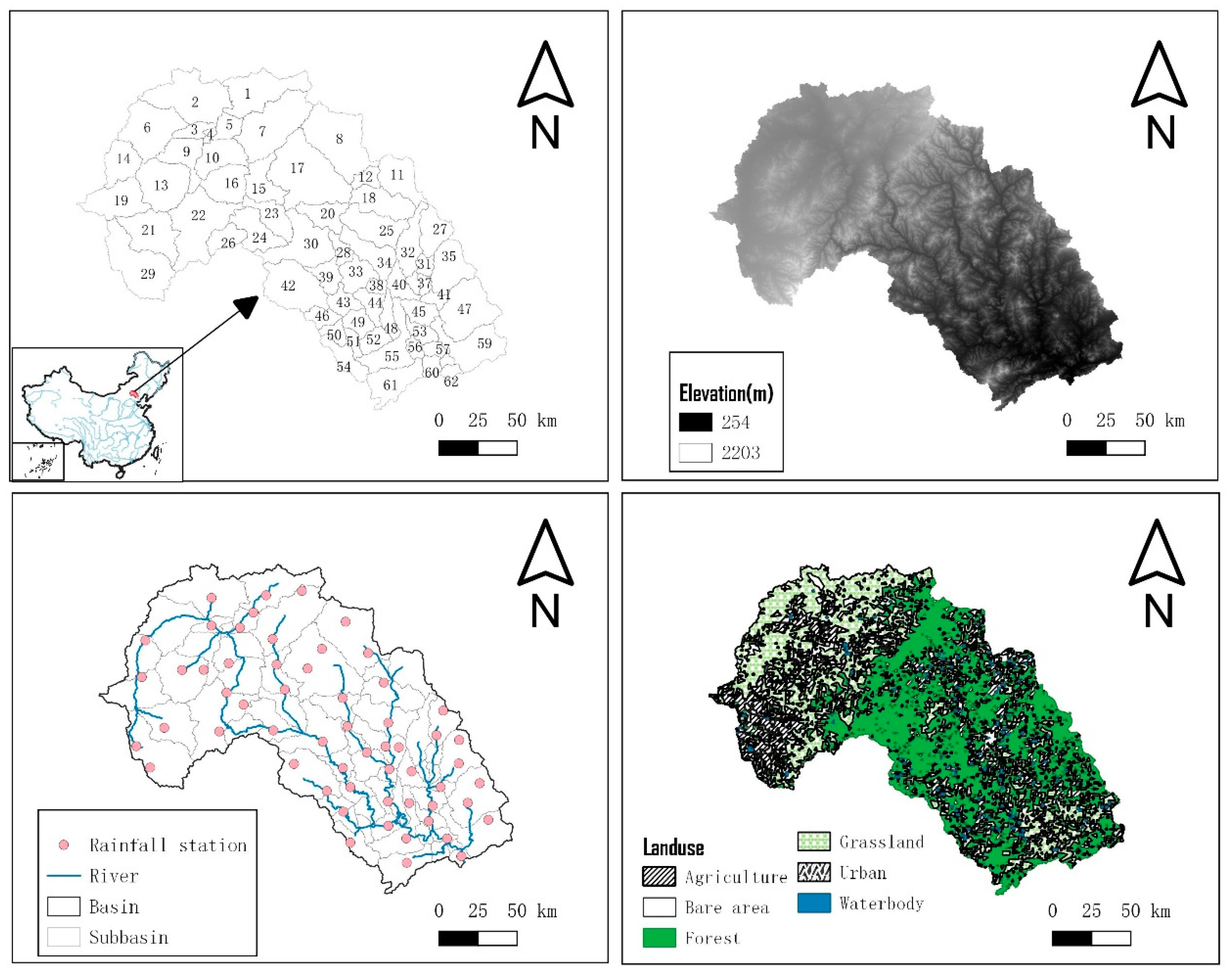
The Luanhe River watershed, which is located in North China (Figure 1), was selected in this study. It is a major component of one of the nine main river watersheds in China: the Haihe River watershed. It has been listed by the Chinese government as an important ecological conservation area in the Beijing–Tianjin–Hebei region. At the same time, its downstream reservoir is an important source of drinking water. The study watershed covers an area of about 30,000 km². According to the 2010 national Land Cover Data set, the watershed consists of 39.2% forest, 33.3% grassland, 21.6% agricultural area, and 1% water bodies. The climate is dominated by temperate semiarid monsoon climate. From 2000–2014, the annual average temperature for this area was 5.7 °C and the mean annual precipitation was 422 mm. Most of the precipitation was concentrated between April and August.

QGIS3 (https://qgis.org/en/site/index.html) and TauDEM (http://hydrology.usu.edu/taudem) were used to divide the Luanhe River Watershed into 62 sub-basins. Climate data were obtained from the Annual Hydrological Report P. R. China for precipitation data and the China Meteorological Data Service Center for temperature data. Thirty-meter resolution digital elevation models (DEMs) were downloaded from the Geospatial Data Cloud (http://www.gscloud.cn). Furthermore, a land-use map (in vector format) was provided by the National Earth System Science Data Center (http://www.geodata.cn). Observed flow data were gathered from the Annual Hydrological Report P. R. China. The hydrological monitoring station and the water quality monitoring station are located in sub-basin 62, which is at the outlet of the whole watershed. The above-mentioned data for the model setup are summarized in

Table 1. Watershed Model input data used in the study.

Data Type	Data Description	Source	Time
Weather	Rainfall stations with the daily precipitation;	Annual Hydrological Report P.R. China	2005–2014
	Temperature stations with the daily average temperature	China Meteorological Data Service Center (http://cdc.cma.gov.cn/en)	2005–2014
DEM	Digital elevation model (30 m × 30 m)	Geospatial Data Cloud (http://www.gscloud.cn/)	2009
Land-use	Shapefile	Institute of Geographic Sciences and Natural Resources Research, CAS	2010
Hydrology	Streamflow/Monthly	Annual Hydrological Report P.R. China	2006–2014
Water Quality	Dissolved Nitrogen/Monthly	Chinese Academy of Environmental Planning	2006–2014
Point source	Annual discharge	Chinese Academy of Environmental Planning	2005–2014

.

2.2. The Watershed Model

The RGWLF model is a semi-distributed simulation model, which includes sub-basin calculation and the channel routing process, in contrast to the original model (GWLF) [25]. Detailed improvements and verification can be referred to in the author’s previous article [24]. However, the original study did not include a description of the pollutant transport process in the channel. In this study, we added nutrient channel routing algorithms and made several references to the equations of the Sparrow models. Its main assumption is that contaminant flux along the stream satisfies a first-order decay process and the fraction of contaminant removed over a given stream distance is estimated as an exponential function of a first-order reaction rate coefficient and the cumulative water time of travel over this distance [26]:

$${\mathrm{NtrStore}}_{\mathrm{i},\mathrm{t}}={\mathrm{NtrStore}}_{\mathrm{i}-1,\mathrm{t}}+{\mathrm{UpNtr}}_{\mathrm{i},\mathrm{t}}+{\mathrm{LandNtr}}_{\mathrm{i},\mathrm{t}}+{\mathrm{PntNtr}}_{\mathrm{i},\mathrm{t}},$$

(1)

$${\mathrm{NtrOut}}_{\mathrm{i},\mathrm{t}}={\mathrm{NtrStore}}_{\mathrm{i},\mathrm{t}}\times \raisebox{1ex}{${\mathrm{FlowOut}}_{\mathrm{i},\mathrm{t}}$}\!\left/ \!\raisebox{-1ex}{${\mathrm{FlowStore}}_{\mathrm{i},\mathrm{t}}$}\right.,$$

(2)

$${{\mathrm{NtrOut}}_{\mathrm{i},\mathrm{t}}}^{\prime }={\mathrm{NtrOut}}_{\mathrm{i},\mathrm{t}}\times \exp \left({\mathsf{\theta }}_{\mathrm{i}}·{\mathrm{TravelTime}}_{\mathrm{i},\mathrm{t}}\right),$$

(3)

where

• NtrStore_i,t represents the amount of nutrient load in reach i at day t;
• UpNtr_i,t represents the amount of nutrient load from upstream in reach i at day t;
• LandNtr_i,t represents the amount of nutrient load from local land area in reach i at day t;
• PntNtr_i,t represents the amount of nutrient load from a point source in reach i at day t;
• NtrOut_i,t represents the amount of nutrient load to an outflow before attenuation in reach i at day t;
• NtrOut_i,t’ represents the amount of nutrient load to an outflow after attenuation in reach i at day t;
• θ_i represent the nutrient attenuation exponent in reach i; and
• TravelTime_i,t represents the flow travel time in reach i at day t.

2.3. BMPs and Costs

Three management practices were selected in this study: point source wastewater treatment, bank filter strips, and converting farmland to forest. The cost information for each practice is summarized in

Table 2. Cost information and type of practices in the optimization.

Practice	Type	Sub-Basin	Cost
Wastewater treatment 1	0%, 10%, 20%, 30%, 40%, 50%	8, 9, 34, 53–55	1.42 yuan/m3
Converting farmland to forest	0%, 10%, 20%, 30%	All	5250 yuan/ha
Filter strips	0, 5, 10, 20, 30 m	All	2.83 yuan/m2

¹ Sewage treatment plant scale is designed as the corresponding ratio of maximum wastewater discharge from the sub-basin during the simulation.

, which was based on published data and reports for this region.

According to the characteristics of point source wastewater in the study area, the sequencing batch reactor (SBR) treatment process was selected as the treatment method. This process is suitable for treating starch plant wastewater [27,28]. The cost of wastewater treatment consists of two parts: the construction of a wastewater treatment plant and wastewater treatment per unit volume:

$${\mathrm{Cos}\mathrm{t}}_{\mathrm{pns}}={{\displaystyle \sum }}_{\mathrm{i}=1}^{\mathrm{n}}\left[2.9178\times {\mathrm{Q}}_{\mathrm{i}}{}^{0.9427}+{{\displaystyle \sum }}_{\mathrm{k}=1}^{\mathrm{T}}\left({\mathrm{q}}_{\mathrm{i},\mathrm{t}}\times {\mathrm{C}}_{\mathrm{e}}\right)\right],$$

(4)

where 2.978 × Q_i^0.9427 represents the construction costs of the sewage treatment plant [29], where Q_i (m³·day⁻¹) represents the scale of sewage treatment in sub-basin i; T represents the total number of days during the simulation; q_i,k (m³) represents the actual treatment flow of the sewage treatment plant in sub-basin i at day t; and Ce (yuan/m³) represents the costs of treating wastewater per cubic meter.

The cost of land-use conversion refers to the policy documents of the Chinese Ministry of Finance on returning farmland to forests. The bank filter strip trapping efficiency for nutrients is calculated using the following equations:

$${\mathrm{trap}}_{\mathrm{surface}}=0.367\times {\left({\mathrm{width}}_{\mathrm{filtstrip}}\right)}^{0.2967},$$

(5)

$${\mathrm{trap}}_{\mathrm{subsurf}}=0.01\times \left(2.1661\times {\mathrm{width}}_{\mathrm{filtstrip}}-5.1302\right),$$

(6)

where trap_surface is the fraction of the constituent loading trapped by the filter strip, trap_subsurf is the fraction of the subsurface flow constituent loading trapped by the filter strip, and width_filtstrip is the width of the filter strip (m).

2.4. Multi-Objective Functions and NSGAII Optimization Processes

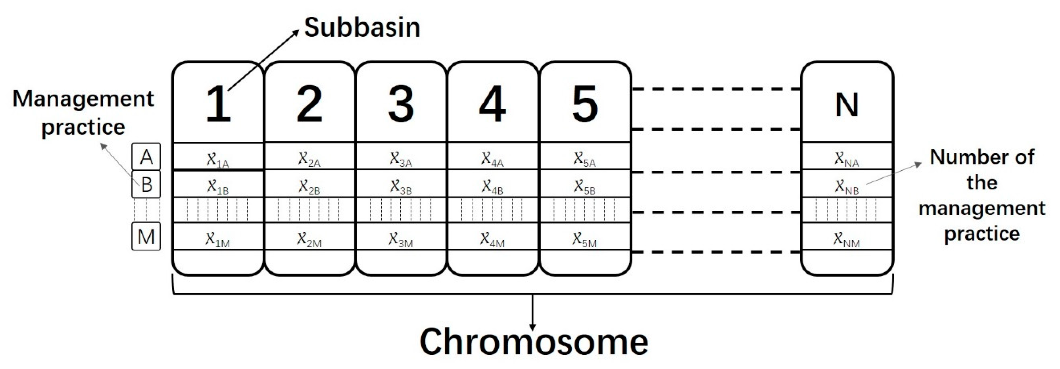
NSGAII generates offspring using a specific type of crossover and mutation and selects the next generation according to non-dominated sorting and crowding distance comparison. Figure 2 illustrates the genetic encoding of the various measure’s structures for arrangement of conservation practices in the optimization algorithm. The sub-basins delineated by RGWLF and the configurations of management practices in each sub-basin form the basic chromosome units. The length of each chromosome is equal to the total number of sub-basins.

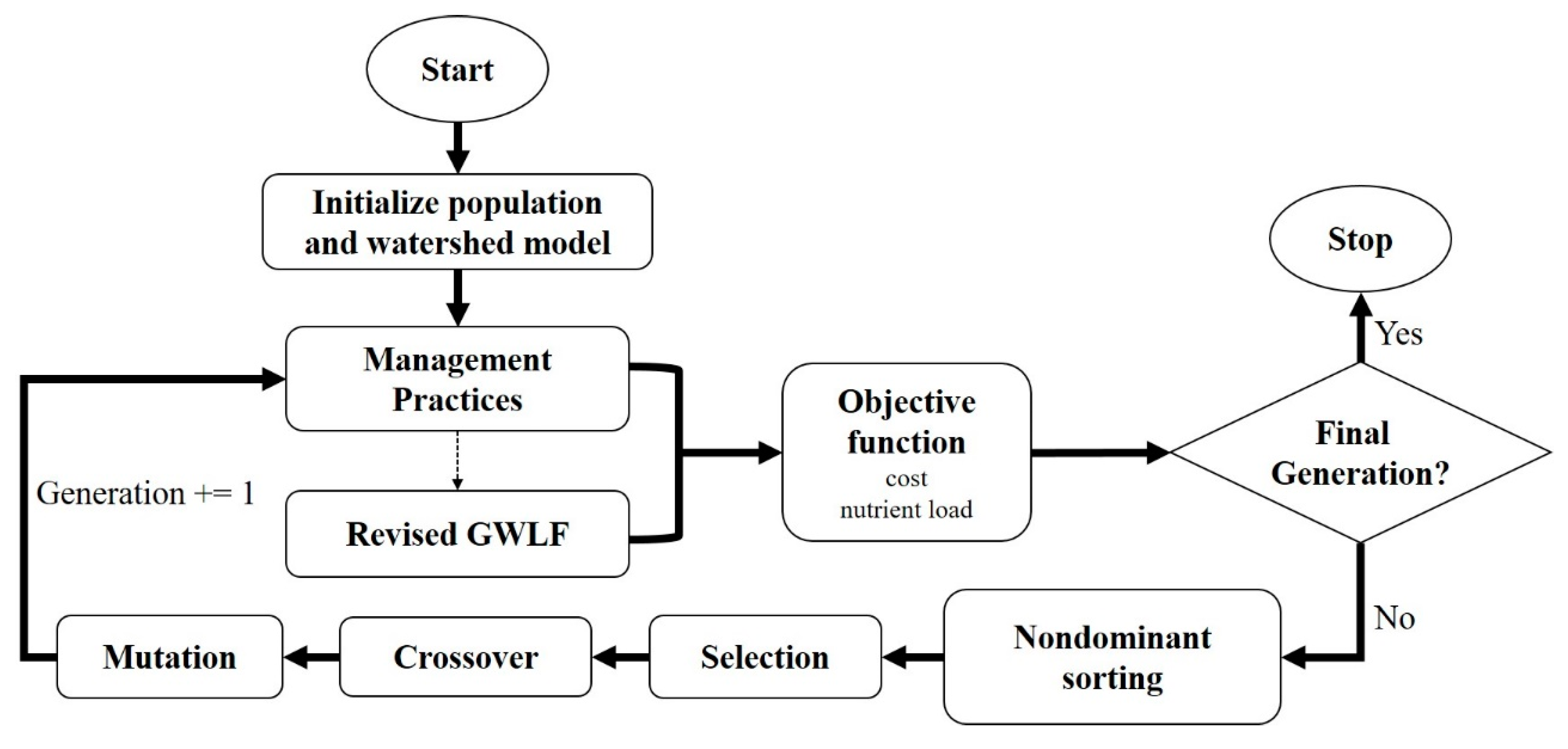
The analytical flow chart for this research is outlined in Figure 3. The watershed model was created to provide the nutrient load; the cost of management practices will be calculated by referring to the policy literature and actual surveys. To obtain the most cost-effective set of BMPs, the operation must satisfy two objective functions—the minimization of net total cost and the lowest dissolved nitrogen load—which are expressed by the equations:

$$\min ={{\displaystyle \sum }}_{\mathrm{i}=1}^{\mathrm{n}}{\mathrm{Cost}}_{\mathrm{pns},\mathrm{i}}+{\mathrm{Cost}}_{\mathrm{lu},\mathrm{i}}+{\mathrm{Cost}}_{\mathrm{strip},\mathrm{i}},$$

(7)

$$\min ={{\displaystyle \sum }}_{\mathrm{i}=1}^{\mathrm{n}}{\mathrm{DisN}}_{\mathrm{i},\mathrm{BMPs}},$$

(8)

where Cost_pns,i, Cost_lu,i, and Cost_strip,I are the costs of wastewater treatment plant, converting land-use, and bank filter strisp in sub-basin i; and DisN_i,BMPs is the total dissolved nitrogen load in sub-basin i.

The optimization process consists of several procedures, as follows:

(1)

Initialize the population and read the watershed model input data. Then, simulate the baseline scenario.

(2)

For the two objective functions, obtain the pollutant load of the basin model and the net cost of each management measure combination.

(3)

Through a series of processes, including non-dominated sorting, calculation of crowded distance, selection, crossover, and mutation, NSGAII obtains the Pareto-optimal result set of the current generation.

(4)

Repeat the second process, determine whether it is the last generation, and then perform the third process.

3. Results and Discussion

3.1. RGWLF Model Calibration and Validation

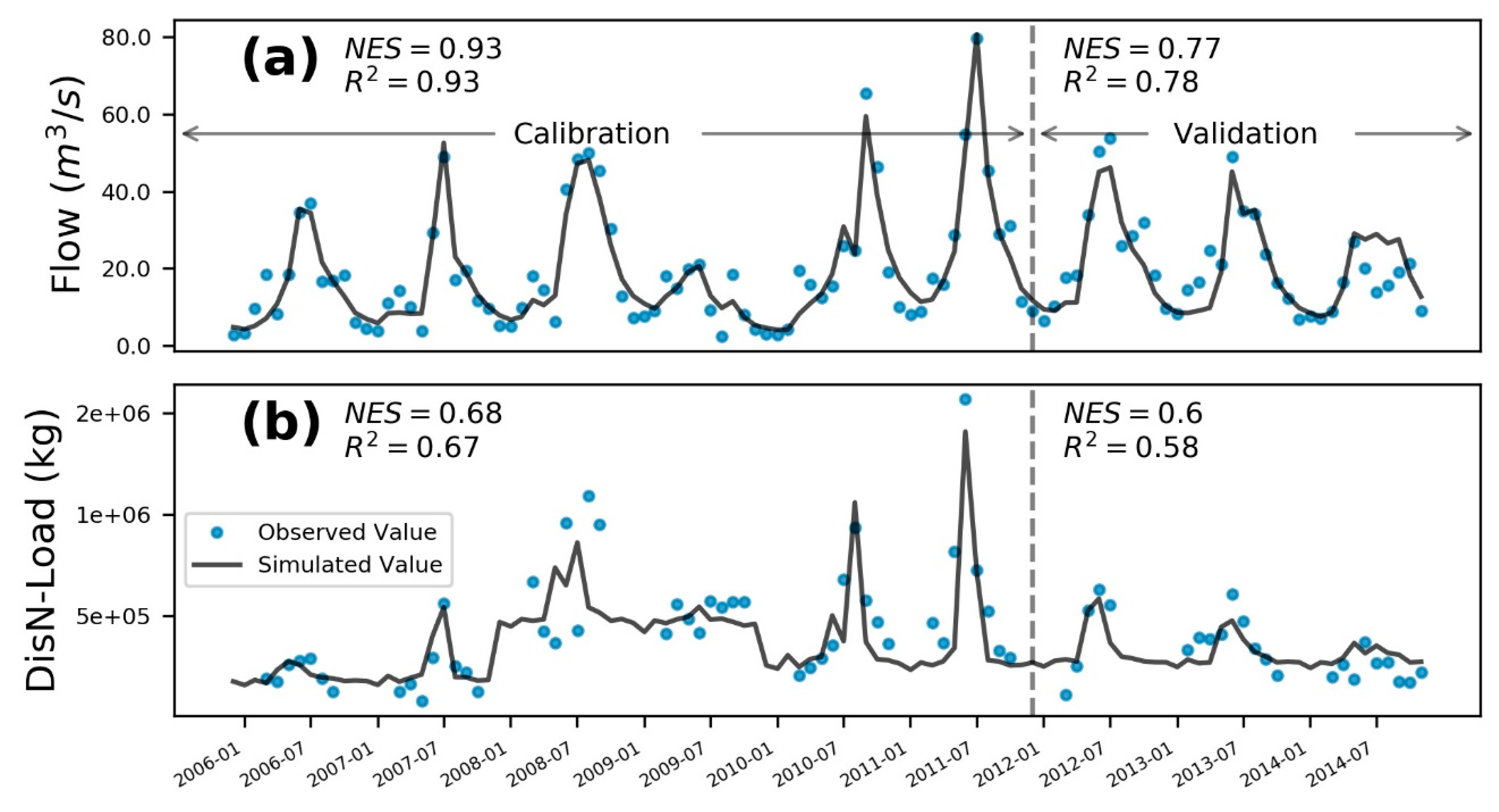
Nine years of monthly records of observed streamflow and dissolved nitrogen data were used for model calibration and verification at the outlet of the watershed. The simulation period was from 2005–2014, in which the first year (2005) was used as a warming-up period, the data from 2006–2011 were used for the calibration process, and the rest were used for model validation.

The generalized likelihood uncertainty estimation (GLUE), a frequently used Bayesian parameter estimation method, was used for calibration analysis in terms of both hydrology and pollutants for the watershed model [30,31].

Table 3. Parameters selected for the calibration.

Parameters Name	Initial	Range	Calibration
Recession coefficient	0.008	[0, 0.015]	0.00782
Seepage coefficient	0.01	[0, 0.02]	0.00671
Recession threshold	10	[0, 20]	17.784
Seepage threshold	10	[0, 20]	6.497
Leakage coefficient	0.06	[0, 0.08]	0.0436
CN2 1	-	[−0.15, 0.15]	−0.0418
Agriculture	75	-	-
Forest	35	-	-
Grass	45	-	-
Urban	95	-	-
Dissolved nitrogen Concentration (mg/L)	-	-	-
Agriculture	4.0	[2.0, 6.0]	4.66
Forest	0.2	[0.1, 0.3]	0.12
Grass	2.0	[1.0, 3.0]	1.76
During fertilizer (mg/L) Agriculture	10.0	[7.0, 15.0]	12.47
Underground dissolved nitrogen concentration	0.1	[0.01, 0.5]	0.24
Dissolved nitrogen attenuation exponent	0.0004	[0.0, 0.0008]	0.000233

¹ Relative changes apply to the CN2 range.

lists the uniform prior distribution range and best value for each calibrated parameter after 10,000 iterations. The Nash–Sutcliffe efficiency (NES) and the coefficient of determination (R²) were selected as the simulation evaluation criteria [32]. NSE can range from minus infinity to 1 and an efficiency of 1 indicates a perfect performance. R² ranges from 0 to 1, with higher values indicating a better fit for the model.

As shown in Figure 4, during the calibration period, the NES was 0.93 for streamflow and 0.68 for DisN; moreover, the R² values were 0.93 and 0.68 for the simulated streamflow and DisN, respectively. At the same time, the model validation for the streamflow R² and NES were 0.77 and 0.78, respectively. Similar to streamflow, DisN had a lower validation value of 0.60 for R² and 0.58 for NES. Both streamflow and DisN simulations by the model had a good performance on a monthly time scale, which indicates robustness of the RGWLF model, according to previous research [33].

3.2. Sensitivity Analysis of NSGAII Operational Parameters

To ensure accuracy of the NSGAII and optimization operational efficiency, sensitivity analyses were performed for the four key parameters, including population size, generations, crossover, and mutation probability, by the one-at-a-time sensitivity analysis method [16,34].

Table 4. Parameters selected for sensitivity analysis of non-dominated sorting genetic algorithms II (NSGAII).

Order	Population Size	Generations	Crossover Probability	Mutation Probability
1	30	50	0.1	0.001
2	40	80	0.3	0.005
3	50	100	0.5	0.01
4	80	200	0.7	0.03
5	100	500	-	0.05
6	200	-	-	0.08
default	80	100	0.5	0.01
optimal	50	200	0.5	0.03

lists the default and per-change values for the four NSGAII parameters.

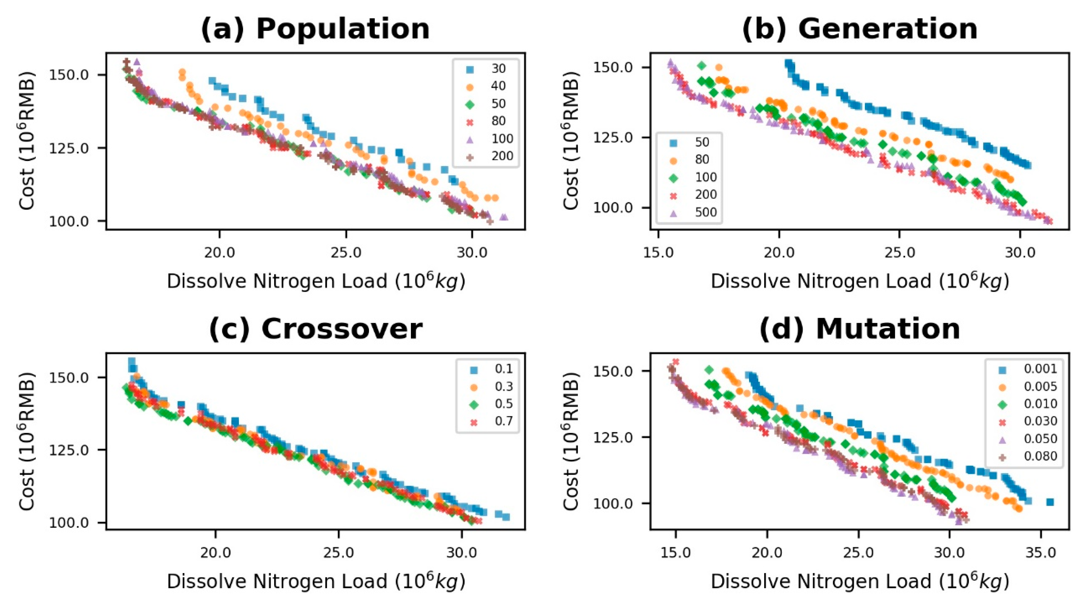
Figure 5a–d illustrate the Pareto-optimal fronts under per-change for the four key parameters. It is apparent in Figure 5a that the improvement in the Pareto-optimal fronts was remarkable as the population size increased from 30 to 50, but there was little gap for Pareto-optimal fronts when the population size was increased from 80 to 200. The main reason for this case is possibly that a population size of 50 had enough convergence chance for the solution space’s freedom of the whole optimization system. Furthermore, a value of 50 would considerably reduce the computation time, compared to the default values of 80, 100 and 200.

As shown in Figure 5b, the number of generations also had an appreciable impact on the Pareto-optimal fronts. A significant improvement in the Pareto-optimal front was noticed, with the number of generations increasing from 50 to 200. In stark contrast, increasing from 200 to 500 did not bring any improvement for the Pareto-optimal fronts.

Unlike the above two parameters, the Pareto-optimal front was not sensitive to changes in the crossover probability, which is displayed in Figure 5c. The Pareto-optimal front had an inconspicuous shift approaching the origin as the crossover probability increasing from 0.1 to 0.5. When the crossover probability reached a value of 0.7, the Pareto-optimal front was farther away from the origin.

The trend of the Pareto-optimal front, as affected by the change of Mutation probability, is presented in Figure 5d. What stands out most in this figure is that mutation probability is a sensitive parameter, especially in the range from 0.001 to 0.03, where the Pareto-optimal front approached the origin with an increase of parameter value. However, there was no benefit for the Pareto-optimal front as the parameter increased from 0.03 to 0.08.

Considering all of the above analyses, the values 50, 200, 0.5 and 0.03 were used as population size, generations, crossover, and mutation probability, respectively, for the further optimization processes.

3.3. Optimization Result and Cost-Effectiveness Analysis

The baseline scenario for this watershed was no management practice and 4.05 × 10⁷ kg for the total dissolved nitrogen load over nine years.

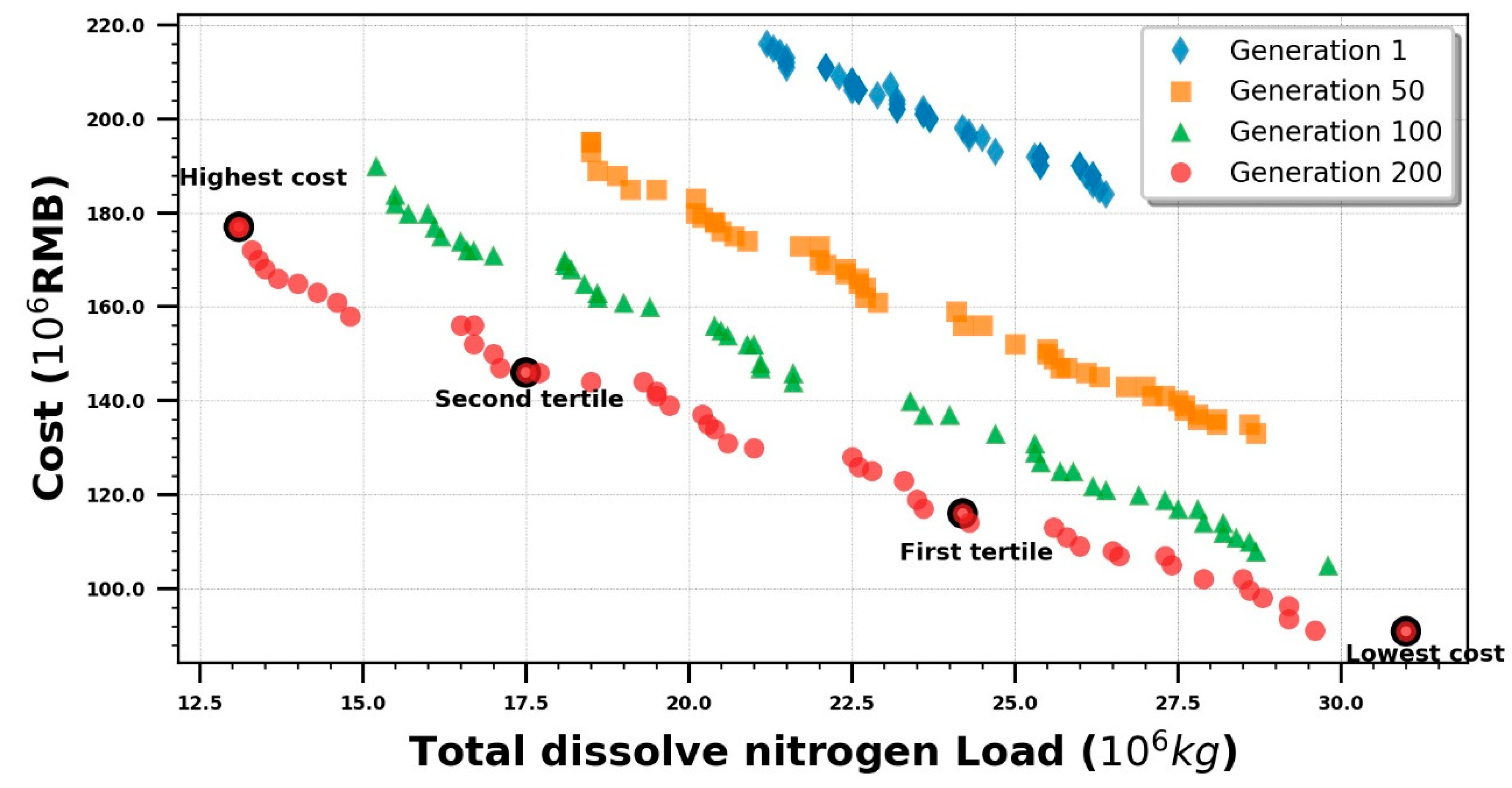
Figure 6 provides the final optimization progress with two objectives, minimizing the net cost and dissolved nitrogen load by scattering four Pareto-optimal fronts belonging to four generations (1, 50, 100 and 200). The overall trend for the four scatter diagrams was that the dissolved nitrogen decreased as the net cost increased. Each new generation’s chromosomes were initialized by random numbers without no optimization process (such as non-dominance, selection, crossover, and so on), so it was regarded as the 0th generation and not shown in the figure. In the first generation, the distribution of points was more concentrated, indicating that the solutions were less differentiated. As the number of generations increased, the solution became more and more scalable, and came closer to the origin. For the final generation, the most widespread solution set, which was closest to the origin, can be seen. Thus, the best quality and broadest decision supports were supplied to the policy researchers and decision-makers.

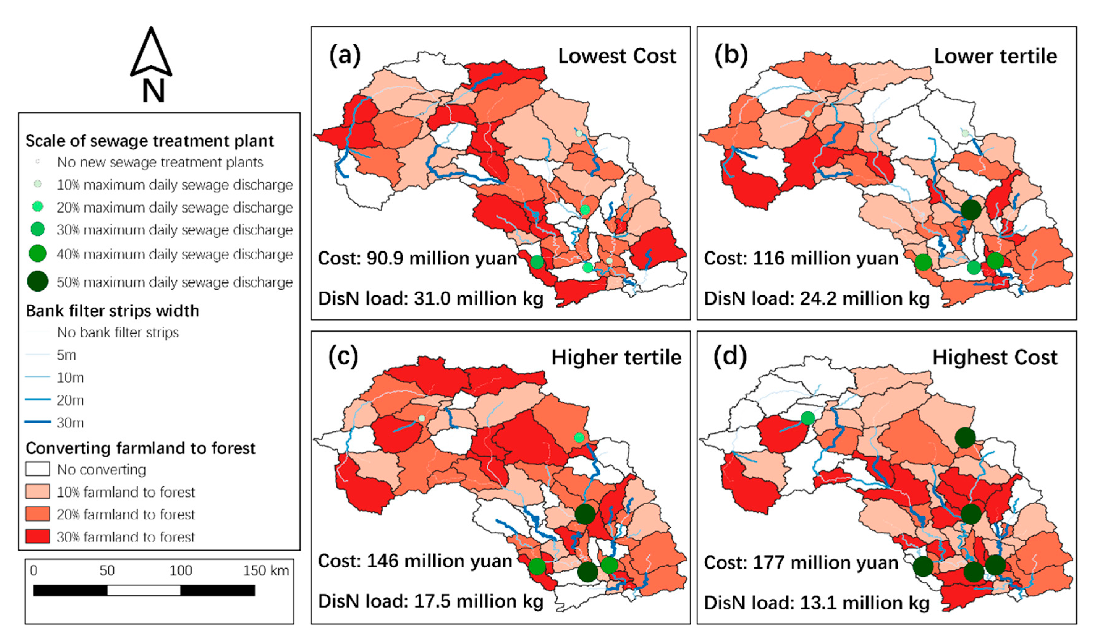
The set of solutions was divided into three segments with four endpoints, which were: the lowest cost, the lower tertile cost point, the higher tertile cost point, and the highest cost. The values of cost, dissolved nitrogen load, and spatial distribution of corresponding management measures for the four scenarios are shown in Figure 7. For the lowest cost scenario (Figure 7a), the scale of treatment of polluted water plants is small and the measures are mainly bank filter strips and converting farmland to forest. As cost increased, the intensity and scale of management practices also increased, which is illustrated in Figure 7b,c. At the point of maximum cost (Figure 7d), the load of dissolved nitrogen reached its minimum value, where the designed daily treatment capacity of the sewage plant was extremely high and there was no conversion of farmland to forests in some upstream sub-basins. The majority of management practices are concentrated in middle and lower regions of the watershed.

4. Conclusions

In this study, we supplemented the RGWLF model with the addition of a pollutant attenuation process in the river channel and a bank filter strips reduction function, based on our previous research. Meanwhile, taking into account the regional pollution source composition of the watershed studied and the characteristics of the models used, three types of pollution control measures—point source wastewater treatment, bank filter strips, and converting farmland to forest—were considered, and the cost of each measure was determined. Furthermore, the optimization algorithm NGSAII was linked with the RGWFL watershed model and the implemented measures to search for a Pareto-optimal set of BMPs. Before the final optimization calculation, sensitivity analyses for the four key parameters of NGSAII were performed. According to the results of the sensitivity analysis, the entire coupled model system supplied 50 solutions which could provide managers with many pollution reduction options. In the end, depending on the cost, we chose four gradient solutions and demonstrated the geospatial distribution of their different management measure characteristics and briefly analyzed the differences and features of the four solutions.

The research results show that, with almost no increase in data requirements, dissolved nitrogen had an excellent simulation performance, expanding the spatial scope of pollutant simulation for the GWLF. Moreover, due to its robustness and semi-distribution, the RGWLF model was able to be coupled with NSGAII. The entire linkage system had good performance in the optimization process and provided a range of watershed implementation measures for DisN reduction and minimizing cost, which is a worthy reference for policy researchers and decision-makers to realize their watershed management goals. However, limited by the available data, funding, and researchers’ capabilities, we did not consider other target indicators, such as sediment, phosphorus, and so on, which could be carried out in future research.

References

- Gleick, P.H. Global freshwater resources: Soft-path solutions for the 21st century. Science 2003, 302, 1524–1528. [Google Scholar] [CrossRef] [Green Version]
- Fleifle, A.; Saavedra, O.; Yoshimura, C.; Elzeir, M.; Tawfik, A. Optimization of integrated water quality management for agricultural efficiency and environmental conservation. Environ. Sci. Pollut. Res. 2014, 21, 8095–8111. [Google Scholar] [CrossRef]
- Borah, D.K.; Bera, M. Watershed-scale hydrologic and nonpoint-source pollution models: Review of applications. Trans. ASAE 2004, 47, 789–803. [Google Scholar] [CrossRef] [Green Version]
- Hering, D.; Borja, A.; Carstensen, J.; Carvalho, L.; Elliott, M.; Feld, C.K.; Heiskanen, A.-S.; Johnson, R.K.; Moe, J.; Pont, D.; et al. The European Water Framework Directive at the age of 10: A critical review of the achievements with recommendations for the future. Sci. Total Environ. 2010, 408, 4007–4019. [Google Scholar] [CrossRef] [Green Version]
- Qu, J.; Fan, M. The current state of water quality and technology development for water pollution control in China. Crit. Rev. Environ. Sci. Technol. 2010, 40, 519–560. [Google Scholar] [CrossRef]
- Xie, H.; Chen, L.; Shen, Z. Assessment of agricultural best management practices using models: Current issues and future perspectives. Water 2015, 7, 1088–1108. [Google Scholar] [CrossRef] [Green Version]
- Balana, B.B.; Vinten, A.; Slee, B. A review on cost-effectiveness analysis of agri-environmental measures related to the EU WFD: Key issues, methods, and applications. Ecol. Econ. 2011, 70, 1021–1031. [Google Scholar] [CrossRef]
- Guo, H.; Hu, Q.; Jiang, T. Annual and seasonal streamflow responses to climate and land-cover changes in the Poyang Lake basin, China. J. Hydrol. 2008, 355, 106–122. [Google Scholar] [CrossRef]
- Hundecha, Y.; Bardossy, A. Modeling of the effect of land use changes on the runoff generation of a river basin through parameter regionalization of a watershed model. J. Hydrol. 2004, 292, 281–295. [Google Scholar] [CrossRef]
- Deb, K. Multi-objective genetic algorithms: Problem difficulties and construction of test problems. Evol. Comput. 1999, 7, 205–230. [Google Scholar] [CrossRef] [PubMed]
- Kaini, P.; Artita, K.; Nicklow, J.W. Optimizing structural best management practices using SWAT and genetic algorithm to improve water quality goals. Water Resour. Manag. 2012, 26, 1827–1845. [Google Scholar] [CrossRef]
- Qi, H.; Altinakar, M.S.; Vieira, D.A.N.; Alidaee, B. Application of Tabu search algorithm with a coupled AnnAGNPS-CCHE1D model to optimize agricultural land use. J. Am. Water Resour. Assoc. 2008, 44, 866–878. [Google Scholar] [CrossRef]
- Muleta, M.K.; Nicklow, J.W. Decision support for watershed management using evolutionary algorithms. J. Water Resour. Plan. Manag. 2005, 131, 35–44. [Google Scholar] [CrossRef]
- Qiu, J.; Shen, Z.; Huang, M.; Zhang, X. Exploring effective best management practices in the Miyun reservoir watershed, China. Ecol. Eng. 2018, 123, 30–42. [Google Scholar] [CrossRef]
- Deb, K.; Pratap, A.; Agarwal, S.; Meyarivan, T. A fast and elitist multiobjective genetic algorithm: NSGA-II. IEEE Trans. Evol. Comput. 2002, 6, 182–197. [Google Scholar] [CrossRef] [Green Version]
- Maringanti, C.; Chaubey, I.; Arabi, M.; Engel, B. Application of a multi-objective optimization method to provide least cost alternatives for NPS pollution control. Environ. Manag. 2011, 48, 448–461. [Google Scholar] [CrossRef]
- Maringanti, C.; Chaubey, I.; Popp, J. Development of a multiobjective optimization tool for the selection and placement of best management practices for nonpoint source pollution control. Water Resour. Res. 2009, 45. [Google Scholar] [CrossRef] [Green Version]
- Ahmadi, M.; Arabi, M.; Hoag, D.L.; Engel, B.A. A mixed discrete-continuous variable multiobjective genetic algorithm for targeted implementation of nonpoint source pollution control practices. Water Resour. Res. 2013, 49, 8344–8356. [Google Scholar] [CrossRef]
- Geng, R.; Yin, P.; Sharpley, A.N. A coupled model system to optimize the best management practices for nonpoint source pollution control. J. Clean. Prod. 2019, 220, 581–592. [Google Scholar] [CrossRef]
- Wellen, C.; Kamran-Disfani, A.-R.; Arhonditsis, G.B. Evaluation of the current state of distributed watershed nutrient water quality modeling. Environ. Sci. Technol. 2015, 49, 3278–3290. [Google Scholar] [CrossRef]
- Arabi, M.; Govindaraju, R.S.; Hantush, M.M. Cost-effective allocation of watershed management practices using a genetic algorithm. Water Resour. Res. 2006, 42. [Google Scholar] [CrossRef] [Green Version]
- Qi, H.; Altinakar, M.S. Vegetation buffer strips design using an optimization approach for non-point source pollutant control of an agricultural watershed. Water Resour. Manag. 2011, 25, 565–578. [Google Scholar] [CrossRef]
- Qi, Z.; Kang, G.; Chu, C.; Qiu, Y.; Xu, Z.; Wang, Y. Comparison of SWAT and GWLF model simulation performance in humid south and semi-arid north of China. Water 2017, 9, 567. [Google Scholar] [CrossRef] [Green Version]
- Qi, Z.; Kang, G.; Shen, M.; Wang, Y.; Chu, C. The improvement in GWLF model simulation performance in watershed hydrology by changing the transport framework. Water Resour. Manag. 2019, 33, 923–937. [Google Scholar] [CrossRef]
- Haith, D.A.; Shoemaker, L.L. Generalized watershed loading functions for stream flow nutrients. JAWRA J. Am. Water Resour. Assoc. 1987, 23, 471–478. [Google Scholar] [CrossRef]
- Schwarz, G.; Hoos, A.B.; Alexander, R.; Smith, R. The SPARROW surface water-quality model—Theory, application and user documentation. In U.S. Geological Survey Techniques and Methods; Series number 6-B3; U.S. Geological Survey: Reston, VA, USA, 2006; 248p. [Google Scholar]
- Shi, H.; Wang, L. Treatment of the corn starch wastewater by UASB-SBR process. Shanxi Archit. 2003, 29, 71–72. (In Chinese) [Google Scholar]
- Yu, H. UASB-SBR Technical Processing Starch Wastewater. Master’s Thesis, Changan University, Xi’an, China, 2007. (In Chinese). [Google Scholar]
- Liu, J.; Zheng, X.; Gao, C.; Chen, L. Study on area, operating and construction costs of urban wastewater treatment plants. Chin. J. Environ. Eng. 2010, 4, 2522–2526. (In Chinese) [Google Scholar]
- Beven, K.; Binley, A. The future of distributed models: Model calibration and uncertainty prediction. Hydrol. Process. 1992, 6, 279–298. [Google Scholar] [CrossRef]
- Beven, K.; Smith, P.; Freer, J. Comment on “Hydrological forecasting uncertainty assessment: Incoherence of the GLUE methodology” by Pietro Mantovan and Ezio Todini. J. Hydrol. 2007, 338, 315–318. [Google Scholar] [CrossRef]
- Nash, J.E.; Sutcliffe, J.V. River flow forecasting through conceptual models part I—A discussion of principles. J. Hydrol. 1970, 10, 282–290. [Google Scholar] [CrossRef]
- Moriasi, D.N.; Arnold, J.G.; Van Liew, M.W.; Bingner, R.L.; Harmel, R.D.; Veith, T.L. Model evaluation guidelines for systematic quantification of accuracy in watershed simulations. Trans. ASABE 2007, 50, 885–900. [Google Scholar] [CrossRef]
- Hamby, D. A comparison of sensitivity analysis techniques. Health Phys. 1995, 68, 195–204. [Google Scholar] [CrossRef] [PubMed] [Green Version]
Figure 1.
Location, sub-basins, land-use distribution, and elevation of the Luanhe watershed.
Figure 2.
Gene string (chromosomes) for best management practices (BMPs) optimization in the watershed.
Figure 3.
The optimization process for BMP selection and placement.
Figure 4.
Time-series for the entire period (2006–2014) of observed and simulated monthly streamflow (a) and dissolved nitrogen (b).
Figure 5.
Pareto-optimal fronts for the sensitivity analysis of NSGAII.
Figure 6.
Pareto-optimal fronts for total dissolved nitrogen load and cost.
Figure 7.
The types and locations of optimal BMPs for different costs, as provided in Figure 6.