Article

Hydrogeomorphic Impacts of Floods in a First-Order Catchment: Integrated Approach Based on Dendrogeomorphic Palaeostage Indicators, 2D Hydraulic Modelling and Sedimentological Parameters

Department of Physical Geography and Geoecology, Faculty of Science, University of Ostrava, Chittussiho 10, 710 00 Ostrava, Czech Republic
*
Author to whom correspondence should be addressed.
Water 2020, 12(1), 212; https://doi.org/10.3390/w12010212
Submission received: 22 November 2019 / Revised: 6 January 2020 / Accepted: 10 January 2020 / Published: 12 January 2020

Abstract

:
Floods represent frequent hazards in both low- and first-order catchments; however, to date, the investigation of peak flow discharges in the latter catchments has been omitted due to the absence of gauging stations. The quantification of flood parameters in a first-order catchment (1.8 km2) was realised in the moderate relief of NE Czechia, where the last flash flood event in 2014 caused considerable damage to the infrastructure. We used an integrated approach that included the dendrogeomorphic reconstruction of past flood activity, hydraulic modelling of the 2014 flash flood parameters using a two-dimensional IBER model, and evaluation of the channel stability using sedimentological parameters. Based on 115 flood scars, we identified 13 flood events during the period of 1955 to 2018, with the strongest signals recorded in 2014, 2009 and 1977. The modelled peak flow discharge of the last 2014 flood was equal to 4.5 m3·s−1 (RMSE = 0.32 m) using 26 scars as palaeostage indicators. The excess critical unit stream power was observed at only 24.2% of the reaches, representing predominantly bedrock and fine sediments. Despite local damage during the last flood, our results suggest relatively stable geomorphic conditions and gradual development of stream channels under discharges similar to that in 2014.

1. Introduction

Extreme rainfall resulting in flood events is a common phenomenon in different environments, including both mountain ranges and lowlands [1,2]. The systematic monitoring of flow stages at gauging stations, including precipitation and flow discharge prediction, is currently well applied and documented in many medium- and large-sized rivers [3,4,5]. In contrast, data from mountain steep headwater catchments and, in general, first-order catchments [6] are still poor, due to the insufficient network of stream gauges and the sporadic amount of processed documentary evidence [7]. Not only do mountain headwater streams generate sediment-laden flows with aftermaths within and along fans [8,9], but also streams and gullies of first-order catchments (up to 10 km2) in moderate relief can be responsible for local damage to infrastructure. Ozturk et al. [10] analysed extraordinary flash flood events (140 mm per 2 h) in a small catchment (6 km2) that resulted in damage to infrastructure and a high amount of suspended sediments (t/km2) due to intense hillslope–channel coupling. In addition, Terti et al. [11] pointed to a short response time of small catchments to flash floods, thereby increasing the probability of trapping people during outdoor activities.
Despite the lack of gauging records from forested first-order catchments, several approaches exist to describe the hydrogeomorphic impacts of extremely high flow stages. The dating of flood scars on riparian vegetation using dendrogeomorphic methods [12,13] and recording their position and height above the channel bottom with a combination of hydraulic models is a well-established approach for the estimation of peak flood discharge, flow velocity, and unit stream power [14]. Using flood scars as a palaeostage indicator (PSI; maximum height of the scar above the channel bottom) allowed the interpretation of past flood events in medium- and large-scale rivers (catchment areas larger than 40 km2), for example, in the Western Mediterranean [15], North America [16,17], the Carpathians [18], and the Himalayas [19]. The dendrogeomorphic response of flash floods in small catchments is generally considered lower [20] but may increase due to the presence of erodible sediments amplifying lateral bank erosion. In such conditions, while small streams may not generate flood waves as large as those of large rivers, the presence of exposed and scarred tree roots [21] may complete a relatively low number of scarred tree stems.
The alluvial streams draining first-order catchments often do not display clear relationships between channel geometry, bed substrate, unit stream power and drainage area, and their resulting form and evolution trajectory are unpredictable unless local conditions (e.g., bedrock resistance, intensity of hillslope-channel coupling processes, land use history, and presence of large instream wood) are constrained [22,23,24,25,26]. These streams are characterized by a more or less developed stepped-bed morphology with a wide range of sediment size, where individual steps controlling channel bed stability consist of interlocked boulders, bedrock outcrops or large wood pieces [27]. This implies the relative stability of their channel beds under relatively high discharges (up to floods of 20–50-year recurrence intervals) and thus only limited adjustments of the channel morphology and geometry to lower (e.g., bankfull) flows owing to the presence of generally shallow flows, particle-size interactions (hide/protrusion effect) and additional bed form resistance [25,28,29,30,31]. The correlations between the unit stream power, sediment calibre and prevailing fluvial process may exist at the reach scale when spatially limited depositional reaches can be accompanied by local bed sediment fining and an abrupt decrease in the unit stream power of a high-magnitude flood [23]. Nevertheless, our knowledge of the direct relationships between the transport capacity of a particular flood event, bed stability and the resulting fluvial processes in first-order catchments is still somewhat limited by the lack of detailed post-flood field surveys of geomorphic consequences.
As mentioned, two-dimensional hydraulic models have been successfully applied to peak discharge reconstructions in ungauged or poorly gauged catchments of various sizes and environments [18,32,33,34,35]. This peak discharge is mostly defined not as the single deterministic value but rather as a range of values due to uncertainties inherent in the process of the estimation [36]. Discharges predicted in such a way could be used in flood frequency analyses [18], where they serve as outliers to the measured discharges. Consequently, the predicted discharges could serve as a basis for the evaluation and mitigation of flood risk [34] or as information about the flood magnitude in the historical period [32]. Moreover, the results of hydraulic simulations can be used for the estimation of stream transport capacity and channel stability during a particular flood event at a very detailed scale. In this sense, the bed shear stress and unit stream power are relevant parameters for calculating the incipient motion of coarse bed particles and thus evaluating the stability of stepped-bed channels consisting of relatively stable cobble to boulder steps [30,37].
For our purposes, we selected a first-order catchment (1.8 km2) in the moderate relief of the Eastern Sudetes (NE Czechia), where, during the last 15 years, the occurrence of several flash flood events caused substantial geomorphic imprints [38]. In particular, the last intense precipitation event (27 May 2014) resulted in a moderate flood risk in the case of medium-sized rivers (2-year recurrence interval), but a discharge of an approximately 100-year recurrence interval was estimated at ungauged small streams. The short-lived storm, with a total rainfall amount of 40 mm (locally up to 80 mm), had an intensity of between 40 and 60 mm/h. Its hydrogeomorphic response was primarily due to unprecedented rainfall intensity and large antecedent precipitation. The financial costs of the flash flood aftermaths in the affected region were calculated as approximately EUR 200,000 [39].
Our aims were to (i) create the chronology of the flash flood events in this small catchment using dendrogeomorphic approaches, (ii) estimate the parameters (peak flow discharge, flow velocity, bed shear stress, and unit stream power) of the last 2014 flash flood event using the combination of PSI and 2D hydraulic modelling, and (iii) describe the stream transport capacity and channel stability during the 2014 flash flood event based on the hydraulic simulation data and sedimentological parameters. Such a comprehensive approach may help to better quantify the flash flood parameters of ungauged streams and thus contribute to more reliable management of small streams in future extreme climate events.

2. Materials and Methods
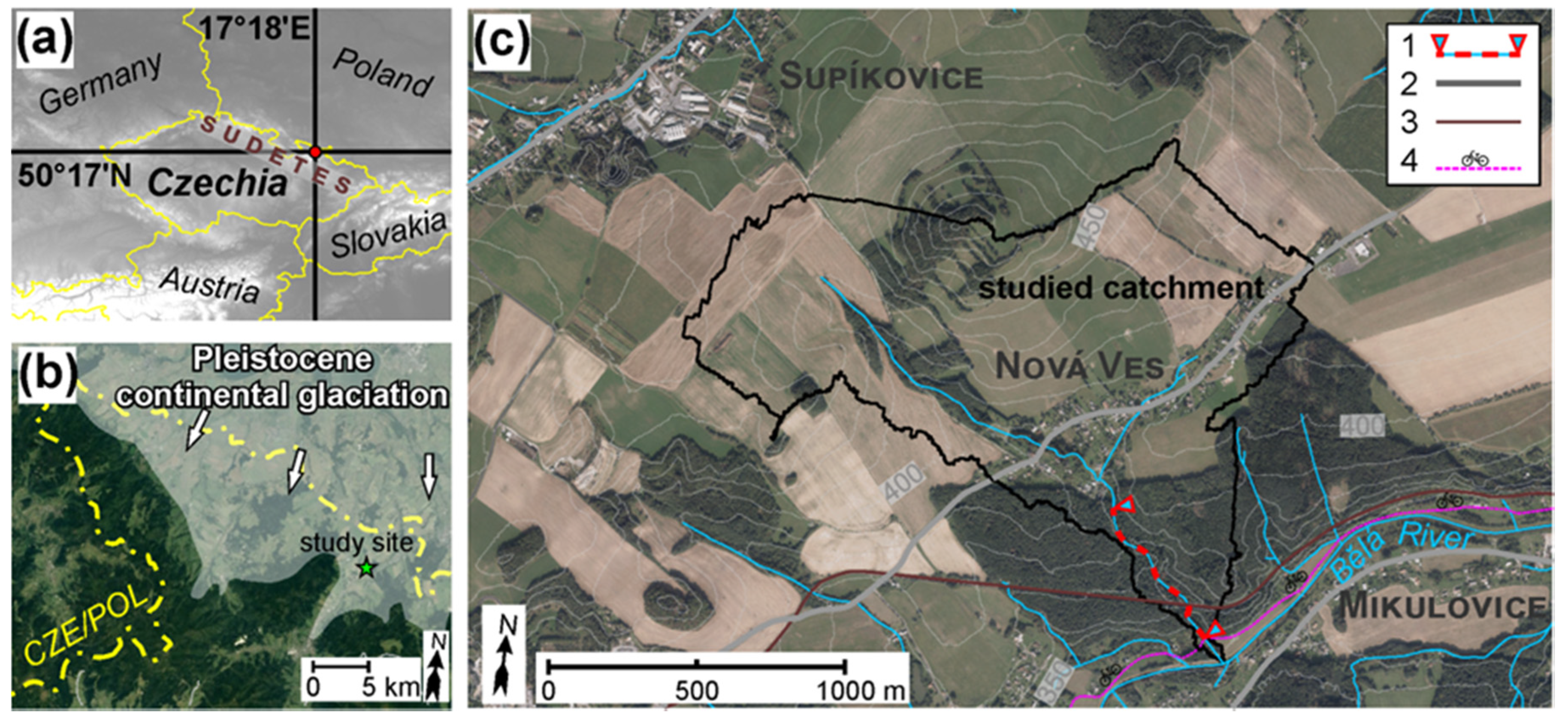
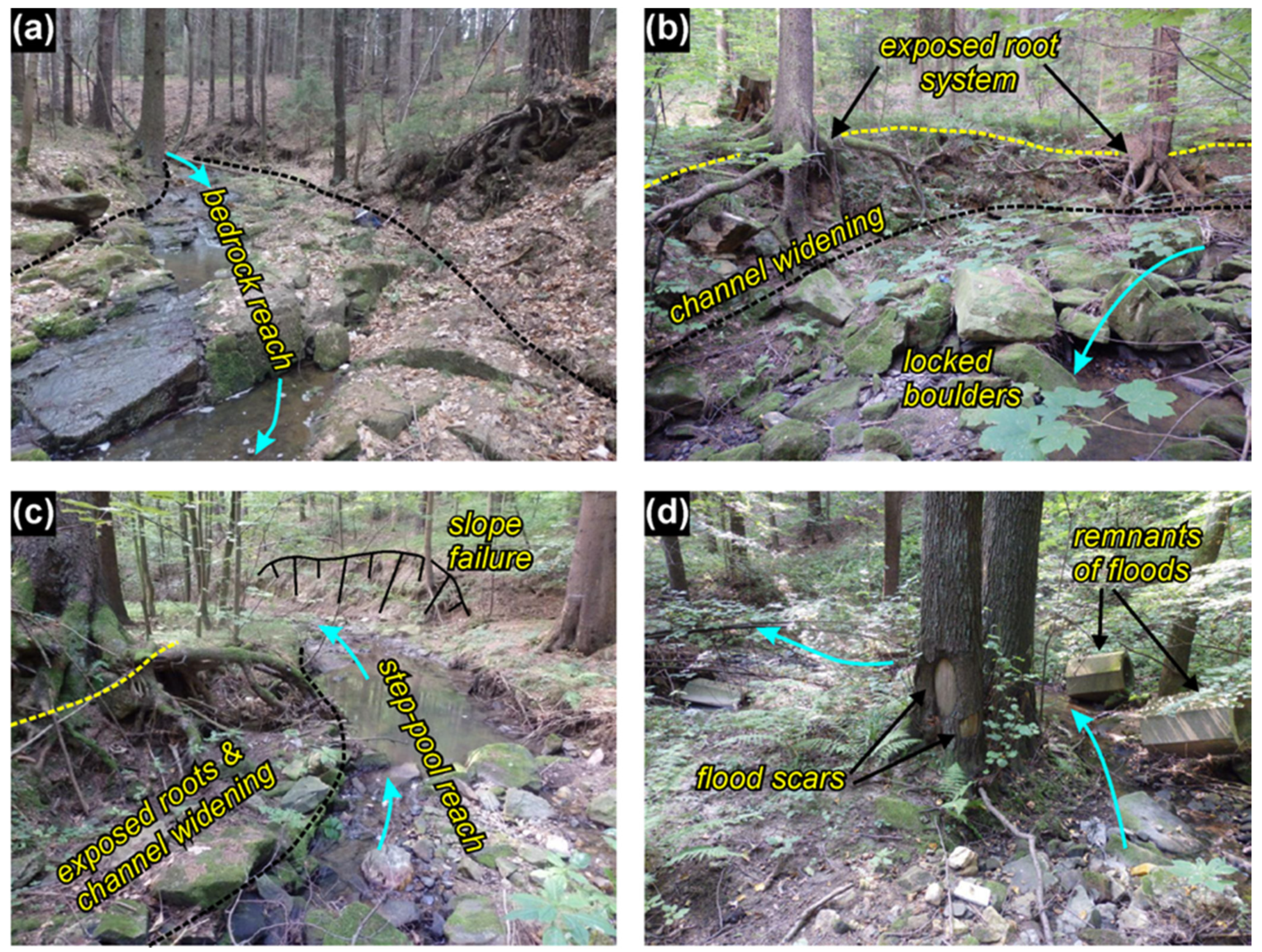
2.1. Study Site

The hydrogeomorphic impacts of floods were studied on a small tributary of the Bělá River in the foreland of the Eastern Sudetes (NE part of Czechia, Central Europe; 50°17′ N, 17°17′ E; Figure 1). The area comprises a Proterozoic and Palaeozoic basement composed of orthogneiss, which is overlaid by glacifluvial deposits of the Saalian and Elsterian glaciations with different grain-size distributions of till sediments. These deposits are the result of deglaciation phases in proglacial areas on the ice margins and were recently covered by the Holocene sandy loam colluvium [40,41]. The study site is characterised by a temperate climate, with a mean annual precipitation between 850 and 900 mm. Most precipitation falls during the spring and summer months [42], with an occasional occurrence of extreme daily rainfall (more than 50 mm per day). Documentary evidence provides information about several flood events (e.g., 1903, 1921, 1971, 1977, 2007, 2009, and 2014), relating to both advective rains and short-term intense rainfall events that are currently responsible for intense gully incision and damage to infrastructure within the studied region [38,43].
We focused on an approximate 700-m-long reach of an unnamed first-order stream draining a catchment area of 1.8 km2 with a mean elevation of 417.5 m a.s.l. Fields and dwellings dominate the upper and middle catchment area, while the lower part (i.e., the study reach) is predominantly covered by a mixed forest (Figure 1c). The mean stream gradient of the study reach is 0.05 m/m, with a maximum up to 0.17 m/m. The channel cuts into the Pleistocene and Holocene deposits, with typical alternations of stepped-bed morphology and bedrock outcrops (Figure 2a) accompanied by poorly sorted bed sediments (Figure 2b,c). Fresh slope/bank failures (up to 50 m long and 10 m high) and generally unstable banks have caused channel widening during recent floods, resulting in the frequent occurrence of exposed tree root systems and flood scars on riparian vegetation along the entire reach (Figure 2b–d). In contrast, there is no evidence of deep channel incision due to the resistant gneiss bedrock and large interlocked boulders at several reaches within the stream. Slopes and floodplains surrounding the channel are overgrown by a mixed forest composed predominantly of Pinus sylvestris L., Picea abies (L.) Karst., Alnus glutinosa (L.) Gaertn, and Tilia cordata Mill. At 0.5 river km (r. km), the stream drains to a 50-m-long concrete trough within a viaduct under a railway. Moreover, culverts are presented under a cycle path in the lower part and under a road through a village in the middle part of the catchment.

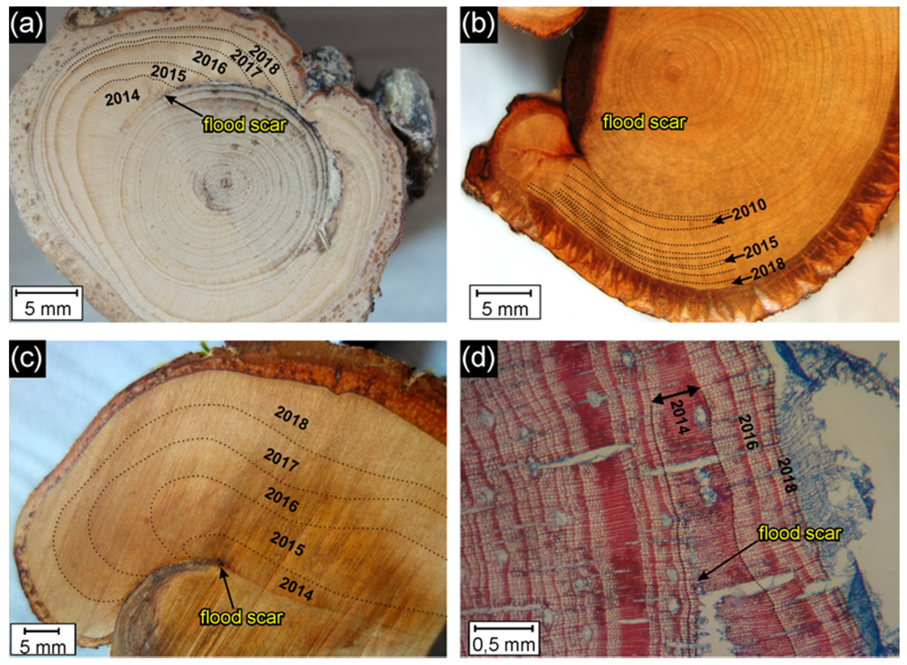
2.2. Dendrogeomorphic Fieldwork and Analyses

First, the terrain fieldwork focused on dendrogeomorphic sampling to create the chronology of past flood events and to select the flood scars caused by the 2014 flood event. The tree sampling followed the standard dendrogeomorphic procedure for flood reconstruction [13,44]. The sampling was focused on flood scars occurring either on tree stems or exposed tree roots. In the case of tree stems, increment cores were extracted from the edge of the scar and from the undisturbed part of the tree stem using the Pressler increment borer (40 × 0.5 mm). Tree stems of a small diameter (up to 10 cm) were cut by handsaw in the position of the flood scar to gain the stem disc or wedge while approximately 2-cm-wide cross-sections were sampled from exposed and scarred living roots. Only those scars oriented against the supposed direction of the flow path were considered for sampling. In addition, only scars that occurred on exposed but stabilized roots with the lowest tendency to flex during higher discharges were used to avoid the underestimation of modelled peak flow discharge [45]. All sampled trees were carefully described, and the height of the sampled scar was carefully noted, labelled with a visible object, photographed, and targeted using GPS. Reference trees growing near the study reach without any geomorphic influence on tree growth were sampled to cross-date with the disturbed samples and to eliminate false and missing rings.
Laboratory processing followed the standard dendrogeomorphic procedure [13,46]. All increment cores were glued into woody supports and—together with cross sections—dried and polished to be ready for dendrogeomorphic analysis. The tree rings of the increment cores and stem discs were counted and measured using TimeTable and PAST4 software [47], and their growth patterns were compared with the appropriate reference chronology (compiled in Arstan software [48] using a double detrending procedure) to ensure the reliability of dating. As root segments are more problematic regarding the occurrence of missing and wedging rings, the zig-zag segment tracing method [49] was applied to carefully count the years of each ring. In the case of problematic roots (i.e., dense growth increment and small roots), we used microslides cut by GLS-1 microtome and processed according to standard chemical procedures to precisely define the position of the flood scar within the root section [50,51].
In the next step, we identified the years with the occurrence of scars and onset of callus tissues (Figure 3) and compiled the chronology of past flood events. Scars represent an unequivocal signal of flood events and are considered the most reliable growth disturbance in dendrogeomorphic flood reconstructions [44]. The event identification was based on the event-response index (It index [52]), calculated as:
I t = R t A t × 100 %
where R is the number of scars in a year t and A is the total number of sampled trees living in a year t. Then, a certain event was considered when It ≥ 10% and the number of scars ≥ 3, while a probable event was determined when 10% > It ≥ 5% and the number of scars ≥ 2. From the whole dataset of scars, we eventually selected the scars dated to 2014 as a PSI of the May 2014 flash flood event, whose parameters were modelled.

2.3. Channel Parameters and Channel Geometry

This part consisted of (i) the measurement of the longitudinal profiles (channel/floodplain geometry) to model the 2014 flood behaviour and (ii) the classification of erosive/depositional segments and the measurement of the largest clasts for the determination of channel stability during the 2014 floods:
(i) The channel/floodplain geometry and the height of the 2014 scars (PSI) were measured in cross sections using a total station (GTS-212) with an accuracy of ±2.5 cm and a GNSS geodetic receiver (Trimble R2) with an accuracy of ±4 cm. All measurements were taken in the spring of 2019. To register the complexity of the channel geometry, the density of cross sections was as follows: the position of the first cross section was located directly in the position of the scars. Afterwards, five cross sections were measured, with the distance of one meter among each other, followed by two cross sections at a distance of 2.5 m and one cross section at a distance of 5 m. Next, cross sections were measured at a distance of 10 m. In the case of close distances between the scars, no overall process was applied. In total, 341 cross sections were measured, resulting in 4300 surveyed points. The GNSS geodetic receiver was only applied to place the relative position of points to the absolute location based on the local geographical reference system. A digital terrain model (DTM) in raster format was created from these cross sections with a grid size equal to 0.1 m and was used as a source for the hydraulic modelling.
(ii) To reveal the channel stability during the last flood event, the middle axes of the five largest bed particles were measured by a tape (with ±0.01 m accuracy; with a less-precise ±0.05 m accuracy only in a few cases of partially buried boulders) in 10 ± 1 m intervals along the stream’s longitudinal profile, except for the reach located in the culvert (0.51–0.54 r. km). Only the particles within the bankfull channel were accounted for. Consequently, the representative mean boulder diameter MBD (mm) for each of the channel cross sections was calculated as the arithmetical mean of these five measurements [23]. We classified each cross section as erosional, stable, or depositional by the observed signs of the present stability of the adjacent channel reach. The erosional reaches indicated trends of incision together with the frequent presence of exposed roots or bedrock outcrops in the channel banks, whereas the depositional reaches were typified by the occurrence of locally widened channels with developed unvegetated bars. The stable reaches represented the transport-balanced segments without evident signs of recent incision or bed aggradation. We observed no wood obstructions in the channel that would influence the channel bed stability and sediment transport processes.

2.4. Hydraulic Modelling

This phase comprised three steps: (i) hydraulic model creation, setup and calibration; (ii) estimation of scar peak discharges (SPD) and reach peak discharge; and (iii) scenario modelling of the 2014 flood event. The two-dimensional IBER model (version 2.5.1) was applied to the hydraulic modelling of the selected reach [53]. This is an established software that was applied to the estimation of palaeoflood discharges of small [18] to large rivers [35,45]. An unstructured mesh, which comprised almost 200,000 elements with an average size of 0.3 m, was developed over the reach. As an initial condition at t = 0, the river was set dry. The flow was subcritical throughout the whole domain for all used discharges. We imposed inlet boundary conditions based on the uniform discharge and the critical depth at the outlet of the studied reach. The first PSI was located 20 m from the outlet of the reach, which allowed the model to overcome inaccuracy in the selected boundary conditions. A wet–dry threshold of 0.01 m and 2nd order roe scheme was chosen. The Courant–Friedrichs–Lewy was set to 0.9 and the mixed length turbulence model was selected. Although the erosion and accumulation of alluvium could occur during the 2014 flood, we considered the stable riverbed during the modelling [54]. The model was calibrated to a single value of water stage in the cross section where we measured the discharge (equal to 25.23 cubic litres per second), using the velocity meter. The cross section was located in the downstream part of the selected reach and the measurement took place at the end of May 2019. Based on the calibration results, a uniform value for Manning’s roughness coefficient (n) equal to 0.08 was applied to the overall reach. The selection of the roughness value was based on the studies dealing with high-gradient streams [55,56]. In the second step, an iterative process was run to find the SPD [57] that produced the best fit between the scars and modelled water depths [58] and to select the reach peak discharge that produced the best RMSE value [32]. Finally, the three scenarios were established to model the characteristics (unit stream power and bed shear stress) of the 2014 flood event: Qmin (discharge equal to the 1st quartile of the SPD), Qoptimum (reach peak discharge which produced the optimum/lowest value of RMSE), and Qmax (the 3rd quartile of the SPD). Although the main results were created for the Qoptimum, the remaining scenarios allowed the evaluation of the uncertainty inherent in palaeoflood discharge estimation [36].

2.5. Relations between the Hydraulic and Sedimentologic Parameters and Calculation of Channel Stability

To evaluate the flow competence of the 2014 flood (i.e., the ability of this flood to transport coarse bed material and destabilize the channel bed), we used the critical unit stream power ωci–transported particle diameter Di (mm) relationship. To approximate the local conditions of the frequent occurrence of a stepped-bed morphology, relatively high channel gradients and a small catchment area, we applied the relationship developed by field observations in similar steep channels (0.06 ≤ S ≤ 0.14 m/m) draining small catchments (0.2 ≤ A ≤ 2.2 km2) in Central European medium–high mountain settings [23,59]:
ωci = 0.72Di1.02
This relationship (2) was derived from direct observations of the largest boulders that were transported by a high-magnitude flood event and from the displacements of marked particles during lower discharges (covering grain-sizes 20–400 mm) in stepped-bed streams with poorly sorted bed sediments. As Di, we substituted MBD and calculated the potential critical unit stream power ωcMBD, which will lead to the incipient motion of MBD in a given cross section. The resulting value was compared with the unit stream power ω simulated for the 2014 event, and the excess critical unit stream power ωE was expressed in the following form:
ω E = ω ω c M B D
This implies that ωE ≥ 1 indicates a potentially unstable bed structure consisting of coarse grains (i.e., rapids or individual step units) during the 2014 event. We simulated ωE for all three scenarios (Qmin, Qoptimum and Qmax).
In addition, we employed the peak bed shear stress of the 2014 event (τb) to find a possible relationship between the parameters of τb, ω and MBD and to assess potential differences between the groups of cross-sections by their present stability (erosional, vertically stable and depositional) during the Qoptimum scenario. Due to the non-normality of the data, we used Spearman’s correlation rsp to test the potential relationships between τb, ω and MBD. A non-parametric Kruskal–Wallis test was used to compare τb, ω and MBD between the reaches with depositional, transport-balanced and erosional tendencies when the Z-value test with Bonferonni corrections was used to distinguish significantly different groups. We used a significance level of 0.05 for all the tested data.

3. Results

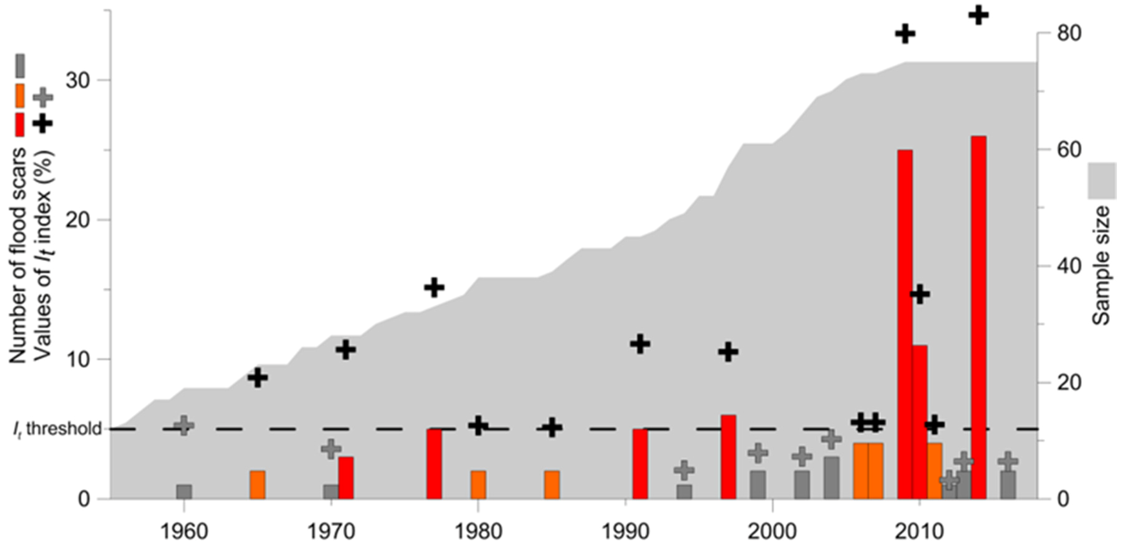
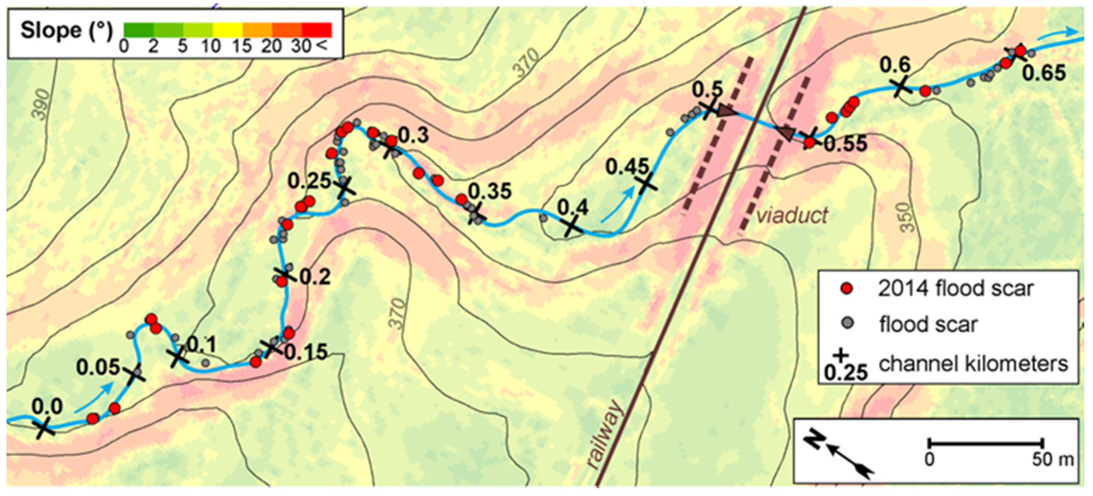
3.1. Chronology of Past Flood Events and Botanical Evidence of the May 2014 Flash Flood Event

In total, we successfully sampled and dated 75 scarred individuals (20 tree stems and 55 scarred roots) with a predominance of samples from P. sylvestris (37.3%), P. abies (18.7%), and A. glutinosa (17.3%), whereas five samples (root cross sections) had to be excluded from the chronology due to uncertainties during the dating procedure (Table 1). Eventually, it was possible to date 115 scars (1.5 scars per tree). Overall, we determined 13 flood events (seven certain and six probable events) during the period of 1955 to 2018 (limited by the minimum number of 10 sampled trees; Figure 4). The oldest (probable) event was recorded in 1965. The strongest signals (i.e., the highest value of the It index) were identified during 2014 (26 scars; It = 34.7%), 2009 (25 scars; It = 33.3%), and 1977 (5 scars; It = 15.2%).
Focusing on the botanical evidence of the 2014 flood event, we identified 26 scars throughout the whole study reach (6 scars on tree stems and 20 scars on exposed roots; Table 1). The mean height of the scars above the thalweg was 96.6 ± 34.6 cm. The minimum height (41 cm) was observed at 0.33 r. km at a straight channel reach, while the maximum height (156 cm) was recorded at 0.07 r. km at the failure of a concave bank. The distribution of the 2014 scars (Figure 5) was zero at the reach between 0.35 and 0.5 r. km, where the total number of scarred trees was generally lower, and the scars were generally of older dates. In contrast, the highest abundance of the 2014 flood scars was recorded between 0.2 and 0.35 r. km (11 scars overall).

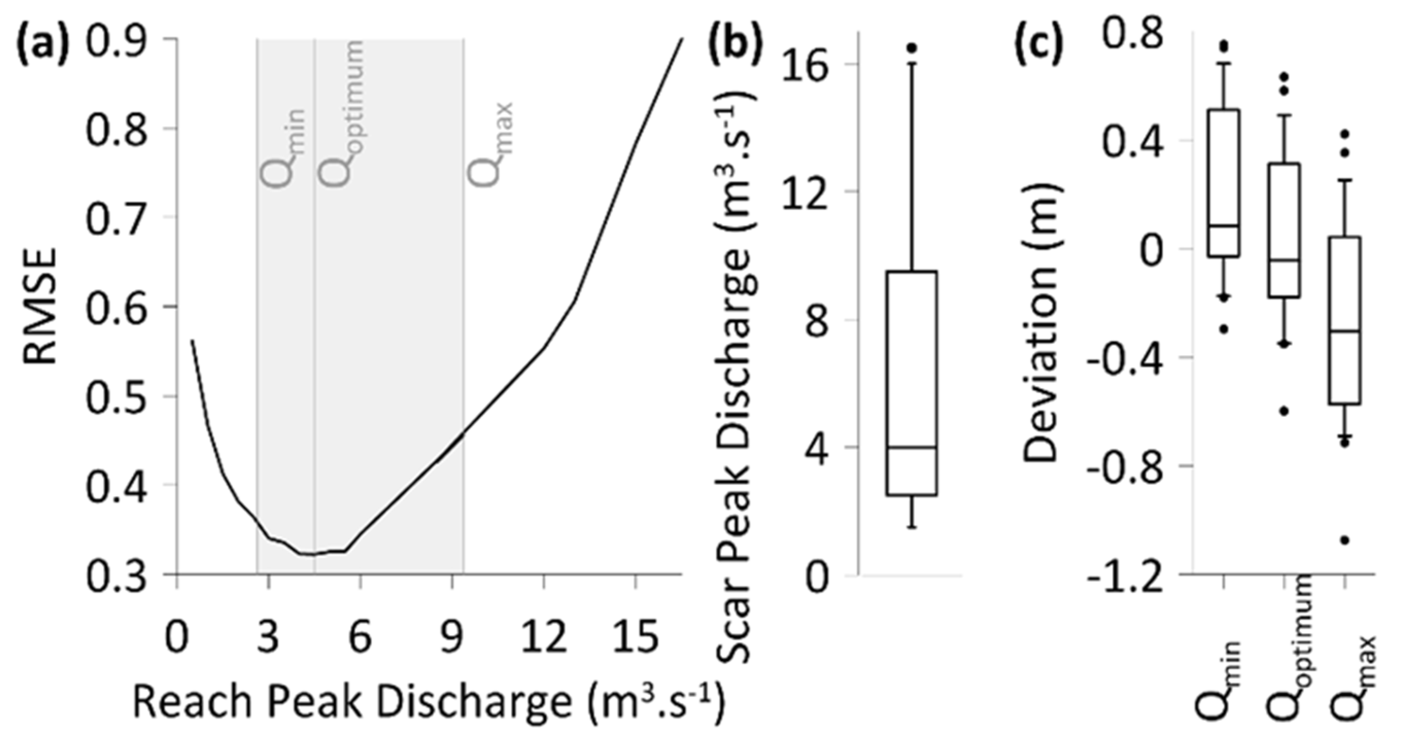
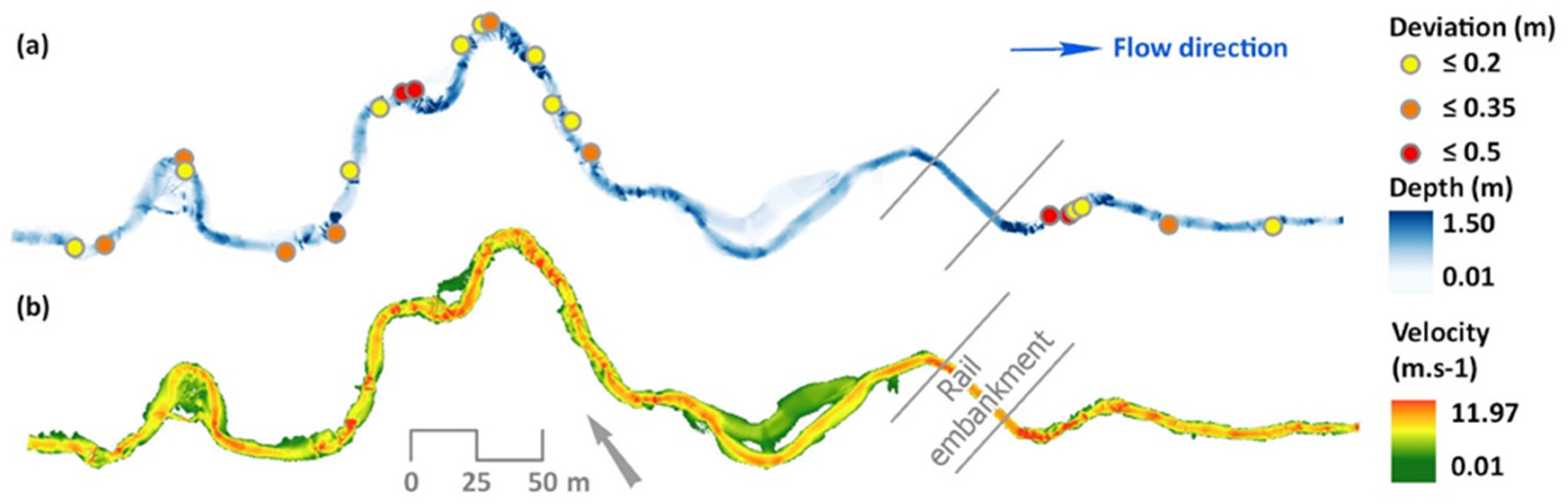
3.2. Results of Hydraulic Modelling

The flow conditions during the simulations were subcritical in the major part of the reach (91–94% of the total area) for all simulated flow scenarios (Table 2). Other flow characteristics (depth, velocity, and Froude number) resulting from the raster of hydraulic modelling are described in Table 2.
The characteristics of the RMSE curve of Qoptimum during the 2014 flood and the SPD characteristics are shown in Figure 6. The value of the reach peak discharge (Qoptimum) of the 2014 flood estimated by the RMSE (0.32 m) was equal to 4.5 m3·s−1. The values of the SPD showed high variability (coefficient of variability = 0.79) when the minimal SPD was 1.5 m3·s−1 and the maximal SPD was equal to 16.5 m3·s−1. The values of the Qmin and Qmax scenarios were calculated from all estimated SPD and were equal to 2.63 and 9.38 m3·s−1, respectively. The deviation between the measured PSI elevations and the simulated water level for Qoptimum ranged from −0.60 to 0.63 m with a median equal to −0.05 m. Similarly, the Qmin deviations ranged from −0.30 to 0.75 m, and the median was equal to 0.08 m. For Qmax, we registered deviations from −1.07 to 0.42 m, and the median was equal to −0.31 m. The highest magnitudes of velocity (up to 11.97 m·s−1; Figure 7) and bed shear stress (up to 1787.10 N.m−2) were registered at the positions of the highest changes in riverbed topography.
We further investigated the effect of the hydraulic conditions in the positions of the PSIs using non-parametric Spearman’s correlation. However, we did not observe any significant relationship between the PSI deviations and the velocity magnitudes for all three scenarios: Qoptimum (rsp = 0.19, p = 0.36), Qmin (rsp = 0.08; p = 0.71), and Qmax (rsp = 0.004; p = 0.98; Figure 8).

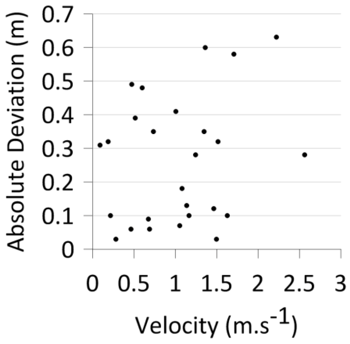
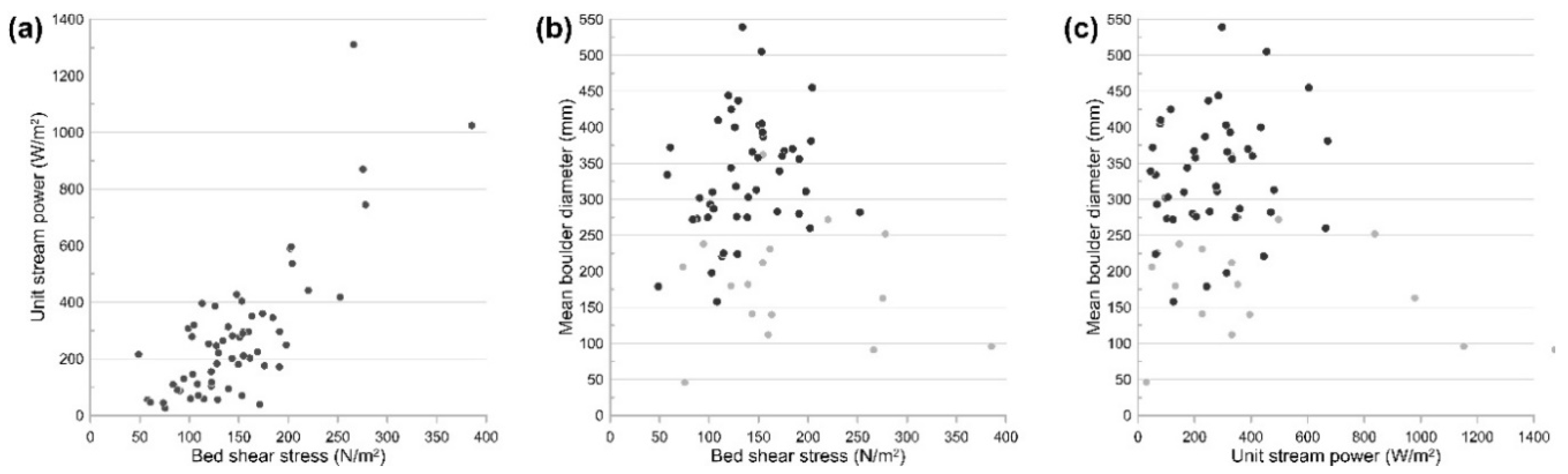
3.3. Channel Stability and Relations between the Hydraulic and Sedimentologic Parameters

A positive significant relationship exists between the bed shear stress and the unit stream power calculated for all cross sections (n = 62) and the Qoptimum scenario during the 2014 event (rsp = 0.65, p < 0.0001) (Figure 9a). In contrast, there were no significant correlations between the parameters of τb and MBD (rsp = 0.05, p = 0.68) or ω and MBD (rsp = −0.04, p = 0.74) (Figure 9b,c). After the removal of 15 cross-sections assigned to deep pools or bedrock sections containing a limited number of coarse grains, the final relationship was significant for τb and MBD (rsp = 0.33, p = 0.024) and remained insignificant for ω and MBD (rsp = 0.13, p = 0.38).
The mutual comparison of the MBD of cross sections located in depositional (n = 8), stable (n = 30) and erosional reaches (n = 24) showed significant differences between the groups (p = 0.002), when the cross sections of stable reaches indicated significantly higher values of MBD than those of locations with contemporary signs of prevailing depositional or erosional processes (Figure 10a). The analysis of the bed shear stress revealed significant differences between these groups (p = 0.012) when the cross sections of erosional reaches indicated significantly higher values of τb than those of the other groups (Figure 10b). On the other hand, we observed no significant differences among these groups in terms of ω (p = 0.095), although the erosional reaches were again characterised by somewhat higher values of ω than the other reaches (Figure 10c).
The evaluation of flow competence and the potential stability of coarse bed material in individual cross sections during the 2014 event showed that 15 of 62 cross sections (24.2%) indicated ωE ≥1 for the Qoptimum scenario (Figure 11). These cross sections were frequently representative of bedrock reaches with erosional tendencies with relatively fine grain-size character of the limited alluvial cover. An extraordinarily high excess was observed immediately downstream of the culvert (0.56–0.57 r. km). For the Qmax scenario, half of the cross sections (31 of 62; 50.0%) were perceived as those with unstable alluvial cover, still leaving the part upstream of the culvert (0.38–0.48 r. km) as relatively stable. On the other hand, the Qmin scenario predicted only seven unstable cross sections (11.3%) with a notable excess of critical unit stream power immediately downstream of the culvert (0.56–0.57 r. km).

4. Discussion

The dating of flood events, together with the determination of the 2014 flash flood parameters in the moderate relief of Central Europe, were introduced using the combination of dendrogeomorphic methods, 2D hydraulic modelling, and sedimentological parameters. Based on these approaches, we provide a quantitative estimation of the last flash flood event and a determination of channel reaches that tended to be (un)stable. Unlike the palaeoflood reconstructions from larger catchments, we included scarred roots as a possible PSI in the first-order catchments due to the generally lower peak flow discharges and lower volume of transported sediments. If the scarred root is a part of a stable root system and does not evidence a high rate of flexibility, it can be used not only as a helpful tool to date the time of (flood) erosion [21,60,61], but also as a PSI of recent floods.

4.1. Hydrogeomorphic Response of Flash Floods in the First-Order Catchment

The dendrogeomorphic results confirm that, despite the strong geomorphic impact of the last 2014 flash flood, there is evidence of former flood events within this catchment. We recorded the hydrogeomorphic impacts of floods in years with the occurrence of debris flows and rockfalls in the surrounding mountains (e.g., in 1991, 2006 and 2010 [62,63]). In addition, several identified years coincided with documentary data about local and/or regional flooding there (e.g., in 1971, 1977, 1997 and 2009). Polách and Gába [43] described a spatially limited downpour in July 1971 after strong antecedent precipitation, resulting in local damage to small streams within this region. This situation was likely similar to that of the last 2014 flash flood, which was considered unprecedented regarding the rainfall intensity, but the hydrogeomorphic response seems to be comparable to that of the 1971 event. Moreover, the transported parts of damaged culverts within the channel and several older scars on tree stems (Figure 2d) suggest an even higher hydrogeomorphic impact in the past. Furthermore, we identified that more than 40% of scars can be dated to the period 1951–2000, pointing to slow and progressive channel bank erosion during several flood events rather than to abrupt changes in channel geometry and the fast decay of exposed roots, as is typical for mountain regions [64].
We found no significant correlation by plotting the MBD and τb for all 62 cross sections, but a significant positive relationship existed after removal of fifteen cross sections assigned to deep pools and bedrock segments. This increase in statistical significance reflected the presence of the fine-grained character of the alluvial cover in these cross sections, the calibre of which did not necessarily correspond to the stream transport capacity (expressed by τb) during the examined flood event. Thus, we assumed more frequent transport of these fine particles during lower-magnitude events (e.g., bankfull or even lower flows). On the other hand, the set of remaining 47 cross sections had adjusted the calibre of the MBD to the calculated bed shear stresses. This positive relationship clearly pointed to the adjustment of the stepped-bed architecture during high-magnitude events towards a condition that provides the maximum possible bed stability, as was documented by previous flume experiments [65].
In general, the highest values of τb and ω were calculated for cross sections with erosional tendencies when compared to those of stable or depositional cross sections, although only the parameter of τb indicated statistically significant differences. These high values of τb and ω typically reflected a low width–depth ratio in erosional reaches with limited inundation ability together with the concentrated energy of flood flows. The presence of alluvial pockets of relatively fine sediments in the erosional reaches with exposed bedrock (resulting in very low values of MBD) explained our observations of the coarser bed particles in the stable reaches when one may expect local coarsening in erosional reaches with the highest calculated τb and, contrarily, fining in depositional reaches [23,66,67]. In addition, no differences in the MBD were observed between the erosional and stable reaches in the case of stepped-bed headwater streams based in flysch rocks, despite higher unit stream power being calculated for the erosional reaches [23]. These observations from small streams contradict the relation between the sediment coarsening and channel incision that was reported for gravel-bed rivers [68] by taking into consideration the specifics of steep headwater streams (e.g., mixture of alluvial and semi-alluvial reaches or strong effect of local lithology predicting patterns of sediment supply).
The parameter ω is frequently used to determine the capacity of a stream to mobilize specific bed grain sizes [37,69,70]. In our case, the excess critical unit stream power ωE identified the segments with unstable alluvial cover during the examined flood event. Only one-quarter of the cross sections indicated transport of the MBD under the Qoptimum scenario, when these cross sections were often representative of bedrock reaches with limited alluvial cover consisting of relatively fine grains. Even by applying the Qmax scenario, approximately 50% of the cross sections remained stable. Despite the large number of scars possibly related to intensive sediment transport and bank erosion during the 2014 flood, this event likely did not reach the critical threshold discharge to completely rework the stepped-bed character of the studied stream. Previous field measurements in steep mountain streams have perceived high-magnitude floods of up to a 50-year recurrence interval as those that mobilize most step-forming particles [71,72]. This suggests either a lower-than-expected magnitude of the 2014 flood described by local authorities or high channel bed stability of this first-order stream owing to the presence of large interlocked boulders.

4.2. Benefits and Limits of the Approach Used in the First-Order Catchment

Introducing the scarred roots as a PSI in a first-order catchment entails uncertainties similar to those in the case of scars on tree stems in larger rivers. As noted by several authors [18,36], PSIs located in straight channel reaches or on the inner side of channel bends are more suitable for peak discharge reconstructions than those of trees located on the outer side of channel bends or growing in overbank sections with dense vegetation cover. In our study, the majority of the PSIs (20) were located in the straight channel and/or inner side, reducing the overestimation of peak flow discharge. Moreover, the avoidance of root sampling in concave banks and slope failures for the PSI estimation reduces the probability of dating scars caused by bank/slope erosion. This situation may frequently occur, even during floods [73], but cannot be used as information about peak flow discharge.
A tricky situation may occur when several consecutive intense rainfalls affect the catchment. Therefore, more than one peak flow discharge may occur and thus enter as the uncertainty in hydraulic modelling. In our case, several storms generated during May 2014 could result in higher-than-average discharges [38], so we cannot exclude the possibility that several of the dated scars with lower PSI belong to some lower spring peak flows rather than to the surveyed flood of 27 May 2014. In contrast, anatomical analysis of some scarred roots revealed the position of the 2014 scar within the earlywood cells, pointing to the spring floods (Figure 3d) and thus eliminating the possible inclusion of scars during intense summer or autumn rainfall in 2014.
The results of the peak flow estimations show a high variation in SPD and high deviation in differences between the predicted water level and the observed PSI height. We hypothesize that this could be related to the small size of the catchment, where the role of the input data (PSI, DTM and roughness coefficient) is more crucial than in a large catchment (which produces large peak discharges). Similarly, Ballesteros-Cánovas et al. [18] reported the highest deviation of the estimated peak discharge in a catchment of the lowest size, while the opposite conclusions are described by Ballesteros-Cánovas et al. [57], where the authors reported much larger uncertainties for larger catchments than for smaller catchments. Following the approach of Bohorquez et al. [32], who defined the critical value of deviation between the simulated water level and the observed height of PSI as 0.2 m, for the Qmin, fifteen scars were within this range, followed by Qoptimum (12 PSI) and Qmax (10 PSI).
Further uncertainties associated with peak discharge reconstruction using the hydraulic model are related to the DTM accuracy [58] and model calibration. Although we tried to create an accurate DTM, especially at the position and close surroundings of the PSIs, our DTM is not error free, particularly between the cross sections where the interpolation took place. Victoriano et al. [34] found a 7% difference in the estimated peak discharge of 316 m3·s−1 (catchment area: 5.72 km2) when two different DTMs were compared. We call for further research to assess how the level of DTM accuracy influences the results of peak discharge reconstructions, even in small catchments. The uniform value of Manning’s roughness coefficient was applied over the overall reach, and the final value was a product of the calibration exercise to single “low-flow” discharge. Indeed, differences in the calibration for the low- and high-flow discharges are well known [56] and the influence of various values of Manning’s roughness coefficient on the results of the hydraulic model are described by Ballesteros-Cánovas et al. [57]. In fact, the hydraulic modelling of flood waves in large, low gradient rivers could cause serious problems with the approach used in this study (i.e., calibration to the discharge several orders of magnitude lower than simulated flood). However, in the case of small, high-gradient streams, this approach is better than the selection of the roughness value from the literature. Overall, we believe our approach reduced the uncertainty in the roughness coefficient to an acceptable level.
Although we considered the channel bed as a stable component with limited erosion and/or deposition during the 2014 flood, this does not reflect the natural condition in the modelled reach, because the majority of the riverbed is formed by poorly sorted alluvium with stripes of bedrock in a few places. This simplification could further influence the height of the PSI and the estimated discharge [14]. In addition, we did not observe any significant relationship between the velocity of the flood wave and the absolute deviation of the PSI from the modelled discharges (Qmin, Qoptimum, and Qmax), which is in agreement with the study of Ballesteros-Cánovas et al. [14]. We assume that the position of the PSI regarding the channel geometry (convex/concave/straight reach) is more important in small streams where the velocity is primarily changing with the stream gradient and channel width. Unfortunately, we were not able to test the influence of PSI deviations among convex, concave, and straight reaches due to the limited number of PSIs in each group.
We simulated subcritical flow over the overall reach, although supercritical flow occurred during the modelling in some parts. Flow conditions in steep channels can be transitional, with supercritical flow over the steps and subcritical flow in the pools. However, flow will never be supercritical throughout the simulated domain, because such flow would destabilize most channels [74]. This fact is supported by other studies [75,76], which described that, despite high velocity and extreme turbulence, flow in mountain streams is critical or subcritical, leading to the assumption that supercritical flow in natural streams does not exist for any extended length.

5. Conclusions

The estimations of peak flood discharges and the quantifications of related morphological changes and bedload transport in small streams remain a challenge, especially in the case of poorly gauged first-order catchments, despite their ability to transfer high amounts of water and sediment into low-order catchments. In this study, we presented an integrated approach based on palaeoflood reconstruction, which was performed in a first-order catchment in the moderate relief of Central Europe, to provide quantitative data about the last 2014 flash flood event and to create the chronology of former floods. The dendrogeomorphic results show the regular occurrence of flood events during at least the last 60 years, although the intensity of the last 2014 flash flood was considered to be unprecedented according to local authorities. The results of 2D hydraulic modelling are in favour of the optimum scenario of the 2014 peak flow discharge of 4.5 m3·s−1, which resulted in the formation of root and stem scars. Nevertheless, a sedimentological survey confirms the rather progressive development of the studied channel reach with limited ability to transport step-forming boulders during peak flow discharges similar to that in 2014 and thus relative bed stability during events of such magnitude. Despite notable geomorphic imprints and ongoing lateral erosion caused by the most recent flash flood events, with damage to infrastructure (especially in 2009 and 2014), we conclude that substantial geomorphic transition is practically excluded during the similar rainfall episodes that occurred within the last 60 years. The limited precision of the results of hydraulic modelling lead to the relatively high variability in possible peak flow in 2014 (from modelled Qmin to Qmax). This level of accuracy is still comparable to larger rivers, but may slightly change the interpretation of suggested event magnitudes in the case of smaller catchments. Therefore, further research dealing with the quality of input data into palaeoflood reconstruction (e.g., DTM accuracy and variable channel roughness) is crucial to investigation into first-order catchments.

Author Contributions

Conceptualization, R.T., S.R. and T.G.; methodology, R.T., S.R. and T.G.; validation, R.T., S.R. and T.G.; formal analysis, R.T., S.R. and T.G.; investigation, R.T., S.R. and T.G.; writing—original draft preparation, R.T., S.R. and T.G.; writing—review and editing, R.T.; visualization, R.T., S.R. and T.G. All authors have read and agreed to the published version of the manuscript.

Funding

This research received no external funding.

Acknowledgments

This research was supported by the University of Ostrava grant no. SGS02/PřF/2019–2020 “Quaternary development and contemporary state of Central European landscape in the context of geohazard action, effects of anthropopressure, and climate changes”. Jakub Hrubý and Ondřej Vala are acknowledged for their help during fieldworks. English language was edited by American Journal Experts.

Conflicts of Interest

The authors declare no conflict of interest.

References

  1. Baker, V.R. Geomorphological understanding of floods. In Geomorphology and Natural Hazards, 1st ed.; Morisawa, M., Ed.; Elsevier: Amsterdam, The Netherlands, 1994; pp. 139–156. [Google Scholar] [CrossRef]
  2. Jakob, M.; Hungr, O. Debris-Flow Hazards and Related Phenomena; Springer: Berlin, Germany, 2005; p. 781. [Google Scholar] [CrossRef]
  3. Petrow, T.; Merz, B. Trends in flood magnitude, frequency and seasonality in Germany in the period 1951–2002. J. Hydrol. 2009, 371, 129–141. [Google Scholar] [CrossRef] [Green Version]
  4. Amponsah, W.; Marchi, L.; Zoccatelli, D.; Boni, G.; Cavalli, M.; Comiti, F.; Crema, S.; Lucia, A.; Marra, F.; Borga, M. Hydrometeorological characterization of a flash flood associated with major geomorphic effects: Assessment of peak discharge uncertainties and analysis of the runoff response. J. Hydrometeorol. 2016, 17, 3063–3077. [Google Scholar] [CrossRef]
  5. Saharia, M.; Kirstetter, P.E.; Vergara, H.; Gourley, J.J.; Hong, Y. Characterization of floods in the United States. J. Hydrol. 2017, 548, 524–535. [Google Scholar] [CrossRef]
  6. Strahler, A.N. Quantitative analysis of watershed geomorphology. Trans. Am. Geophys. Union 1957, 38, 913–920. [Google Scholar] [CrossRef] [Green Version]
  7. Raška, P.; Brázdil, R. Participatory responses to historical flash floods and their relevance for current risk reduction: A view from a post-communist country. Area 2015, 47, 166–178. [Google Scholar] [CrossRef]
  8. Fuchs, S.; Heiss, K.; Hübl, J. Towards an empirical vulnerability function for use in debris flow risk assessment. Nat. Hazards Earth Syst. Sci. 2007, 7, 495–506. [Google Scholar] [CrossRef] [Green Version]
  9. Ballesteros-Cánovas, J.A.; Stoffel, M.; Corona, C.; Schraml, K.; Gobiet, A.; Tani, S.; Sinabell, F.; Fuchs, S.; Kaitna, R. Debris-flow risk analysis in a managed torrent based on a stochastic life-cycle performance. Sci. Total Environ. 2016, 557, 142–153. [Google Scholar] [CrossRef]
  10. Ozturk, U.; Wendi, D.; Crisologo, I.; Riemer, A.; Agarwal, A.; Vogel, K.; López-Tarazón, J.A.; Korup, O. Rare flash floods and debris flows in southern Germany. Sci. Total Environ. 2018, 626, 941–952. [Google Scholar] [CrossRef]
  11. Terti, G.; Ruin, I.; Anquetin, S.; Gourley, J.J. Dynamic vulnerability factors for impact-based flash flood prediction. Nat. Hazards 2015, 79, 1481–1497. [Google Scholar] [CrossRef]
  12. Alestalo, J. Dendrochronological interpretation of geomorphic processes. Fennia 1971, 105, 1–140. [Google Scholar]
  13. Stoffel, M.; Bollschweiler, M. Tree-ring analysis in natural hazards research? An overview. Nat. Hazards Earth Syst. Sci. 2008, 8, 187–202. [Google Scholar] [CrossRef] [Green Version]
  14. Ballesteros-Cánovas, J.A.; Eguibar, M.; Bodoque, J.M.; Díez-Herrero, A.; Stoffel, M.; Gutiérrez-Pérez, I. Estimating flash flood discharge in an ungauged mountain catchment with 2D hydraulic models and dendrogeomorphic palaeostage indicators. Hydrol. Process. 2011, 25, 970–979. [Google Scholar] [CrossRef] [Green Version]
  15. Garrote, J.; Díez-Herrero, A.; Bodoque, J.M.; Perucha, M.A.; Mayer, P.L.; Génova, M. Flood hazard management in public mountain recreation areas vs. ungauged fluvial basins. Case study of the Caldera de Taburiente National Park, Canary Islands (Spain). Geosciences 2018, 8, 6. [Google Scholar] [CrossRef] [Green Version]
  16. Gottesfeld, A.S. British Columbia flood scars: maximum flood-stage indicators. Geomorphology 1996, 14, 319–325. [Google Scholar] [CrossRef]
  17. Yanosky, T.M.; Jarrett, R.D. Dendrochronologic evidence for the frequency and magnitude of paleofloods. In Ancient Floods, Modern Hazards: Principles and Applications of Paleoflood Hydrology; House, P.K., Webb, R.H., Baker, V.R., Levish, D.R., Eds.; American Geophysical Union: Washington, DC, USA, 2002; Volume 5, pp. 77–89. [Google Scholar]
  18. Ballesteros-Cánovas, J.A.; Stoffel, M.; Spyt, B.; Janecka, K.; Kaczka, R.J.; Lempa, M. Paleoflood discharge reconstruction in Tatra Mountain streams. Geomorphology 2016, 272, 92–101. [Google Scholar] [CrossRef]
  19. Ballesteros-Cánovas, J.A.; Trappmann, D.; Shekhar, M.; Bhattacharyya, A.; Stoffel, M. Regional flood-frequency reconstruction for Kullu district, Western Indian Himalayas. J. Hydrol. 2017, 546, 140–149. [Google Scholar] [CrossRef]
  20. McCord, V.A. Fluvial process dendrogeomorphology: Reconstruction of flood events from the southwestern United States using flood-scarred trees. In Tree Rings, Environment and Humanity; Dean, J.S., Meko, D.M., Swetnam, T.W., Eds.; Radiocarbon Department of Geosciences University of Arizona: Tucson, AZ, USA, 1996; pp. 689–699. [Google Scholar]
  21. Stoffel, M.; Casteller, A.; Luckman, B.H.; Villalba, R. Spatiotemporal analysis of channel wall erosion in ephemeral torrents using tree roots—An example from the Patagonian Andes. Geology 2012, 40, 247–250. [Google Scholar] [CrossRef]
  22. Chappell, P.R.; Brierley, G.J. Multi-scalar controls on channel geometry of headwater streams in New Zealand hill country. Catena 2014, 113, 341–352. [Google Scholar] [CrossRef]
  23. Galia, T.; Škarpich, V. Do the coarsest bed fractions and stream power record contemporary trends in steep headwater channels? Geomorphology 2016, 272, 115–126. [Google Scholar] [CrossRef]
  24. Harvey, A.M. Coupling between hillslopes and channels in upland fluvial systems: Implications for landscape sensitivity, illustrated from the Howgill Fells, northwest England. Catena 2001, 42, 225–250. [Google Scholar] [CrossRef]
  25. Kavage Adams, R.; Spotila, J.A. The form and function of headwater streams based on field and modeling investigations in the Southern Appalachian Mountains. Earth Surf. Process. Landf. 2005, 30, 1521–1546. [Google Scholar] [CrossRef] [Green Version]
  26. May, C.L.; Gresswell, R.E. Processes and rates of sediment and wood accumulation in headwater streams of the Oregon Coast Range, USA. Earth Surf. Process. Landf. 2003, 28, 409–424. [Google Scholar] [CrossRef]
  27. Comiti, F.; Mao, L. Recent advances in the dynamics of steep channels. In Gravel-Bed Rivers: Processes, Tools, Environments; Church, M., Biron, P.M., Roy, A.G., Eds.; John Wiley & Sons: Hoboken, NJ, USA, 2012; pp. 351–377. [Google Scholar] [CrossRef]
  28. Bunte, K.; Abt, S.R.; Swingle, K.W.; Cenderelli, D.A. Effective discharge in Rocky Mountain headwater streams. J. Hydrol. 2014, 519, 2136–2147. [Google Scholar] [CrossRef]
  29. Lenzi, M.A.; Mao, L.; Comiti, F. Effective discharge for sediment transport in a mountain river: Computational approaches and geomorphic effectiveness. J. Hydrol. 2006, 326, 257–276. [Google Scholar] [CrossRef]
  30. Lenzi, M.A.; Mao, L.; Comiti, F. When does bedload transport begin in steep boulder-bed streams? Hydrol. Process. 2006, 20, 3517–3533. [Google Scholar] [CrossRef]
  31. Chiari, M.; Rickenmann, D. Back-calculation of bedload transport in steep channels with a numerical model. Earth Surf. Process. Landf. 2011, 36, 805–815. [Google Scholar] [CrossRef]
  32. Bohorquez, P.; Daby, S.E. The use of one- and two-dimensional hydraulic modelling to reconstruct a glacial outburst flood in a steep Alpine valley. J. Hydrol. 2008, 341, 240–261. [Google Scholar] [CrossRef] [Green Version]
  33. Ruiz-Villanueva, V.; Díez-Herrero, A.; Bodoque, J.M.; Ballesteros-Cánovas, J.A.; Stoffel, M. Characterisation of flash floods in small ungauged mountain basins of Central Spain using an integrated approach. Catena 2013, 110, 32–43. [Google Scholar] [CrossRef]
  34. Victoriano, A.; Díez-Herrero, A.; Génova, M.; Guinau, M.; Furdada, G.; Khazaradze, G.; Calvet, J. Four-topic correlation between flood dendrogeomorphological evidence and hydraulic parameters (the Portainé stream, Iberian Peninsula). Catena 2018, 162, 216–229. [Google Scholar] [CrossRef]
  35. Balasch, J.C.; Pino, D.; Ruiz-Bellet, J.L.; Tuset, J.; Barriendos, M.; Castelltort, X.; Peña, J.C. The extreme floods in the Ebro River basin since 1600 CE. Sci. Total Environ. 2019, 646, 645–660. [Google Scholar] [CrossRef]
  36. Bodoque, J.M.; Díez-Herrero, A.; Eguibar, M.A.; Benito, G.; Ruiz-Villanueva, V.; Ballesteros-Cánovas, J.A. Challenges in paleoflood hydrology applied to risk analysis in mountainous watersheds—A review. J. Hydrol. 2015, 529, 449–467. [Google Scholar] [CrossRef] [Green Version]
  37. Mao, L.; Uyttendaele, G.P.; Iroumé, A.; Lenzi, M.A. Field based analysis of sediment entrainment in two high gradient streams located in Alpine and Andine environments. Geomorphology 2008, 93, 368–383. [Google Scholar] [CrossRef]
  38. Tichavský, R.; Kluzová, O.; Břežný, M.; Ondráčková, L.; Krpec, P.; Tolasz, R.; Šilhán, K. Increased gully activity induced by short-term human interventions—Dendrogeomorphic research based on exposed tree roots. Appl. Geogr. 2018, 98, 66–77. [Google Scholar] [CrossRef]
  39. Povodí Odry. Zpráva o Povodni Květen 2014 v Dílčím Povodí Horní Odry; Povodí Odry, Státní Podnik: Ostrava, Czech Republic, 2014; p. 34. (In Czech) [Google Scholar]
  40. Cháb, J.; Čurda, J.; Kočandrle, J.; Manová, M.; Nývlt, D.; Pecina, V.; Skácelová, D.; Večeřa, J.; Žáček, V. Základní Geologická Mapa České Republiky 1: 25000, List 14–224 Jeseník s Textovými Vysvětlivkami; Česká Geologická Služba: Prague, Czech Republic, 2004; p. 75. (In Czech) [Google Scholar]
  41. Hanáček, M.; Nývlt, D.; Skácelová, Z.; Nehyba, S.; Procházková, B.; Engel, Z. Sedimentary evidence for an ice-sheet dammed lake in a mountain valley of the Eastern Sudetes, Czechia. Acta Geol. Pol. 2018, 68, 107–134. [Google Scholar]
  42. Tolasz, R.; Brázdil, R.; Bulíř, O.; Dobrovolný, P.; Hájková, L.; Halásová, O.; Hostýnek, J.; Janouch, M.; Kohut, M.; Krška, K.; et al. Atlas Podnebí ČR, 1st ed.; Czech Hydrometeorological Institute/Palacky University: Praha, Czech Republic; Olomouc, Czech Republic, 2007; p. 256. (In Czech) [Google Scholar]
  43. Polách, D.; Gába, Z. Historie povodní na šumperském a jesenickém okrese. Severní Morava 1998, 75, 3–28. (In Czech) [Google Scholar]
  44. Ballesteros-Cánovas, J.A.; Stoffel, M.; St George, S.; Hirschboeck, K. A review of flood records from tree rings. Prog. Phys. Geogr. 2015, 39, 794–816. [Google Scholar] [CrossRef]
  45. Ballesteros-Cánovas, J.A.; Márquez-Peñaranda, J.F.; Sánchez-Silva, M.; Díez-Herrero, A.; Ruiz-Villanueva, V.; Bodoque, J.M.; Eguibar, M.A.; Stoffel, M. Can tree tilting be used for paleoflood discharge estimations? J. Hydrol. 2015, 529, 480–489. [Google Scholar] [CrossRef]
  46. Bräker, O.U. Measuring and data processing in tree-ring research—A methodological introduction. Dendrochronologia 2002, 20, 203–216. [Google Scholar] [CrossRef]
  47. Vienna Institute of Archaeological Science (VIAS). Time Table. Installation and Instruction Manual; Version 2.1; University of Vienna: Vienna, Austria, 2005. [Google Scholar]
  48. Holmes, R.L.; Adams, R.K.; Fritts, H.C. Tree-Ring Chronologies of Western North America: California, Eastern Oregon and Northern Great Basin with Procedures Used in the Chronology Development Work Including Users Manuals for Computer Programs COFECHA and ARSTAN; Laboratory of Tree-Ring Research, University of Arizona: Tucson, AZ, USA, 1986; p. 182. [Google Scholar]
  49. Wrońska-Wałach, D.; Sobucki, M.; Buchwał, A.; Gorczyca, E.; Korpak, J.; Wałdykowski, P.; Gärtner, H. Quantitative analysis of ring growth in spruce roots and its application towards a more precise dating. Dendrochronologia 2016, 38, 61–71. [Google Scholar] [CrossRef]
  50. Gärtner, H.; Lucchinetti, S.; Schweingruber, F.H. A new sledge microtome to combine wood anatomy and tree-ring ecology. IAWA J. 2015, 36, 452–459. [Google Scholar] [CrossRef]
  51. Gärtner, H.; Cherubini, P.; Fonti, P.; von Arx, G.; Schneider, L.; Nievergelt, D.; Verstege, A.; Bast, A.; Schweingruber, F.H.; Büntgen, U. A Technical Perspective in Modern Tree-ring Research—How to Overcome Dendroecological and Wood Anatomical Challenges. J. Vis. Exp. 2015, 97, e52337. [Google Scholar] [CrossRef] [Green Version]
  52. Shroder, J.F. Dendrogeomorphological analysis of mass movement on Table Cliffs Plateau, Utah. Quat. Res. 1978, 9, 168–185. [Google Scholar] [CrossRef]
  53. Bladé, E.; Cea, L.; Corestein, G.; Escolano, E.; Puertas, J.; Vázquez-Cendón, E.; Dolz, J.; Coll, A. Iber: Herramienta de simulación numérica del flujo en ríos. Revista Internacional de Métodos Numéricos para Cálculo y Diseño en Ingeniería 2014, 30, 1–10. [Google Scholar] [CrossRef] [Green Version]
  54. Webb, R.H.; Jarrett, R.D. One-dimensional estimation techniques for discharges of paleofloods and historical floods. In Ancient Floods, Modern Hazards: Principles and Applications of Paleoflood Hydrology; House, P.K., Webb, R.H., Baker, V.R., Levish, D.R., Eds.; American Geophysical Union: Washington, DC, USA, 2002; Volume 5, pp. 111–126. [Google Scholar]
  55. Yochum, S.E.; Bledsoe, B.P.; David, G.C.; Wohl, E. Velocity prediction in high-gradient channels. J. Hydrol. 2012, 424, 84–98. [Google Scholar] [CrossRef]
  56. Ferguson, R.I.; Sharma, B.P.; Hardy, R.J.; Hodge, R.A.; Warburton, J. Flow resistance and hydraulic geometry in contrasting reaches of a bedrock channel. Water Resour. Res. 2017, 53, 2278–2293. [Google Scholar] [CrossRef] [Green Version]
  57. Ballesteros-Cánovas, J.A.; Bodoque, J.M.; Díez-Herrero, A.; Sanchez-Silva, M.; Stoffel, M. Calibration of floodplain roughness and estimation of palaeoflood discharge based on tree-ring evidence and hydraulic modelling. J. Hydrol. 2011, 403, 103–115. [Google Scholar] [CrossRef]
  58. Casas, A.; Benito, G.; Thorndycraft, V.R.; Rico, M. The topographic data source of digital terrain models as a key element in the accuracy of hydraulic flood modelling. Earth Surf. Process. Landf. J. Br. Geomorphol. Res. Group 2006, 31, 444–456. [Google Scholar] [CrossRef]
  59. Galia, T.; Hradecký, J. Critical conditions for the beginning of coarse sediment transport in the torrents of the Moravskoslezské Beskydy Mts (Western Carpathians). Carpath. J. Earth Environ. Sci. 2012, 7, 5–14. [Google Scholar]
  60. Malik, I.; Matyja, M. Bank erosion history of a mountain stream determined by means of anatomical changes in exposed tree roots over the last 100 years (Bílá Opava River—Czech Republic). Geomorphology 2008, 98, 126–142. [Google Scholar] [CrossRef]
  61. Šilhán, K.; Galia, T. Sediment (un) balance budget in a high-gradient stream on flysch bedrock: A case study using dendrogeomorphic methods and bedload transport simulation. Catena 2015, 124, 18–27. [Google Scholar] [CrossRef]
  62. Tichavský, R.; Šilhán, K.; Tolasz, R. Tree ring-based chronology of hydro-geomorphic processes as a fundament for identification of hydro-meteorological triggers in the Hrubý Jeseník Mountains (Central Europe). Sci. Total Environ. 2017, 579, 1904–1917. [Google Scholar] [CrossRef] [PubMed]
  63. Lenart, J.; Tichavský, R.; Večeřa, J.; Kapustová, V.; Šilhán, K. Genesis and geomorphic evolution of the Velké pinky stopes in the Zlatohorská Highlands, Eastern Sudetes. Geomorphology 2017, 296, 91–103. [Google Scholar] [CrossRef]
  64. Tichavský, R. Unravelling the recent dynamics of headwaters based on a combined dendrogeomorphic approach (a case study from the Sudetes Mts., Czech Republic). Geogr. Ann. Ser. A Phys. Geogr. 2019, 101, 16–33. [Google Scholar] [CrossRef]
  65. Weichert, R.B.; Bezzola, G.R.; Minor, H.E. Bed morphology and generation of step-pool channels. Earth Surf. Process. Landf. J. Br. Geomorphol. Res. Group 2008, 33, 1678–1692. [Google Scholar] [CrossRef]
  66. Addy, S.; Soulsby, C.; Hartley, A.J.; Tetzlaff, D. Characterisation of channel reach morphology and associated controls in deglaciated montane catchments in the Cairngorms, Scotland. Geomorphology 2011, 132, 176–186. [Google Scholar] [CrossRef]
  67. Thompson, C.J.; Croke, J.; Ogden, R.; Wallbrink, P. A morpho-statistical classification of mountain stream reach types in southeastern Australia. Geomorphology 2006, 81, 43–65. [Google Scholar] [CrossRef]
  68. Zawiejska, J.; Wyżga, B.; Radecki-Pawlik, A. Variation in surface bed material along a mountain river modified by gravel extraction and channelization, the Czarny Dunajec, Polish Carpathians. Geomorphology 2015, 231, 353–366. [Google Scholar] [CrossRef]
  69. Gob, F.; Bravard, J.P.; Petit, F. The influence of sediment size, relative grain size and channel slope on initiation of sediment motion in boulder bed rivers. A lichenometric study. Earth Surf. Process. Landf. 2010, 35, 1535–1547. [Google Scholar] [CrossRef]
  70. Petit, F.; Gob, F.; Houbrechts, G.; Assani, A.A. Critical specific stream power in gravel-bed rivers. Geomorphology 2005, 69, 92–101. [Google Scholar] [CrossRef]
  71. Lenzi, M.A. Displacement and transport of marked pebbles, cobbles and boulders during floods in a steep mountain stream. Hydrol. Process. 2004, 18, 1899–1914. [Google Scholar] [CrossRef]
  72. Molnar, P.; Densmore, A.L.; McArdell, B.W.; Turowski, J.M.; Burlando, P. Analysis of changes in the step-pool morphology and channel profile of a steep mountain stream following a large flood. Geomorphology 2010, 124, 85–94. [Google Scholar] [CrossRef]
  73. Šilhán, K.; Galia, T.; Škarpich, V. Detailed spatio-temporal sediment supply reconstruction using tree roots data. Hydrol. Process. 2016, 30, 4139–4153. [Google Scholar] [CrossRef]
  74. Church, M.; Zimmermann, A. Form and stability of step-pool channels: Research progress. Water Resour. Res. 2007, 43, W03415. [Google Scholar] [CrossRef]
  75. Jarrett, R.D. Hydraulics of high-gradient streams. J. Hydraul. Eng. 1984, 110, 1519–1539. [Google Scholar] [CrossRef]
  76. Trieste, D.J. Evaluation of supercritical/subcritical flows in high-gradient channel. J. Hydraul. Eng. 1992, 118, 1107–1118. [Google Scholar] [CrossRef]
Figure 1. Location of the study site: position within Central Europe (a), within the Eastern Sudetes (b), and (c) orthophoto image of the studied catchment (1—study channel reach, 2—main road, 3—railway and 4—cycle path).
Water 12 00212 g001
Figure 2. Morphological features of the study channel reach: (a) channel bottom composed of gneiss bedrock; (b) channel widening evidenced by the system of exposed tree roots in boulder-step reach; (c) step-pool reach with the presence of channel widening and fresh, shallow slope failure; (d) flood scars (higher older, and lower younger) on the tree stem of A. glutinosa in the direction of flow (note the remnants of concrete parts of centring transported by past floods).
Water 12 00212 g002
Figure 3. Identified flood scars: (a) the 2014 flood scar on the root section of P. abies; (b) the 2009 flood scar on the root section of T. cordata; (c) the 2014 flood scar on the stem wedge of A. glutinosa; and (d) the 2014 flood scar on the root microsection of P. sylvestris, with the obvious position within earlywood cells indicating the flood event on 27 May.
Water 12 00212 g003
Figure 4. Number of identified flood scars and the final chronology of flood events (based on thresholds: It ≥ 5% and number of scars ≥ 2). The red column indicates a certain event, and the orange column indicates a probable event. The grey column and grey cross indicate years that could not be considered flood events.
Water 12 00212 g004
Figure 5. Localization of the 2014 flood scars within the studied channel reach.
Water 12 00212 g005
Figure 6. Parameters of the 2014 modelled flood discharge: (a) RMSE curve for the reach peak discharges where three scenarios are visualized with the uncertainty defined by Qmin and Qmax (filled rectangle); (b) the box plot of scar peak discharges; (c) the box plots of deviation between the measured PSI elevation and simulated water level. Whiskers in (b,c) are equal to the 10th and 90th percentiles (n = 26).
Water 12 00212 g006
Figure 7. Raster outputs of hydraulic modelling for the Qoptimum scenario: (a) water depth and (b) velocity. Colored circles illustrate the position of the 2014 PSI (scars) and deviations of their heights from the modelled flow.
Water 12 00212 g007
Figure 8. Plot describing the relationships between the flow velocity and absolute deviation of the PSI for Qoptimum scenario.
Water 12 00212 g008
Figure 9. Plots between (a) the bed shear stress and unit stream power, (b) the bed shear stress and mean boulder diameter, and (c) the unit stream power and mean boulder diameter. The grey points in plots (b,c) indicate cross sections located in bedrock reaches or deep pools.
Water 12 00212 g009
Figure 10. Boxplots of mean boulder diameter, bed shear stress and unit stream power calculated for the 2014 event (Qoptimum scenario) in erosional, stable and depositional cross sections. The letters above the boxes show significantly different groups by Z-value test with Bonferonni corrections.
Water 12 00212 g010
Figure 11. Downstream variations in the excess of critical unit stream power for the 2014 event (critical threshold 1 is indicated by the red dashed line) and dominant fluvial processes. The individual blue points represent values calculated for the Qoptimum scenario for individual cross sections; the scatter lines around these points indicate the values of the Qmin and Qmax scenarios. The occurrence of bedrock reaches is indicated by black rectangles marked by ‘b’ letters.
Water 12 00212 g011
Table 1. Overall number of sampled and dated trees and the distribution of samples containing the 2014 scar.
Tree SpeciesNr. of TreesPercentage of Trees (%)Nr. of Root SectionsNr. of Stem Sections/CoresNumber of Samples Containing the 2014 Scar
RootStem
Pinus sylvestris2837.328050
Picea abies1418.713160
Alnus incana1317.36742
Tilia cordata912.07240
Acer pseudoplatanus68.00602
Sorbus aucuparia56.71412
Total75100.05520206
Table 2. Selected flow characteristics for flow scenarios applied in this study.
Flow Characteristics/ScenarioDepth (m)Velocity (m·s−1)FroudeArea of Supercritical Flow (%)
MeanMaxMeanMaxMeanMax
Qmin0.351.411.059.430.593.676.43
Qoptimum0.431.501.1711.970.613.797.37
Qmax0.591.951.4412.020.643.889.01

