Long-Term Homogeneity, Trend, and Change-Point Analysis of Rainfall in the Arid District of Ananthapuramu, Andhra Pradesh State, India

Abstract

The objective of this study is to evaluate the homogeneity, trend, and trend change points in the rainfall data. Daily rainfall data was collected for the arid district of Ananthapuramu, Andhra Pradesh state, India from 1981 to 2016 at the subdistrict level and aggregated to monthly, annual, seasonal rainfall totals, and the number of rainy days. After quality checks and homogeneity analysis, a total of 27 rain gauge locations were considered for trend analysis. A serial correlation test was applied to all the time series to identify serially independent series. NonParametric Mann–Kendall test and Spearman’s rank correlation tests were applied to serially independent series. The magnitude of the trend was calculated using Sen’s slope method. For the data influenced by serial correlation, various modified versions of Mann–Kendall tests (pre-whitening, trend-free pre-whitening, bias-corrected pre-whitening, and two variants of variance correction approaches) were applied. A significant increasing summer rainfall trend is observed in six out of 27 stations. Significant decreasing trends are observed at two stations during the southwest monsoon season and at two stations during the northeast monsoon season. To identify the trend change points in the time series, distribution−free cumulative sum test, and sequential Mann–Kendall tests were applied. Two open−source library packages were developed in R language namely, ”modifiedmk” and ”trendchange” to implement the statistical tests mentioned in this paper. The study results benefit water resource management, drought mitigation, socio−economic development, and sustainable agricultural planning in the region.

1. Introduction

Hydrological regime is under a lot of stress due to climate change and is gaining a lot of attention in the scientific community due to its potential adverse effects on the environment [1]. Rainfall variability plays a major role in the Indian economy and extreme rainfall events resulting in drought and floods impact the nation’s food security and Gross Domestic Product (GDP) [2]. India is quite vulnerable to climate change and its impact on various sectors such as water resources, agriculture, forestry, and the health sector, etc. are well documented by several researchers [3,4,5,6,7,8,9,10]. Detailed analysis of rainfall trend is useful to rainfall forecasting, planning water resources development and management, designing water storage structures, irrigation practices and crop choices, drinking water supply, industrial development, and disaster management for current and future climatic conditions [11,12,13,14,15]. The evaluation of past trends of meteorological parameters at various spatial and temporal scales plays a crucial role in understanding climate change and its impact on food security, energy security, natural resource management, and sustainable development [16,17].

In order to represent true variations in the weather and climate, the assumption of homogeneity in meteorological observations is quite important in climatological trend analysis. The direct methods of homogenization involve best management practices in data recording and archiving. Indirect methods of homogenization involve metadata analysis, creation of reference series, statistical tests for breakpoint detection, and adjustment of the data records [18,19]. To identify the effects of non−climatic factors in the observations over time, homogeneity tests are performed on time series data. The homogeneity tests are of two types, namely absolute methods and relative methods. In the case of absolute homogeneity tests, each station is considered separately without considering the effect of neighboring stations. In relative homogeneity tests, neighboring reference stations are used. Several researchers have either assumed the data to be homogeneous or used absolute homogeneity tests alone in their research [20,21,22,23,24,25]. It has been suggested to use the relative homogeneity tests if the neighboring stations are within the same climatic region [26,27].

In the literature, researchers have used parametric and nonparametric methods of trend detection in time series data. Parametric trend tests assume the data to be random, independent, and normally distributed. Nonparametric trend tests are widely used in the literature as they do not assume any statistical distribution in the data [28,29,30,31,32,33]. However, the assumption of serial independence and randomness stands unchanged for nonparametric trend tests. Serial correlation affects the power of trend tests to identify trends correctly in the time series data [34,35]. The Mann–Kendall test (MK) [36,37], Spearman’s rank correlation coefficient test (SRC) [38,39] for trend detection, and Sen’s slope test (SS) for calculating trend magnitude [40,41] are perhaps the most widely used nonparametric tests in the previous studies. The power of the Mann–Kendall test and Spearman’s rho tests are positively affected by the sample size, magnitude of the trend, and significance level considered in the analysis; while it is negatively affected by time series variations [42].

A majority of previous studies have used the Mann–Kendall test for trend detection and Sen’s slope test to report trend magnitude in the case of serially independent data. To minimize the impact of serial correlation on trend detection, various methods such as pre-whitening (PW) [35,43], trend-free pre-whitening (TFPW) [44], bias-corrected pre-whitening (BCPW) [45], variance correction approach (VCA) [46,47], and block bootstrapping (BBS) [48,49], etc., have been proposed in literature. When the time series are serially correlated, researchers have either ignored it or used one of several modified versions of Mann–Kendall tests to report trends. It is recommended to use a combination of statistical tests in trend analysis at various confidence intervals [28,50]. It is very important to study the change point of the trend, along with trend analysis. Very few researchers have reported the time of trend change in their research [28].

The Ananthapuramu district is an arid agro-ecological region of India, which is highly vulnerable to climate change [51]. The Ananthapuramu region falls under Rayalaseema meteorological subdivision. Guhathakurta et al. [52] and Kaur et al. [53] analyzed rainfall trends at meteorological subdivisions using Indian Meteorological Department’s (IMD) rainfall data for the period from 1901 to 2003. The results from Guhathakurta et al. [52] indicated increasing annual and southwest monsoon rainfall and decreasing winter and northeast monsoon rainfall. Kaur et al. [53] reported increasing annual and southwest monsoon rainfall. Mondal et al. [54] reported a decreasing summer rainfall. Sivajothi et al. [55] used district-level average rainfall data and reported a significant increasing annual and northeast monsoon rainfall and a decreasing southwest monsoon rainfall. Naveen et al. [56] presented a detailed analysis of various climatological parameters such as rainfall, temperature, wind speed, humidity, evaporation, solar radiation, etc., of the Ananthapuramu district. Reddy et al. [57] presented a comprehensive study of drought conditions in the Ananthapuramu district. Rao et al. [58] investigated the trends in heavy rainfall events of the Ananthapuramu district using the rainfall data for the period from 1971 to 2008. This study is perhaps the first to report the rainfall trends in the Ananthapuramu district at the subdistrict level.

The entire district of Ananthapuramu is declared as a hot-arid zone and several watershed management programs have been initiated to mitigate the drought conditions. The majority of the farmers in the district are marginal or small farmers and are highly vulnerable to climate change. Climate resilient agriculture and best management practices in farming are required in the region for sustainable agriculture [59,60]. Groundwater quality is very alarming in many areas of the Ananthapuramu district, and the situation could worsen due to changes in the precipitation pattern [61].

The objective of this study is to investigate the homogeneity, trends, and trend change points in the rainfall time series in the Anantapuramu district. Very few studies on climatological trend analysis have been carried out in this region [57]. In this study, the total rainfall and the number of rainy days at a monthly, annual, and seasonal scale were thoroughly investigated for homogeneity using both absolute and relative tests. Prior to trend analysis, each series was subjected to serial correlation tests. For serially independent series, trend analysis was carried out using the Mann–Kendall test and Spearman’s Rho test at various significance levels. When the series was serially correlated, five modified versions of the Mann–Kendall test were used in trend detection. The magnitude of the trend was calculated using Sen’s slope method. Trend change-point analysis was carried out using the distribution-free cumulative sum test (CUSUM) [62] and the sequential Mann–Kendall test (SQMK) [63,64]. Two open-source software packages ”modifiedmk” [65] and ”trendchange” [66] were developed in R-language to implement the statistical tests mentioned in this study and are made available through the Comprehensive R Archive Network (CRAN) repository. This study should significantly benefit the drought mitigation, irrigation water management, natural resource management, and socioeconomic development planning of the region.

2. Study Area and Data Used

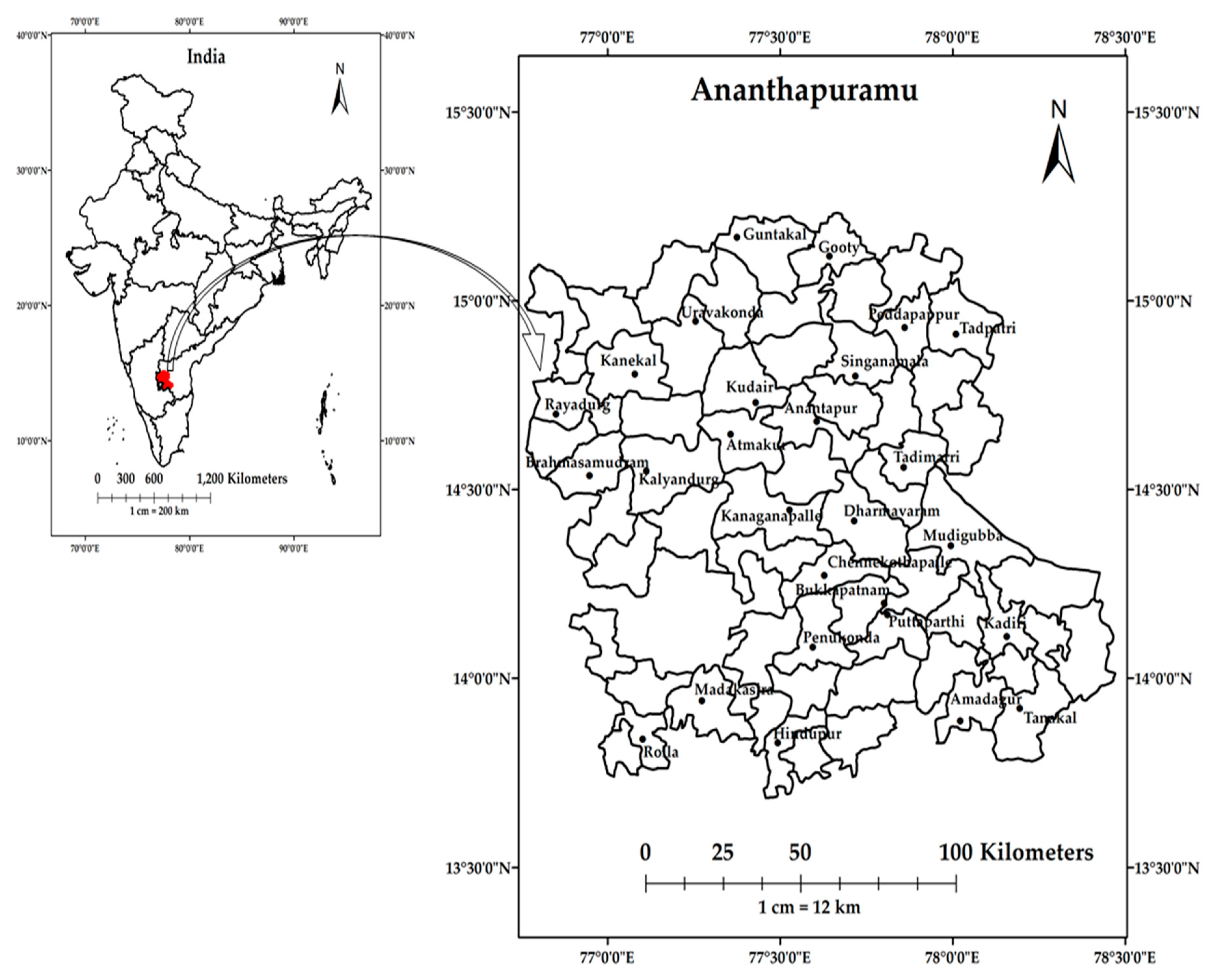
The Ananthapuramu district is in the southern part of India, in the state of Andhra Pradesh. The district lies between 13°40′ N to 15°15′ N latitude and 76°50′ E to 78°30′ E longitude. It is the largest district in the state with 63 subdistricts covering an area of 19,130 km². The total population of the district is 4,081,148 with a sex ratio of 977 females for every 1000 males. The literacy rate of the district is 64.28 percent [67]. Most of the cultivated area in the district is rainfed and only a small portion of land is under irrigated agriculture. The soils in the district are mostly red soils with 76% of the total area, and the remaining 24% are black soils. The soil texture is predominantly sandy loam with low water retention capacity. Soil moisture deficiency is commonly observed in the area during all stages of crop growth, leading to frequent crop failures [60]. The average elevation of the district is 610 m with the lowest elevation of 230 m at Tadipatri. The elevation at Anantapuramu city is 335 m. Climatologically, the rainfall is divided into four seasons, namely winter (January and February), summer (March to May), southwest monsoon (June to September), and northeast monsoon (October to December). The district receives a normal rainfall of 553 mm. The southwest monsoon rainfall is predominant in the region, with normal rainfall of 338 mm and normal rainfall for the northeast monsoon is recorded as 156 mm. Geographically, Ananthapuramu falls away from the east coast, causing it to receive less rainfall during northeast monsoons. The district also receives precarious rainfall due to less penetration of southwest monsoons caused by high Western Ghats [67]. The annual mean maximum temperature is 33.7 °C and the minimum mean temperature is 22.0 °C [56]. Potential evapotranspiration during a southwest monsoon is higher than the total rainfall, causing serious crop stress conditions during the growing season [60]. A location map of the study area with the spatial distribution of rain gauge stations is shown in Figure 1.

The daily rainfall data for 63 subdistrict rain gauge locations are collected for the period from 1981 to 2016 from the Department of Statistics and Planning, Ananthapuramu. The observations started from the year 1987 at Amadagur, Brahmasamudram, Mudigubba, Peddapappur, Puttaparthi, Rolla, and Tadimarri stations. Any station with more than 10 percent missing data is not considered for the analysis. After careful preprocessing for missing data and quality checks, a total of 27 rain gauge locations were selected for homogeneity and trend analysis. Daily rainfall data is aggregated to the number of rainy days and total rainfall at a monthly, seasonal, and annual scale. According to Indian Meteorological Department standards, a given day is considered as a rainy day if the total accumulated rainfall is more than 2.5 mm. India Meteorological Department’s high resolution, gridded rainfall data at 0.25° × 0.25° resolution [68] is used in the study to validate the rain gauge level findings. The daily gridded data is also aggregated to a monthly, seasonal, and annual scale for the purpose of analysis. Geographical location and elevation information of the rain gauge stations and the corresponding length of the data record is provided in

Table 1. Description of rain gauge locations in the study area considered for analysis.

Serial Number	Station	Latitude	Longitude	Elevation (in Meters)	Record Period
1	Amadagur	13°53′	78°01′	675	1987–2016
2	Anantapur	14°40′	77°36′	352	1981–2016
3	Atmakur	14°38′	77°21′	497	1981–2016
4	Brahmasamudram	14°32′	76°56′	511	1987–2016
5	Bukkapatnam	14°11′	77°48′	445	1981–2016
6	Chennekothapalle	14° 16′	77°37′	438	1981–2016
7	Dharmavaram	14°24′	77°43′	376	1981–2016
8	Gooty	15°07′	77°38′	384	1981–2016
9	Guntakal	14°09′	77°23′	456	1981–2016
10	Hindupur	13°49′	77°29′	626	1981–2016
11	Kadiri	14°06′	78°09′	520	1981–2016
12	Kalyandurg	14°32′	77°06′	556	1981–2016
13	Kanaganapalle	14°26′	77°31′	436	1981–2016
14	Kanekal	14°48′	77°04′	456	1981–2016
15	Kudair	14°43′	77°25′	422	1981–2016
16	Madakasira	13°56′	77°16′	664	1981–2016
17	Mudigubba	14°20′	77°57′	404	1987–2016
18	Peddapappur	14°55′	77°51′	262	1987–2016
19	Penukonda	14°04′	77°35′	566	1981–2016
20	Puttaparthi	14°10′	77°48′	459	1987–2016
21	Rayadurg	14°41′	76°51′	555	1981–2016
22	Rolla	13°50′	77°06′	715	1987–2016
23	Singanamala	14°48′	77°43′	310	1981–2016
24	Tadimarri	14°33′	77°51′	317	1987–2016
25	Tadpatri	14°54′	78°00′	238	1981–2016
26	Tanakal	13°55′	78°11′	612	1981–2016
27	Uravakonda	14°56′	77°15′	479	1981–2016

.

3. Methodology

Various statistical tests were performed to analyze the homogeneity, trends, and trend change points in the time series data, after thorough quality checks and preprocessing. The sequential stages in data analysis are:

• Homogeneity tests;
• Testing for serial correlation;
• Trend tests;
• Trend change-point tests.

3.1. Homogeneity Tests

Homogeneity testing is very crucial in climatological studies to represent the real variations in weather and climate. Inhomogeneity occurs in climate data due to several reasons including instrumentation error, changes in the adjacent areas of the instrument, and mishandling of the human. If the homogeneity is not tested prior to trend analysis, the results will indicate erroneous trends. In this study, the absolute homogeneity tests were performed on individual station records and relative homogeneity tests were performed by generating a reference series using Anclim software package and calculating the ratio of observed series to the reference series [69,70,71]. Four widely used statistical tests mentioned below were applied to the data to test for homogeneity. All of the following four tests used in this study assume the null hypothesis of data being homogeneous:

• Alexandersson’s standard normal homogeneity test [69,70];
• Buishand’s range test [72];
• Pettitt’s test [73];
• Von Neumann’s ratio test [74].

3.1.1. Alexandersson’s Standard Normal Homogeneity Test

For an annual series $X_i$ (i is the year from 1 to n) with mean “$\overline{X}$” and standard deviation “$s$”, Alexandersson (1986) [69,70] describes a statistic $T\left(k\right)$ to compare the mean of first “$k$” years of the record with that of last “$n-k$” years as

$$T\left(k\right)=k{\overline{z}}_1^2+\left(n-k\right){\overline{z}}_2^2\mathrm{for}k=1, 2, \dots , n$$

(1)

where,

$${\overline{z}}_1=\frac{1}{k}{{\displaystyle \sum }}_{i=1}^k\frac{\left(X_i-\overline{X}\right)}{s}\mathrm{and}{\overline{z}}_2=\frac{1}{\left(n-k\right)}{{\displaystyle \sum }}_{i=k+1}^n\frac{\left(X_i-\overline{X}\right)}{s}$$

(2)

If a break is located at year “K”, then $T\left(k\right)$ reaches a maximum near the year k = K. The test statistic $T_0$ is defined as

$$T_0=\underset{1\le k<n}{\max }T\left(k\right)$$

(3)

The null hypothesis is rejected when $T_0$ is above the critical value, which depends on the sample size. The critical values for various sample sizes starting from 10 to 5000 are given in Khaliq et al. [75].

3.1.2. Buishand’s Range Test

In Buishand’s range test [72], for an annual series $X_i$ (i is the year from 1 to n) with mean “$\overline{X”}$ and standard deviation “$s$”, the adjusted partial sums, are defined as

$$S_0^{\ast }=0and{S}_k^{\ast }={{\displaystyle \sum }}_{i=1}^k\left(X_i-\overline{X}\right)\mathrm{where}k=1,2,\dots ,n$$

(4)

For a homogeneous series, the value of $S_k^{\ast }$ fluctuates around zero, as no systematic deviations of the $X_i$ values with respect to their mean will appear. When a break point is present in the series, the $S_k^{\ast }$ value reaches a maximum value (negative shift) or minimum value (positive shift) near the year k = K. The $(S_k^{\ast }/s)/\sqrt{n}$ is depicted in the graphs representing the results of this test. The significance of the shift can be tested using ”rescaled adjusted range” denoted as R, which is the difference between the maximum and minimum of the $S_k^{\ast }$ values scaled by the sample standard deviation.

$$R=\left(\underset{0\le k\le n}{\max }{S}_k^{\ast }-\underset{0\le k\le n}{\min }{S}_k^{\ast }\right)/S$$

(5)

$R/\sqrt{n}$ value is compared with the critical values of Buishand (1982) [72] to test for significance.

3.1.3. Pettitt’s Test

Pettitt’s test [73] is a nonparametric rank test. The ranks $r_1,r_2,$ …$, r_n$ of the series $X_1,X_2,$ …$,X_n$ are used to calculate the test statistics as

$$Y_k=2{{\displaystyle \sum }}_{i=1}^k{r}_i-k\left(n+1\right)\mathrm{where}k=1,2,\dots ,n$$

(6)

When a break occurs at year K, the statistic is maximum or minimum at year k = K,

$$Y_{\mathrm{K}}=\underset{1\le k\le n}{\max }\left|Y_k\right|$$

(7)

The value of $Y_{\mathrm{K}}$ is compared with critical values given by Pettitt (1979) [73] to test for statistical significance.

3.1.4. Von Neumann’s Ratio Test

For an annual series $X_i$ (i is the year from 1 to n) with mean “$\overline{X}$”, The von Neumann ratio “$N$” is defined as the ratio of the mean square successive (year to year) difference to the variance, given as

$$N={{\displaystyle \sum }}_{i=1}^{n-1}{\left(X_i-X_{i+1)}\right)}^2/{{\displaystyle \sum }}_{i=1}^n{\left(X_i-\overline{X}\right)}^2$$

(8)

If there is a break in the series, the value of $N$ tends to be lower than the expected value. If there is a rapid variation in the mean, the values of $N$ may rise above two. This test does not indicate the exact location of the break year.

3.2. Testing for Serial Correlation

To detect the trend in a time series, the statistical tests assume the subsequent data in the series to be independent. The power of trend tests is highly influenced by the presence of serial correlation in the data [44,76]. A positive serial correlation leads to wrongful rejection of the null hypothesis of no trend when it is true (type I error). Similarly, a negative serial correlation leads to accepting the null hypothesis of no trend when it is false (type II error). To test for serial correlation in the data, lag−1 serial correlation coefficients are calculated [77,78,79,80,81]. In several of the trend studies, the time series is tested for serial correlation by calculating the lag−1 serial correlation coefficient ${\mathsf{\rho }}_1$ [82,83,84,85]. For any time series $X_i=x_1,x_2, \dots , x_n$, lag−1 serial correlation coefficient (${\mathsf{\rho }}_1$) is calculated as

$${\mathsf{\rho }}_1=\frac{\frac{1}{n-1}{{\displaystyle \sum }}_{i=1}^{n-1}\left(x_i-E\left(x_i\right)\right).\left(x_{i+1}-E\left(x_i\right)\right)}{\frac{1}{n}{{\displaystyle \sum }}_{i=1}^n{\left(x_i-E\left(x_i\right)\right)}^2}$$

(9)

where $E\left(x_i\right)$ is the mean of the sample and $n$ is the sample size

$$E\left(x_i\right)=\frac{1}{n}{{\displaystyle \sum }}_{i=1}^n{x}_i$$

(10)

The probability limits for ${\mathsf{\rho }}_1$ on the correlogram of an independent series is given by Anderson (1941) [81] as

$${\mathsf{\rho }}_1=\{\begin{array}{c}\frac{-1+1.645\sqrt{n-2}}{n-1} , \mathrm{for} \mathrm{the} \mathrm{one}-\mathrm{tailed} \mathrm{test}\\ \frac{-1\pm 1.96\sqrt{n-2}}{n-1} , \mathrm{for} \mathrm{the} \mathrm{two}-\mathrm{tailed} \mathrm{test}\end{array}$$

(11)

Significance of serial correlation was evaluated by comparing the ${\mathsf{\rho }}_1$ value with the critical values of Student’s t-distribution values.

3.3. Trend Tests

Trends tests are applied to time series data to identify significant positive or negative trends. All the trend tests in this section assume the null hypothesis of no trend and the alternative hypothesis of monotonic increasing or decreasing trend existence. When the time series are serially independent, the Mann–Kendall test [36,37] and Spearman’s Rho test [38,39] were applied to test for trends. These two tests are very robust in detecting the trends and are widely used in literature. The magnitude of the trend was estimated using Sen’s slope method [40,41]. From the extensive literature survey, it is evident that there is no universal solution to account for serial correlation present in the time series. It is always suggested to apply various statistical tests to analyze the trends in serially correlated data. In this study, when the time series exhibit a significant serial correlation, the following modified versions of the Mann–Kendall test were used:

• Pre-whitening [35,43];
• Trend-ree pre-whitening [44];
• Bias-correction applied to pre-whitening [45];
• Variance correction approach suggested by Hamed and Rao, 1998 (MMKH) [46];
• Variance correction approach suggested by Yue and Wang, 2004 (MMKY) [47].

3.3.1. Mann–Kendall Test

The Mann–Kendall test [36,37] is perhaps the most widely used nonparametric test for detecting trends in hydro-meteorological and environmental data. The Mann–Kendall test is a nonparametric test for monotonic trend detection. It does not assume the data to be normally distributed and is flexible to outliers in the data. The test assumes a null hypothesis, H₀, of no trend and alternate hypothesis, H_A, of increasing or decreasing monotonic trend.

For a time series $X_i=x_1,x_2, \dots , x_n$, the Mann–Kendall test statistic $S$ is calculated as

$$S={{\displaystyle \sum }}_{i=1}^{n-1}{{\displaystyle \sum }}_{j=i+1}^{n}sign\left(x_j-x_i\right)$$

(12)

where $n$ is the number of data points, $x_i$ and $x_j$ are the data values in timeseries $i$ and $j$ ($j>i)$, respectively, and $sign\left(x_j-x_i\right)$ is the sign function as

$$Sign\left(x_i-x_j\right)=\{ \begin{array}{cc}-1& if \left(x_j-x_i\right)<0\\ 0& if \left(x_j-x_i\right)=0 \\ 1& if \left(x_j-x_i\right)>0\end{array}$$

(13)

Statistics $S$ is normally distributed with parameters $E\left(S\right)$ and variance $V\left(S\right)$ as given below:

$$E\left(S\right)=0$$

(14)

$$V\left(S\right)=\frac{n\left(n-1\right)\left(2n+5\right)-{{\displaystyle \sum }}_{k=1}^m{t}_k\left(k\right)\left(k-1\right)\left(2k+5\right)}{18}$$

(15)

where $n$ is the number of data points, $m$ is the number of tied groups, and $t_k$ denotes the number of ties of extent $k$. Standardized test statistic $Z$ is calculated using the formula below.

$$Z=\{\begin{array}{cc}\frac{S-1}{\sqrt{var\left(S\right)}}& if S>0\\ 0& if S=0\\ \frac{S+1}{\sqrt{var\left(S\right)}}& if S<0\end{array}$$

(16)

To test for a monotonic trend at an α significance level, the alternate hypothesis of trend is accepted if the absolute value of standardized test statistic Z is greater than the Z_{1 − α/2} value obtained from the standard normal cumulative distribution tables. A positive sign of the test statistic indicates an increasing trend and a negative sign indicates a decreasing trend.

3.3.2. Spearman’s Rank Correlation Coefficient Test

The Spearman’s Rho test [38,39] is another widely used nonparametric test. The power of this test is comparable with the Mann–Kendall test [42]. For a given time series $X_i=x_1,x_2, \dots , x_n$, the spearman rank correlation coefficient ${\mathrm{r}}_{\mathrm{SRC}}$ is given as

$${\mathrm{r}}_{\mathrm{SRC}}=1-\left\{\frac{6{{\displaystyle \sum }}_{i=1}^n{\left[d_i\right]}^2}{n\left(n^2-1\right)}\right\}$$

(17)

where $d_i=\left(R{X}_i-R{Y}_i\right)$. $R{X}_i$ is the rank of the variable $X_i$, $R{Y}_i$ is the chronological order of observations and $i=1, 2, \dots , n$ in series of size $n$. The test statistic ${\mathrm{t}}_{\mathrm{SRC}}$ is given by Equation (18).

$${\mathrm{t}}_{\mathrm{SRC}}={\mathrm{r}}_{\mathrm{SRC}}\sqrt{\frac{\left(n-2\right)}{1-{\mathrm{r}}_{\mathrm{SRC}}^2}}$$

(18)

Test statistic ${\mathrm{t}}_{\mathrm{SRC}}$ follows a t−distribution with the degree of freedom ν and significance level α. The null hypothesis of no trend is rejected when $\left|{\mathrm{t}}_{\mathrm{SRC}}\right|>{\mathrm{t}}_{\mathsf{\nu },1-\left(\mathsf{\alpha }/2\right)}$.

3.3.3. Sen’s Slope Estimator

The Sen’s slope method is a robust nonparametric method of estimating the magnitude of trend slope [40,41]. For a given time series $X_i=x_1,x_2, \dots , x_n$, with N pairs of data, the slope is calculated as given in Equation (19)

$${\beta }_i=\frac{x_j-x_k}{j-k}, \forall k\le j\mathrm{and}i=1, 2, \dots , N$$

(19)

Median of N values of ${\beta }_i$ gives the Sen’s estimator of slope $\beta$.

$$\beta =\{\begin{array}{cc}\frac{{\beta }_{N+1}}{2},\hfill & \mathrm{if} N \mathrm{is} \mathrm{odd}\\ \frac{\left(\frac{{\beta }_{\mathrm{N}}}{2}+\frac{{\beta }_{N+2}}{2}\right)}{2},\hfill & \mathrm{if} N \mathrm{is} \mathrm{even}\end{array}$$

(20)

3.3.4. Pre-Whitening

For a given time series $X_i=x_1,x_2, \dots x_n$, with lag−1 serial correlation coefficient ${\mathsf{\rho }}_1$ as mentioned in Equation (9), pre-whitened series $X_t^{\prime }$ is given by von Storch (1995) [35,43] as

$$X_t^{\prime }=X_t-{\mathsf{\rho }}_1{X}_{t-1}$$

(21)

3.3.5. Trend-Free Pre-Whitening

In trend-free pre-whitening [44] of a given timeseries $X_t=x_1,x_2,\dots ,x_n$, the first step is to calculate the Sen’s slope using Equations (19) and (20). The monotonic trend $\beta$ is removed from $X_i$ to form a trend-free series $y_t$

$$y_t=x_t-\beta t$$

(22)

where $x_t$ is the series value at time $t$, $y_t$ is the de−trended series, and $\beta$ is the trend slope.

In the next stage, lag−1 serial correlation coefficient ${\mathsf{\rho }}_1$ of the detrended series $y_t$ is calculated as mentioned in Equation (9). If ${\mathsf{\rho }}_1$ is not significant, the trend detection is performed on the detrended series. In case of significant serial correlation at lag−1, the detrended series is pre-whitened and the residual series $y_t^{\prime }$ is calculated as

$$y_t^{\prime }=y_t-{\mathsf{\rho }}_1{y}_{t-1}$$

(23)

In the final stage, the monotonic trend component is added back to residual series $y_t^{\prime }$ to generate the trend-free pre-whitening series $X_t^{\ast }$

$$X_t^{\ast }=y_t^{\prime }+\beta t$$

(24)

3.3.6. Bias-Corrected Pre-whitening

A time series $X_t=x_1, x_2,\dots , x_{n,}$ assumed to follow a first ordered serial correlation process including a linear trend can be modeled as

$$X_t=\mathsf{\rho }{X}_{t-1}+\alpha +\beta t+{\epsilon }_t$$

(25)

where $X_t$ and $X_{t-1}$ are observations at times t and t − 1, respectively; $\mathsf{\rho }$ is the serial correlation coefficient; $\alpha$ is constant intercept term; $\beta$ is trend slope with respect to time; and ${\epsilon }_t$ is an uncorrelated noise term. The estimated values of $\mathsf{\rho },\alpha , \mathrm{and} \beta$ are given by the matrix calculation below

$${\left[\begin{array}{ccc}\mathsf{\rho }& \alpha & \beta \end{array}\right]}^T={\left(Z^{T}Z\right)}^{-1}{Z}^{T}y$$

(26)

where Z is the matrix of size $\left(n-1\right)·3$ whose second column contains $\left(n-1\right)$ values equal to 1, and the third column contains the numbers 2 to $n$ and $y$ is a vector of size $\left(n-1\right)·1$ containing the observations $x_2$ to $x_n$. The bias-corrected serial correlation coefficient ${\mathsf{\rho }}^{\ast }$ [45,86] is calculated using the formula mentioned in Equation (27). This value is used in bias-corrected pre-whitening and trend detection studies.

$${\mathsf{\rho }}^{\ast }=\frac{(n\widehat{\mathsf{\rho }}+2)}{n-4}$$

(27)

3.3.7. Variance Correction Approaches

In a time series $X_t=x_1,x_2,\dots , x_{n,}$ with $n$ number of observations, effective information is contained in $n^{\ast }$ number of observations. Effective sample size $n^{\ast }$ is always less than the original sample size $n$. In the presence of positive or negative serial correlation, the variance of the Mann–Kendall test statistic $S$ increases or decreases, respectively. This effect can be reduced by calculating the modified variance $V^{\ast }\left(S\right)$.

$$V^{\ast }\left(S\right)=V\left(S\right)\ast CF$$

(28)

Correction factors (CF) proposed by Hamed and Rao (1998) [46] and Yue and Wand (2004) [47] termed as CF₁ and CF₂, respectively are

$$C{F}_1=1+\frac{2}{n\left(n-1\right)\left(n-2\right)}{\displaystyle \sum }_{k=1}^{n-1}\left(n-k\right)\left(n-k-1\right)\left(n-k-2\right)r_k^R$$

(29)

$$C{F}_2=1+2{{\displaystyle \sum }}_{k=1}^{n-1}\left(1-\frac{k}{n}\right)r_k$$

(30)

where $r_k and r_k^R$ are the $lag-k$ serial correlation coefficients of data and ranks of data respectively and $n$ is the total length of the series. In the case of $C{F}_1$ only significant correlation coefficients are used. For calculating $C{F}_2$, $lag-1$ serial correlation coefficient is used. The Mann–Kendall trend test is calculated by using corrected variance $V^{\ast }\left(S\right).$

3.4. Trend Change-Point Tests

In hydroclimatic trend analysis, identifying the trends and time of trend change both play a significant role. Any trend detection study is incomplete without reporting the time of trend change. Unfortunately, none of the previous studies in the region have reported the starting time of significant rainfall trends. In this study, the distribution-free CUSUM test [62] and sequential Mann–Kendall test [63,64] were employed in the trend change-point analysis. Both these tests are nonparametric tests and are very useful for identifying sequential step changes in the time series. The CUSUM test [62] is based on cumulative sum charts and the sequential Mann–Kendall test [63,64] considers each sample point sequentially considered in both a progressive and retrograde manner.

3.4.1. Distribution-Free CUSUM Test

The distribution-free CUSUM test [62] checks that differences in the mean values in two parts of a series are different for an unknown time. The median value of the series is compared with successive values in order to detect the change after a number of observations. The test statistic, $V_k$, is the maximum value of the cumulative sum (CUSUM) of the $k$ signs of differences from the median (which is a series of −1 or +1) starting from the beginning of the series. For a time series $X_t=x_1,x_2, \dots , x_n,$ the test statistic $V_k$ is given as

$$V_k={\displaystyle \sum }_{i=1}^{k}sign\left(x_i-x_{median}\right)\mathrm{where},k=1, 2, \dots , n$$

(31)

where $k=1,2,\dots ,n$ and $sign\left(x_i-x_{median}\right)$ is given as

$$Sign\left(x_i-x_{median}\right)=\{\begin{array}{cc}-1& if \left(x_i-x_{median}\right)<0\\ 0& if \left(x_i-x_{median}\right)=0 \\ 1& if \left(x_i-x_{median}\right)>0\end{array}$$

(32)

The distribution of $V_k$ follows the Kolmogorov–Smirnov two-sample statistic $KS=\left(\frac{2}{n}\right)\max \left|V_k\right|$, with a critical value of $\max \left|V_k\right|$ given at various significance levels as in Equation (33)

$$\begin{array}{c}1.22\sqrt{n} at \alpha =0.10\\ 1.36\sqrt{n} at \alpha =0.05\\ 1.63\sqrt{n} at \alpha =0.01\end{array}$$

(33)

3.4.2. Sequential Mann–Kendall Test

For a series $X_t=x_1, x_2,\dots , x_n,$ the sequential Mann–Kendall test is a rank-based test to identify the change point in the time series. From Taubenheim (1989) [63] and Sneyers (1990) [64], the first step is to arrange the series as ranked order and calculating the test statistic $t_j$

$$t_j={\displaystyle \sum }_i^j{n}_j$$

(34)

where $n_j$ is the number of times $x_{j >}{x}_i$ under the condition $j>i$ with $j=1, 2, \dots , n$ and $i=1, 2,\dots , j-1$.

The distribution of the test statistic is asymptotically normal with mean $E(t_j)=\frac{j\left(j-1\right)}{4}$ and variance $VAR(t_j)=\frac{j\left(j-1\right)\left(2j+5\right)}{72}$. A reduced variable called prograde series $u\left(t\right)$ is calculated for each of the test statistic variables, $t_j$, as

$$u\left(t\right)=\frac{t_j-E\left(t_j\right) }{\sqrt{VAR\left(t_j\right)}}$$

(35)

In a similar way, retrograde series $u^{\prime }\left(t\right)$ is calculated from the end of the series. In the absence of a trend, the series intersects at several locations. In the presence of a significant trend, the point of intersection of the prograde series and the retrograde series indicates the trend change point.

3.5. Software Packages, “modifiedmk” and “trendchange”

Two open-source library packages namely “modifiedmk” and “trendchange” were developed in R-language [87]. The package “modifiedmk” was used to perform the nonparametric Mann–Kendall test, Spearman’s rank correlation coefficient test and all modified versions of the Mann–Kendall test mentioned in this study. Another package “trendchange” was used for change-point analysis. These packages are now freely available via CRAN repository and Github version control platform [65,66].

4. Results and Discussion

Each station contains 17 series (12 monthly, one annual and four seasonal series), and a total of 459 time series generated from 27 rain gauge locations (27 × 17) were subjected to statistical tests and the analysis is provided in this section. Absolute homogeneity and relative homogeneity tests were reported at a confidence interval of 95%. Results of the trend tests are reported at 90%, 95%, and 99% confidence intervals. Trend change points are reported when there is any significant positive or negative trend observed in the time series.

4.1. Homogeneity of Rainfall Data

The results of the absolute homogeneity tests and relative homogeneity tests are grouped into three classes as follows:

• Useful, if none or only one of the above four tests reject the null hypothesis;
• Doubtful, if two of the four tests reject the null hypothesis;
• Suspect, if three or all the tests reject the null hypothesis.

A similar type of classification is observed in Schönwiese and Rapp (1997) [88] and Wijngaard et al. [89]. Out of 459 series, all the records of Bukkapatnam, Dharmavaram, Hindupur, Kadiri, Madakasira, Puttaparthi, Rolla, and Tanakal stations found as ”useful” in both absolute and relative homogeneity tests, and hence are not mentioned in the summary of homogeneity analysis, as depicted in

Table 2. Summary of homogeneity results.

Station Name	Absolute Homogeneity		Relative Homogeneity
	Doubtful	Suspect	Doubtful	Suspect
Amadagur	-	-	January	-
Anantapur	-	-	September	-
Atmakur	May October	Annual Summer Southwest monsoon	-	January September
Brahmasamudram	-	-	Annual Northeast monsoon	January
Chennekothapalle	January September October	-	-	Annual
Gooty	April Summer	-	April	-
Guntakal	January	April May Summer	-	-
Kalyandurg	-	Summer	-	-
Kanaganapalle	-	Summer	Northeast monsoon	-
Kanekal	December	Summer	-	-
Kudair	March	August Annual Summer	September	January
Mudigubba	-	-	-	January
Peddapappur	February March	-	Annual	February
Penukonda	April October Summer	-	-	-
Rayadurg	December	Summer	-	September
Singanamala	May October	-	October Northeast monsoon	Annual
Tadimarri	-	January	Annual	January
Tadpatri	October	-	-	Annual
Uravakonda	Summer	-	Winter	-

.

The absolute homogeneity test results indicated 20 series as “doubtful” and 14 series as “suspect”, and all the remaining as “useful”. Relative homogeneity test results indicated 12 series to be “doubtful” and 11 series to be “suspect” and the remaining series to be “useful”. Any series classified as a suspect is considered inhomogeneous and excluded from trend analysis.

4.2. Serial Correlation Analysis

The serial correlation test is highly influenced by the confidence interval used in the statistical tests. The results of this study indicated 26 series out of 459 series found to be serially correlated at a 90% confidence interval. The critical values for the serial correlation test are calculated as per Equation (11). For any series with 36 observations, the critical value is ± 0.274 and for the series with 30 observations, the critical value is ± 0.3. At a confidence interval of 95%, the number of series influenced by serial correlation reduced drastically by half to 13. Analysis at the 99% confidence interval indicated only two series were affected by serial correlation.

4.3. Rainfall Trend Analysis

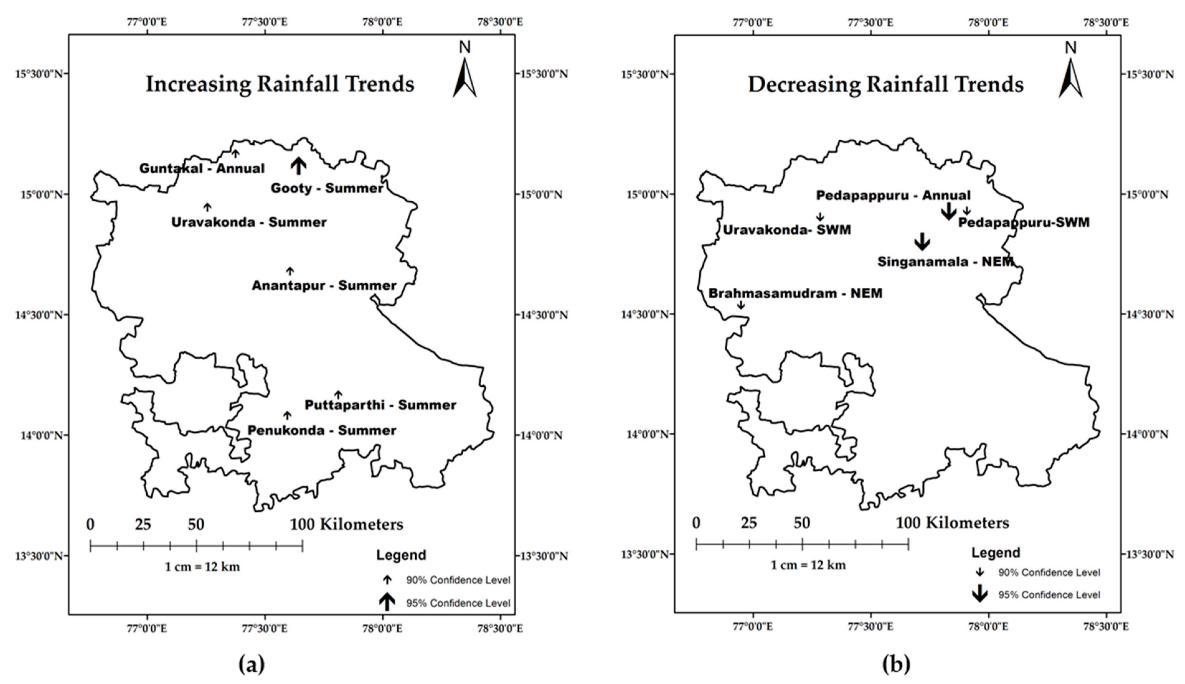
Trend analysis is performed on a monthly, annual, and seasonal rainfall series, and the results of serially independent annual and seasonal rainfall alone are shown in

Table 3. Results of the Mann–Kendall (MK) test, Sen’s Slope test (SS), and Spearman’s rank correlation coefficient (SRC) test without considering the effect of serial correlation.

Station Name	Annual			Winter			Summer			Southwest Monsoon			Northeast Monsoon
	MK	SS	SRC	MK	SS	SRC	MK	SS	SRC	MK	SS	SRC	MK	SS	SRC
Amadaguru	−1.070	−3.674	−1.120	0.946	0.000	1.462	0.946	1.417	1.010	−0.856	−2.552	−0.837	−0.357	−0.933	−0.213
Anantapur	0.150	0.349	0.307	1.158	0.000	1.473	1.703 *	1.825	1.750 *	−0.477	−1.254	−0.338	−0.708	−0.767	−0.745
Atmakur	IH	IH	IH	1.090	0.000	1.724 *	IH	IH	IH	IH	IH	IH	0.913	1.008	0.953
Brahmasamudram	−1.534	−5.906	−1.622	0.535	0.000	0.801	0.999	1.129	1.244	−1.285	−4.447	−1.171	−1.820 *	−3.165	−1.705 *
Bukkapatnam	0.150	0.583	0.173	0.150	0.000	0.295	1.267	0.974	1.569	−0.014	−0.073	0.116	−0.449	−0.787	−0.499
Chennekottapalle	IH	IH	IH	1.539	0.000	2.131 #	0.844	0.495	0.746	−0.341	−0.729	−0.278	−0.640	−1.005	−0.797
Dharmavaram	0.000	−0.102	−0.077	0.504	0.000	0.554	1.171	1.030	1.213	−0.313	−0.827	−0.171	SC	SC	SC
Gooty	−0.218	−0.711	−0.179	0.163	0.000	0.318	2.438 #	1.811	2.673 ⸸	−1.022	−2.051	−0.843	−0.014	−0.007	−0.094
Guntakal	1.839 *	4.805	1.822 *	1.131	0.000	1.642	IH	IH	IH	0.613	1.123	0.666	0.804	0.819	0.817
Hindupur	−0.204	−0.675	−0.272	SC	SC	SC	1.566	1.490	1.616	−0.817	−2.299	−0.773	−0.177	−0.176	−0.028
Kadiri	−0.259	−0.776	−0.202	−0.014	0.000	−0.041	1.444	1.243	1.729 *	−0.286	−1.118	−0.536	0.000	0.004	0.253
Kalyanadurg	1.076	3.322	1.215	0.395	0.000	0.729	IH & SC	IH & SC	IH & SC	0.477	0.855	0.633	0.000	0.060	0.402
Kanaganapalle	0.041	0.124	0.236	1.022	0.000	1.394	IH	IH	IH	−0.232	−0.578	−0.202	−0.885	−0.894	−0.547
Kanekal	SC	SC	SC	0.095	0.000	0.231	IH	IH	IH	0.232	0.758	0.283	−0.041	−0.106	−0.317
Kudair	IH	IH	IH	1.553	0.000	2.525 #	IH	IH	IH	0.477	0.942	0.573	0.558	0.461	0.528
Madakasira	−0.150	−0.296	−0.187	0.790	0.000	1.243	1.566	1.726	1.636	−0.422	−0.950	−0.581	0.259	0.467	0.746
Mudigubba	−0.963	−4.740	−0.949	0.553	0.000	0.783	0.321	0.250	0.301	−1.213	−4.088	−0.974	SC	SC	SC
Pedapappuru	−2.034 #	−7.648	−2.053 #	0.517	0.000	0.633	0.517	0.447	0.656	−1.820 *	−4.750	−1.827 *	−1.606	−3.189	−1.449
Penukonda	SC	SC	SC	1.131	0.000	1.514	1.866 *	1.901	2.080 #	SC	SC	SC	0.831	1.166	1.033
Puttaparthi	SC	SC	SC	0.571	0.000	0.887	1.659 *	1.763	1.716 *	−0.285	−1.413	−0.269	−0.731	−1.308	−0.760
Rayadurg	0.667	2.201	0.663	0.313	0.000	0.512	IH	IH	IH	−0.082	−0.207	−0.078	SC	SC	SC
Rolla	−1.606	−7.135	−1.688 *	−0.054	0.000	−0.061	0.178	0.240	0.335	−0.821	−3.933	−0.879	−1.392	−3.300	−1.444
Singanamala	IH	IH	IH	1.158	0.000	1.465	0.000	−0.005	−0.041	−1.103	−2.429	−1.032	−2.411 #	−2.716	−2.221 #
Tadimarri	−0.285	−1.175	−0.264	1.463	0.000	2.172 #	0.821	0.692	1.032	−0.071	−0.117	0.001	SC	SC	SC
Tadipatri	IH	IH	IH	0.640	0.000	0.852	0.123	0.074	0.139	−0.749	−2.002	−0.678	−0.736	−1.179	−0.826
Tanakal	−0.245	−1.052	−0.211	0.913	0.000	1.280	0.640	0.504	0.601	−0.504	−1.506	−0.443	−0.667	−0.799	−0.615
Uravakonda	SC	SC	SC	0.613	0.000	1.011	1.812 *	1.241	1.961 #	−1.703 *	−3.706	−1.883 *	−1.076	−1.633	−0.934

*, significant at a 90% confidence interval; #, significant at a 95% confidence interval; and ⸸, significant at a 99% confidence interval. IH, inhomogeneous; SC, serially correlated.

. The spatial location of the stations with increasing and decreasing rainfall trends are as shown in Figure 2.

Trend analysis indicated both increasing and decreasing trends in annual rainfall. Increasing annual rainfall trend is observed at the Guntakal station at a 90% confidence interval (4.8 mm/year), whereas Pedapappuru annual rainfall indicated a decreasing trend at a 95% confidence interval (−7.6 mm/year). The Spearman’s rank correlation coefficient test result at the Rolla station indicated a decreasing annual rainfall trend at a confidence interval of 90% (−7.1 mm/year), while the Mann–Kendall test does not indicate any significant trend. The IMD gridded rainfall data analysis at river basin scale by Bisht et al. [8] and climate projections used in Jaspers et al. [90] showed an increasing annual rainfall trend. It is to be noted that, although the interpolated and projected climate data showed an increasing trend, the trend analysis using station level data, as in Rao et al. [8], indicated a similar increasing annual rainfall trend at the Guntakal station and decreasing annual rainfall trend at the Pedapappuru station, as in this study.

In the study area, very sparse rainfall is observed during the winter season. The Mann–Kendall test results do not indicate any significant trend in winter rainfall. The Spearman’s rank correlation coefficient test result the Atmakur station indicated an increasing winter rainfall trend at a confidence interval of 90% and Chennekottapalle, Kudair, and Tadimmari stations showed an increasing trend at a confidence interval of 95%. The magnitude of the winter rainfall trends is too small and closer to zero.

The Mann–Kendall test and Spearman’s rank correlation coefficient test indicated increasing summer rainfall at the Anantapur (1.8 mm/year) and Puttaparthi (1.7 mm/year) stations at a confidence interval of 90%. Increasing summer rainfall at the Penukonda (1.9 mm/year) and Uravakonda (1.2 mm/year) stations at a 90% confidence interval were reported by the Mann–Kendall test. Whereas, the Spearman’s rank correlation coefficient test indicated increasing trends at a confidence interval of 95% for the same stations. The SRC test results for the Gooty (1.8 mm/year) station reported increasing summer rainfall at a confidence interval of 95%, whereas the Mann–Kendall test indicated a significant increasing trend at a confidence interval of 99%. Summer rainfall series at the Kadiri station indicated an increasing trend at a 90% confidence interval (1.2 mm/year) with the Spearman’s rank correlation coefficient test, whereas the Mann–Kendall test did not indicate any significant trend. The IMD gridded rainfall data [68] and the results of Bisht et al. [8] at the river basin level also indicated increasing summer rainfall in the region.

Both the MK test and SRC test indicated decreasing southwest monsoon rainfall trend at the Pedapappuru (−4.7 mm/year) and Uravakonda (−3.7 mm/year) stations at a confidence interval of 90%. The northeast monsoon rainfall trend was decreasing at the Brahmasamudram (−3.1 mm/year) and Singanamala (−2.7 mm/year) stations at a confidence interval of 90% and 95%, respectively. The findings of the monsoon rainfall trend analysis are similar to the results of Bisht et al. [8] and Malla Reddy et al. [91]. The decrease southwest monsoon rainfall can be attributed to the geographical positioning of the district in the rain shadow region of Western Ghats. As the district is away from the coastal area, the district receives very little rainfall during the northeast monsoon season [92].

Previous studies in this region by Malla Reddy et al. [91] reported a decreasing rainfall trend during the crop growing season and an increasing rainfall outside the cropping season. It has also been reported that September rainfall, which is very crucial for Kharif cropping is declining. Early onset of summer and an increase in the temperature are causing severe soil moisture deficiency and crop failures in this region.

If a series is influenced by serial correlation, five modified versions of the Mann–Kendall test are used to examine the trends. The results of the modified Mann–Kendall tests applied to the serially correlated series at a confidence interval of 90% are shown in

Table 4. Results of modified versions of the Mann–Kendall test applied to serially correlated data.

Station Name	Time Series	PW	TFPW	BCPW	MMKH	MMKY
Amadaguru	August	−0.47	−0.17	−0.51	−1.17	−2.45 #
Brahmasamudram	June	0.54	0.51	0.43	−0.10	−0.30
Chennekothapalle	May	0.06	0.00	0.09	0.31	0.86
Dharmavaram	May	0.65	0.48	0.68	0.79	1.85 *
Dharmavaram	Northeast monsoon	−0.48	−0.37	−0.51	−0.54	−1.15
Gooty	October	0.48	0.28	0.51	0.71	0.69
Hindupur	February	−0.06	−0.06	−0.06	0.51	0.88
Hindupur	May	1.96 #	1.51	2.07 #	1.42	3.19 ⸸
Hindupur	June	0.17	0.31	0.06	0.65	1.16
Hindupur	Winter	0.30	0.30	0.30	1.40	1.79 *
Kalyanadurg	Summer	IH	IH	IH	IH	IH
Kanekal	Annual	0.28	0.28	0.48	−0.01	−0.02
Mudigubba	May	0.28	0.13	0.28	0.68	1.68 *
Mudigubba	North−east monsoon	−0.51	−0.51	−0.58	−0.10	−0.11
Pedapappuru	November	−0.09	−0.09	−0.09	−0.21	−0.50
Penukonda	Annual	0.71	1.14	0.60	0.84	1.87 *
Penukonda	Southwest monsoon	0.00	−0.17	−0.03	−0.40	−0.73
Puttaparthi	Annual	−0.54	−0.43	−0.51	−0.78	−1.32
Puttaparthi	Northeast monsoon	−1.18	−0.96	−1.14	−0.73	−2.25 #
Singanamala	May	−0.13	−0.23	−0.18	−0.64	−0.92
Tadimarri	October	−1.74 *	−1.44	−1.86 *	−1.64	−2.45 #
Tadimarri	Northeast monsoon	−0.96	−0.81	−0.99	−0.96	−2.21 #
Tadipatri	November	−0.77	−0.77	−0.82	−0.38	−0.95
Uravakonda	May	1.73 *	1.45	1.85 *	1.66 *	1.33
Uravakonda	October	−0.09	−0.03	−0.09	−0.42	−0.88
Uravakonda	Annual	−0.03	−0.57	0.00	−0.90	−2.30 #

*, significant at a 90% confidence interval; #, significant at a 95% confidence interval; and ⸸, significant at a 99% confidence interval; IH, inhomogeneous; PW, pre-whitening; TFPW, trend free pre-whitening; BCPW, bias-corrected pre-whitening; MMKH, variance correction approach suggested by Hamed and Rao; MMKY, variance correction approach suggested by Yue and Wang.

. A series is said to have a significant trend only if at least three of the five tests suggest a significant trend. The results of modified versions of the Mann–Kendall test indicated an increasing trend in May rainfall at the Hindupur and Uravakonda stations and a decreasing rainfall trend in October rainfall at the Tadimarri station. The variance correction approach suggested by Yue and Wang, 2004 [47] indicated a significant trend in most of the cases as compared with other tests.

4.4. Total Rainfall Trend versus Trend in Number of Rainy Days

In this study, we tried to examine the trend in the number of rainy days when any significant annual and seasonal trend was observed in the total rainfall. The purpose of this analysis is to examine if the trends in the number of rainy days are decreasing or increasing with the increase or decrease in the trends in the total amount of rainfall. It was observed that for winter series at the Atmakur, Kudair, Tadimarri stations; summer series at the Gooty, Kadiri sstations; and annual series at the Guntakl station, significant increasing trends were observed in both the number of rainy days and total rainfall. At the Brahmasamudram station, both trends in the number of rainy days and total rainfall were observed to be decreasing. It was observed that the number of rain days is increasing or decreasing when total rainfall is increasing or decreasing respectively.

4.5. Trend Change-Point Analysis

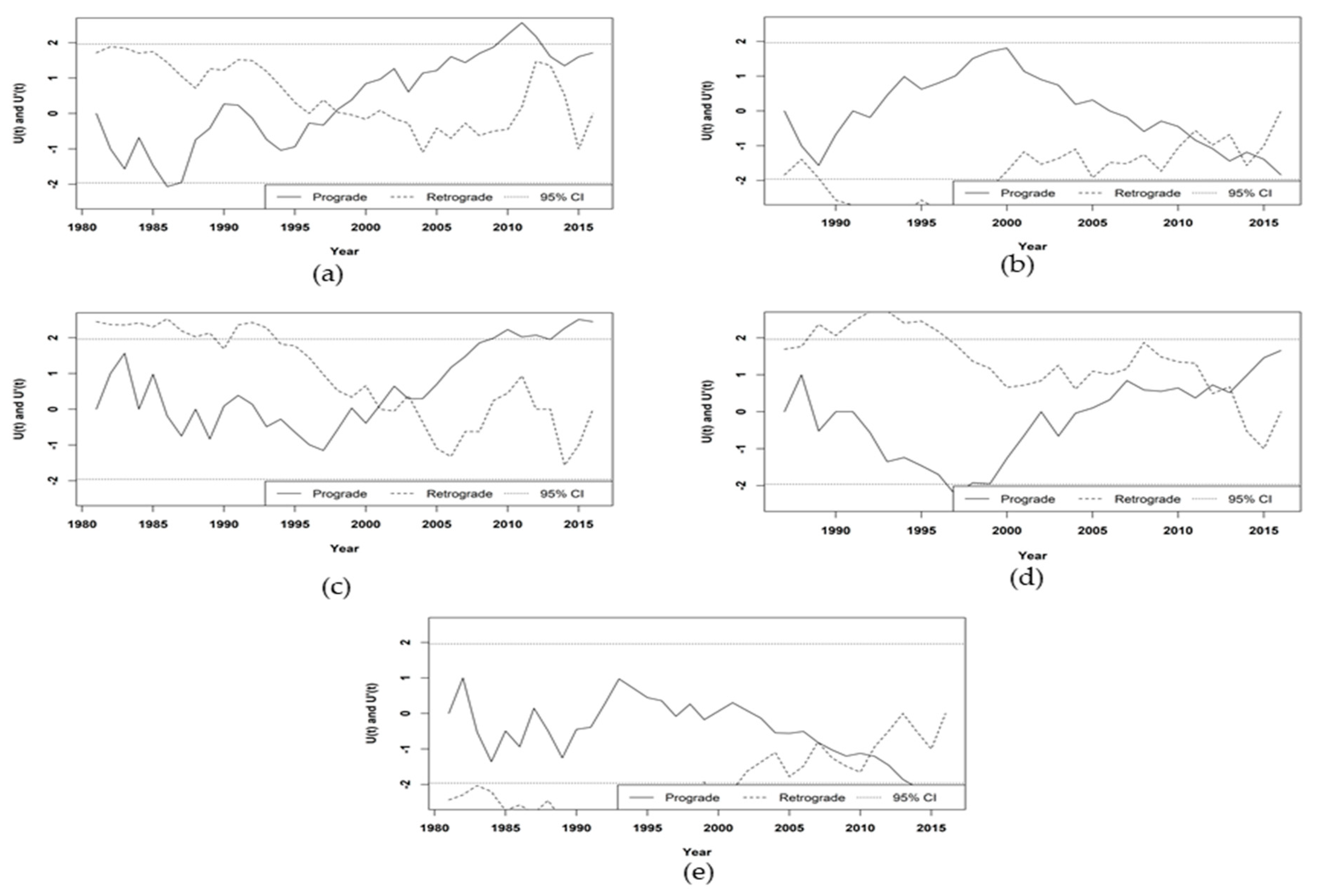
The purpose of change-point analysis is to identify the probable time where a significant change occurred in the series. Trend change-point analysis is carried out for all the series exhibiting significant trend and the results of the distribution-free CUSUM test and sequential Mann–Kendall test are shown in

Table 5. Trend change point summary.

Stations	Series	CUSUM	SQMK
Anantapur	Summer	1995 #	1998
Atmakur	Winter	2015	-
Brahmasamudram	Northeast monsoon	2003 *	2011
Chennekottapalle	Winter	2012	-
Gooty	Summer	1997 #	2001
Guntakal	Annual	1995	1995
Kadiri	Summer	1999	1995
Kudair	Winter	2012	-
Pedapappuru	Annual	2001	2011
Pedapappuru	Southwest monsoon	2001	2001
Penukonda	Summer	1999	2003
Puttaparthi	Summer	1999 *	2012
Rolla	Annual	1991	1993
Singanamala	Northeast monsoon	2002 *	2011
Tadimarri	Winter	2012	-
Uravakonda	Summer	2001	2001
Uravakonda	Southwest monsoon	2001	2012

*, significant change point at a 90% confidence interval and #, significant change point at a 95% confidence; CUSUM, distribution free CUSUM test; SQMK, sequential Mann-Kendall test.

. The CUSUM test indicated significant change points in summer series at the Anantapur, Gooty, and Puttaparthi stations, and northeast monsoon series at the Brahmasamudram and Singanamala stations.

The plots mentioned in Figure 3 are the sequential Mann–Kendall plots for significant trend change points observed with distribution-free CUSUM tests.

Sequential Mann–Kendall plots shown in Figure 3, are based on interactions between prograde and retrograde series. When a significant intersection is observed in the plot, it indicates the probable change year of the trend change. The series intersects at several locations in the absence of a significant trend. The SQMK plot of summer series at the Anantapur station (Figure 3a) indicated an increasing trend starting from 1998 and became significant from the year 2008. Around the year 2013, the positive trend started becoming insignificant. Figure 3b shows a decreasing northeast monsoon rainfall trend from 2011 and it is not found to be significant. An increasing summer rainfall trend is observed at the Gooty station (Figure 3c) starting from 2001 and a significant increase is noticed from 2008. The SQMK plot for the summer series at the Puttaparthi station is shown in Figure 3d indicated an increasing trend from the year 2012, but no significant change year is observed. Figure 3e shows a decreasing northeast monsoon rainfall trend at the Singanamala station recently, starting from 2011 and a significant decreasing year is observed around 2014.

5. Conclusions

Daily rainfall data is collected for the district of Ananthapuramu, Andhra Pradesh, India for a period of 36 years starting from 1981 and is aggregated to monthly, annual, and seasonal totals and a number of rainy days. Both absolute and relative homogeneity tests were performed on the data and inhomogeneous series were excluded from trend and change-point analysis. To implement the trend tests and change-point tests mentioned in this study, two open-source libraries were developed in R-language and are made available via CRAN repository.

The trend analysis showed increasing summer rainfall in the study area at all the stations, except for Singanamala. Six stations out of 27 stations indicated a significant increase in summer rainfall. The southwest monsoon and northeast monsoon rainfall trends are decreasing in most of the stations. Nineteen out of 27 stations indicated decreasing southwest monsoon rainfall trend and a significant decrease is observed at the Pedapappuru and Uravakonda stations. The northeast monsoon rainfall trend is decreasing at 20 stations and a significant decrease is observed at the Brahmasamudram and Singanamala stations. An increase in the summer rainfall trends and decreasing monsoon rainfall trends will impact the agriculture sector in the region.

The serial correlation was analyzed at various confidence intervals and an ensemble of modified trend tests was applied to the serially correlated data. This study is perhaps one of the few studies which considered using multiple modified versions of trend tests when the series are serially correlated. Identifying the trend change point is as crucial as studying the trends in hydro−meteorological data. The present study used two nonparametric tests to report the trend change points. Significant change points are observed in the summer season at the Anantapur, Gooty, and Puutaparthy stations and northeast monsoon season at the Brahmasamudram and Singanamala stations.

For an arid district such as Ananthapuramu, where rainfed agriculture is widely practiced, a decreasing trend in monsoon rainfall is an alarming indication. By assessing the rainfall variability, this study offers insights into distinguishing vulnerable zones within the study area so that better water management decisions, storage and irrigation infrastructure, cropping choices, and water security policies for sustainable land and water resources management can be implemented.

References

- IPCC. Climate Change 2007: Impacts, Adaptation and Vulnerability: Contribution of Working Group II to the Fourth Assessment Report of the Intergovernmental Panel; Cambridge University Press: Cambridge, UK, 2007; ISBN 9780521880107. [Google Scholar]
- Gadgil, S.S.; Gadgil, S.S. The Indian monsoon, GDP and agriculture. Econ. Polit. Wkly. 2006, 41, 4887–4895. [Google Scholar]
- Gosain, A.K.; Rao, S.; Arora, A. Climate change impact assessment of water resources of India. Curr. Sci. 2011, 101, 356–371. [Google Scholar]
- O’Brien, K.; Leichenko, R.; Kelkar, U.; Venema, H.; Aandahl, G.; Tompkins, H.; Javed, A.; Bhadwal, S.; Barg, S.; Nygaard, L.; et al. Mapping vulnerability to multiple stressors: Climate change and globalization in India. Glob. Environ. Chang. 2004, 14, 303–313. [Google Scholar] [CrossRef]
- Gopalakrishnan, R.; Jayaraman, M.; Bala, G.; Ravindranath, N.H. Climate change and Indian forests. Curr. Sci. 2011, 101, 348–355. [Google Scholar]
- Khan, S.A.; Kumar, S.; Hussain, M.Z.; Kalra, N. Climate Change, Climate Variability and Indian Agriculture: Impacts Vulnerability and Adaptation Strategies. In Climate Change and Crops; Singh, S.N., Ed.; Springer: Berlin/Heidelberg, Germany, 2009; pp. 19–38. ISBN 978-3-540-88245-9. [Google Scholar]
- Bush, K.F.; Luber, G.; Kotha, S.R.; Dhaliwal, R.S.; Kapil, V.; Pascual, M.; Brown, D.G.; Frumkin, H.; Dhiman, R.C.; Hess, J.; et al. Impacts of climate change on public health in India: Future research directions. Environ. Health Perspect. 2011, 119, 765–770. [Google Scholar] [CrossRef]
- Bisht, D.S.; Chatterjee, C.; Raghuwanshi, N.S.; Sridhar, V. Spatio-temporal trends of rainfall across Indian river basins. Theor. Appl. Climatol. 2017, 1–18. [Google Scholar] [CrossRef]
- Bisht, D.S.; Sridhar, V.; Mishra, A.; Chatterjee, C.; Raghuwanshi, N.S. Drought characterization over India under projected climate scenario. Int. J. Climatol. 2019, 39, 1889–1911. [Google Scholar] [CrossRef] [Green Version]
- Bisht, D.S.; Chatterjee, C.; Raghuwanshi, N.S.; Sridhar, V. An analysis of precipitation climatology over Indian urban agglomeration. Theor. Appl. Climatol. 2018, 133, 421–436. [Google Scholar] [CrossRef]
- Hoekema, D.J.; Sridhar, V. Relating climatic attributes and water resources allocation: A study using surface water supply and soil moisture indices in the Snake River basin, Idaho. Water Resour. Res. 2011, 47, 1–17. [Google Scholar] [CrossRef] [Green Version]
- Hoekema, D.J.; Sridhar, V. A System Dynamics Model for Conjunctive Management of Water Resources in the Snake River Basin. J. Am. Water Resour. Assoc. 2013, 49, 1327–1350. [Google Scholar] [CrossRef]
- Hossain, I.; Esha, R.; Imteaz, M.A. An attempt to use non-linear regression modelling technique in long-term seasonal rainfall forecasting for australian capital territory. Geosciences 2018, 8, 282. [Google Scholar] [CrossRef] [Green Version]
- Hossain, I.; Rasel, H.M.; Imteaz, M.A.; Mekanik, F. Long-term seasonal rainfall forecasting using linear and non-linear modelling approaches: A case study for Western Australia. Meteorol. Atmos. Phys. 2019. [Google Scholar] [CrossRef]
- Abbot, J.; Marohasy, J. Skilful rainfall forecasts from artificial neural networks with long duration series and single-month optimization. Atmos. Res. 2017, 197, 289–299. [Google Scholar] [CrossRef]
- Şen, Z.; Zekâi, Ş. Innovative Trend Analysis Methodology. J. Hydrol. Eng. 2011, 17, 1042–1046. [Google Scholar] [CrossRef]
- Milly, P.C.D.; Betancourt, J.; Falkenmark, M.; Hirsch, R.M.; Kundzewicz, Z.W.; Lettenmaier, D.P.; Stouffer, R.J. Stationarity Is Dead: Whither Water Management? Science 2005, 319, 573–574. [Google Scholar] [CrossRef] [PubMed]
- Aguilar, E.; Auer, I.; Brunet, M.; Peterson, T.C.; Wieringa, J. Guidance on metadata and homogenization. Wmo Td 2003, 1186, 53. [Google Scholar]
- Peterson, T.C.; Easterling, D.R.; Karl, T.R.; Groisman, P.; Nicholls, N.; Plummer, N.; Torok, S.; Auer, I.; Boehm, R.; Gullett, D.; et al. Homogeneity Adjustsments of in situ Atmospheric Climate Data: A Review. Int. J. Climatol. 1998, 18, 1493–1517. [Google Scholar] [CrossRef]
- Guentchev, G.; Barsugli, J.J.; Eischeid, J. Homogeneity of gridded precipitation datasets for the Colorado River Basin. J. Appl. Meteorol. Climatol. 2010, 49, 2404–2415. [Google Scholar] [CrossRef]
- Hänsel, S.; Medeiros, D.M.; Matschullat, J.; Petta, R.A.; de Mendonça Silva, I. Assessing Homogeneity and Climate Variability of Temperature and Precipitation Series in the Capitals of North-Eastern Brazil. Front. Earth Sci. 2016, 4, 1–21. [Google Scholar] [CrossRef] [Green Version]
- Ahmad, N.H.; Deni, S.M. Homogeneity Test on Daily Rainfall Series for Malaysia. Matematika 2013, 29, 141–150. [Google Scholar]
- Partal, T.; Kahya, E. Trend analysis in Turkish precipitation data. Hydrol. Process. 2006, 20, 2011–2026. [Google Scholar] [CrossRef]
- Onyutha, C.; Tabari, H.; Taye, M.T.; Nyandwaro, G.N.; Willems, P. Analyses of rainfall trends in the Nile River Basin. J. Hydro-Environ. Res. 2016, 13, 36–51. [Google Scholar] [CrossRef]
- Emmanuel, L.; Hounguè, N.; Biaou, C.; Badou, D. Statistical Analysis of Recent and Future Rainfall and Temperature Variability in the Mono River Watershed (Benin, Togo). Climate 2019, 7, 8. [Google Scholar] [CrossRef] [Green Version]
- Toreti, A.; Kuglitsch, F.G.; Xoplaki, E.; Della-Marta, P.M.; Aguilar, E.; Prohom, M.; Luterbacher, J. A note on the use of the standard normal homogeneity test to detect inhomogeneities in climatic time series. Int. J. Climatol. 2011, 31, 630–632. [Google Scholar] [CrossRef]
- Costa, A.C.; Soares, A. Homogenization of climate data: Review and new perspectives using geostatistics. Math. Geosci. 2009, 41, 291–305. [Google Scholar] [CrossRef]
- Sonali, P.; Nagesh Kumar, D. Review of trend detection methods and their application to detect temperature changes in India. J. Hydrol. 2013, 476, 212–227. [Google Scholar] [CrossRef]
- Wagholikar, N.K.; Sinha Ray, K.C.; Sen, P.N.; Pradeep Kumar, P. Trends in seasonal temperatures over the Indian region. J. Earth Syst. Sci. 2014, 123, 673–687. [Google Scholar] [CrossRef] [Green Version]
- Shimola, K.; Krishnaveni, M. A Study on Farmers’ Perception to Climate Variability and Change in a Semi-arid Basin. In On a Sustainable Future of the Earth’s Natural Resources; Springer Earth System Sciences, Springer: Berlin, Heidelberg, Germany, 2013; pp. 509–516. ISBN 978-3-642-32916-6. [Google Scholar]
- Jaiswal, R.K.; Lohani, A.K.; Tiwari, H.L. Statistical Analysis for Change Detection and Trend Assessment in Climatological Parameters. Environ. Process. 2015, 2, 729–749. [Google Scholar] [CrossRef] [Green Version]
- Helsel, D.R.; Hirsch, R.M. Trend Analysis. In Statistical Methods in Water Resources; Techniques of Water-Resources Investigations B. 4: Reston, VA, USA, 2002; Chapter A3; pp. 323–355. [Google Scholar]
- Murumkar, A.R.; Arya, D.S.; Rahman, M.M. Seasonal and Annual Variations of Rainfall Pattern in the Jamuneswari Basin, Bangladesh. In Sustainable Future of the Earth’s Natural Resources; Ramkumar, M., Ed.; Springer: Berlin/Heidelberg, Germany, 2013; pp. 349–362. ISBN 978-3-642-32917-3. [Google Scholar]
- Cox, D.R.; Stuart, A. Some Quick Sign Tests for Trend in Location and Dispersion. Biometrika 1955, 42, 80–95. [Google Scholar] [CrossRef] [Green Version]
- Von Storch, H.; Navarra, A. Misuses of Statistical Analysis in Climate Research. In Analysis of Climate Variability-Applications of Statistical Techniques; Springer: Berlin/Heidelberg, Germany, 1995; pp. 11–26. ISBN 9783642085604. [Google Scholar]
- Mann, H.B. Nonparametric Tests Against Trend. Econometrica 1945, 13, 245–259. [Google Scholar] [CrossRef]
- Kendall, M.G. Rank Correlation Methods; Charles Griffin: London, UK, 1955. [Google Scholar]
- Spearman, C. The proof and measurement of association between two things. Am. J. Psychol. 1904, 15, 72–101. [Google Scholar] [CrossRef]
- Lehman, E.L. Nonparametric Statistical Methods Based on Ranks; Holden-Day: San Francisco, CA, USA, 1975. [Google Scholar]
- Theil, H. A rank-invariant method of linear and polynominal regression analysis (Parts 1-3). In Proceedings of the Nederlandsche Akademie van Wetenschappen Series. A. Available online: https://www.dwc.knaw.nl/DL/publications/PU00018789.pdf (accessed on 11 January 2020).
- Sen, P.K. Estimates of the Regression Coefficient Based on Kendall’s Tau. J. Am. Stat. Assoc. 1968, 63, 1379. [Google Scholar] [CrossRef]
- Yue, S.; Pilon, P.; Cavadias, G. Power of the Mann-Kendall and Spearman’s rho tests for detecting monotonic trends in hydrological series. J. Hydrol. 2002, 259, 254–271. [Google Scholar] [CrossRef]
- Kulkarni, A.; von Storch, H. Monte Carlo experiments on the effect of serial correlation on the Mann-Kendall test of trend. Meteorol. Zeitschrift 1995, 4, 82–85. [Google Scholar] [CrossRef]
- Yue, S.; Pilon, P.; Phinney, B.; Cavadias, G. The influence of autocorrelation on the ability to detect trend in hydrological series. Hydrol. Process. 2002, 16, 1807–1829. [Google Scholar] [CrossRef]
- Hamed, K.H. Enhancing the effectiveness of prewhitening in trend analysis of hydrologic data. J. Hydrol. 2009, 368, 143–155. [Google Scholar] [CrossRef]
- Hamed, K.H.; Ramachandra Rao, A. A modified Mann-Kendall trend test for autocorrelated data. J. Hydrol. 1998, 204, 182–196. [Google Scholar] [CrossRef]
- Yue, S.; Wang, C.Y. The Mann-Kendall test modified by effective sample size to detect trend in serially correlated hydrological series. Water Resour. Manag. 2004, 18, 201–218. [Google Scholar] [CrossRef]
- Önöz, B.; Bayazit, M. Block bootstrap for Mann-Kendall trend test of serially dependent data. Hydrol. Process. 2012, 26, 3552–3560. [Google Scholar] [CrossRef]
- Kundzewicz, Z.W.; Robson, A. Detecting Trend and Other Changes in Hydrological Data. World Climate Programme—Water, World Climate Programme Data and Monitoring; WCDMP-45, WMO/TD no. 1013; World Meteorological Organization: Geneva, Switzerland, 2000. [Google Scholar]
- Machiwal, D.; Gupta, A.; Jha, M.K.; Kamble, T. Analysis of trend in temperature and rainfall time series of an Indian arid region: Comparative evaluation of salient techniques. Theor. Appl. Climatol. 2019, 136, 301–320. [Google Scholar] [CrossRef]
- Rama Rao, C.A.; Raju, B.M.K.; Subba Rao, A.V.M.; Rao, K.V.; Rao, V.U.M.; Ramachandran, K.; Venkateswarlu, B.; Sikka, A.K. Atlas on Vulnerability of Indian Agriculture to Climate Change; Central Research Institute for Dryland Agriculture: Hyderabad, India, 2013. [Google Scholar]
- Guhathakurta, P.; Rajeevan, M. Trends in the rainfall pattern over India. Int. J. Climatol. 2008, 28, 1453–1469. [Google Scholar] [CrossRef]
- Kaur, S.; Diwakar, S.K.; Das, A.K. Long term rainfall trend over meteorological sub divisions and districts of India. Mausam 2017, 68, 439–450. [Google Scholar]
- Mondal, A.; Khare, D.; Kundu, S. Spatial and temporal analysis of rainfall and temperature trend of India. Theor. Appl. Climatol. 2015, 122, 143–158. [Google Scholar] [CrossRef]
- Sivajothi, R.; Karthikeyan, K. Spatial and temporal variation of precipitation trends in Andhra Pradesh, India. IOP Conf. Ser. Mater. Sci. Eng. 2017, 263, 042146. [Google Scholar] [CrossRef]
- Naveen, P. An Analysis of Anantapur Climate; International Crop Research Institute for the Semi-Arid Tropics: Hyderabad, India, 1991. [Google Scholar]
- Reddy, S.; Centre, M.; Studies, S.; Livelihoods, S.R.; Managem, N.R.; Extension, A. Drought in Anantapur District: An Overview. Asian Econ. Rev. 2008, 50, 539–560. [Google Scholar]
- Rao, V.; Manikandan, N.; Singh, N.P.; Bantilan, M.C.S.; Satyanarayana, T.; Rao, A.V.M.S.; Rao, G.G.S.N. Trends of heavy rainfall events in Anantapur and Mahabubnagar districts of Andhra Pradesh. J. Agrometeorol. 2009, 11, 195–199. [Google Scholar]
- Gopinath, K.A.; Dixit, S.; Srinivasarao, C.; Raju, B.M.K.; Chary, G.R.; Osman, M.; Ramana, D.B.V.; Nataraja, K.C.; Devi, K.G.; Venkatesh, G.; et al. Improving the Existing Rainfed Farming Systems of Small and Marginal Farmers in Anantapur District, Andhra Pradesh. Indian J. Dryl. Agric. Res. Dev. 2012, 27, 43–47. [Google Scholar]
- Rukmani, R.; Manjula, M. Designing Rural Technology Delivery Systems for Mitigating Agricultural Distress. A Study of Anantapur District; M.S. Swaminathan Research Foundation: Chennai, India, 2009. [Google Scholar]
- Subba Rao, N.; Devadas, D.J.; Srinivasa Rao, K.V. Interpretation of groundwater quality using principal component analysis from Anantapur district, Andhra Pradesh, India. Environ. Geosci. 2006, 13, 239–259. [Google Scholar] [CrossRef]
- McGilchrist, C.A.; Woodyer, K.D. Note on a distribution-free cusum technique. Technometrics 1975, 17, 321–325. [Google Scholar] [CrossRef]
- Taubenheim, J. An easy procedure for detecting a discontinuity in a digital time series. Zeitschrift für Meteorol. 1989, 39, 344–347. [Google Scholar]
- Sneyers, R. On the Statistical Analysis of Series of Observations; World Meterological Organizaion: Geneva, Switzerland, 1990. [Google Scholar]
- Patakamuri, S.K.; O’Brien, N. modifiedmk: Modified Mann-Kendall Trend Tests; The R project for Statistical Computing: Vienna, Austria, 2019. [Google Scholar]
- Patakamuri, S.K. trendchange: Innovative Trend Analysis and Time-Series Change Point Analysis; The R project for Statistical Computing: Vienna, Austria, 2019. [Google Scholar]
- Cheif Planning Officer. Hand Book of Statistics-Ananthapuramu District; Government of Andhrapradesh: Ananthapuramu, India, 2013.
- Pai, D.S.; Sridhar, L.; Rajeevan, M.; Sreejith, O.P.; Satbhai, N.S.; Mukhopadhyay, B. Development of a new high spatial resolution (0.25° × 0.25°) long period (1901-2010) daily gridded rainfall data set over India and its comparison with existing data sets over the region. Mausam 2014, 65, 1–18. [Google Scholar]
- Alexandersson, H. A homogeneity test applied to precipitation data. J. Climatol. 1986, 6, 661–675. [Google Scholar] [CrossRef]
- Alexandersson, H.; Moberg, A. Homogenization of Swedish Temperature Data. Part I: Homogeneity Test for Linear Trends. Int. J. Climatol. 1997, 17, 25–34. [Google Scholar] [CrossRef]
- Štěpánek, P. AnClim-Software for Time Series Analysis; Masaryk University: Brno, Czech Republic, 2008. [Google Scholar]
- Buishand, T.A. Some methods for testing the homogeneity of rainfall records. J. Hydrol. 1982, 58, 11–27. [Google Scholar] [CrossRef]
- Pettitt A Non-parametric to the Approach Problem. Appl. Stat. 1979, 28, 126–135. [CrossRef]
- Von Neumann, J. Distribution of the Ratio of the Mean Square Successive Difference to the Variance; Ann. Math. Stat. 1941, 12, 367–395. [Google Scholar] [CrossRef]
- Khaliq, M.N.; Ouarda, T.B.M.J. On the critical values of the standard normal homogeneity test (SNHT). Int. J. Climatol. 2007, 27, 681–687. [Google Scholar] [CrossRef]
- Onyutha, C. Statistical Uncertainty in Hydrometeorological Trend Analyses. Adv. Meteorol. 2016, 2016, 8701617. [Google Scholar] [CrossRef] [Green Version]
- Kendall, M.G.; Stuart, A. The Advanced Theory of Statistics; Charles Griffin & Company Ltd.: London, UK, 1968; Volume 2, ISBN 0-85264-069-2. [Google Scholar]
- Salas, J.D.; Delleur, J.W.; Yevjevich, V.M.; Lane, W.L. Applied Modeling of Hydrologic Time Series; Water Resources Publication: Littleton, CO, USA, 1980; ISBN 0-918334-37-3. [Google Scholar]
- Yevjevich, V.M. Stochastic Processes in Hydrology; Water Resources Publication: Fort Collins, CO, USA, 1971; ISBN 978-0918334015. [Google Scholar]
- Jenkins, G.M.; Watts, D.G. Spectral Analysis and Its Applications; Holden-Day Series in Time Series Analysis: London, UK, 1968. [Google Scholar]
- Anderson, R.L. Distribution of the Serial Correlation Coefficient. Ann. Math. Stat. 1942, 13, 1–13. [Google Scholar] [CrossRef]
- Chattopadhyay, S.; Edwards, D. Long-Term Trend Analysis of Precipitation and Air Temperature for Kentucky, United States. Climate 2016, 4, 10. [Google Scholar] [CrossRef]
- Gocic, M.; Trajkovic, S. Analysis of changes in meteorological variables using Mann-Kendall and Sen’s slope estimator statistical tests in Serbia. Glob. Planet. Chang. 2013, 100, 172–182. [Google Scholar] [CrossRef]
- Pingale, S.M.; Khare, D.; Jat, M.K.; Adamowski, J. Spatial and temporal trends of mean and extreme rainfall and temperature for the 33 urban centers of the arid and semi-arid state of Rajasthan, India. Atmos. Res. 2014, 138, 73–90. [Google Scholar] [CrossRef]
- Basistha, A.; Arya, D.S.; Goel, N.K. Analysis of historical changes in rainfall in the Indian Himalayas. Int. J. Climatol. 2009, 29, 555–572. [Google Scholar] [CrossRef]
- Van Giersbergen, N.P.A. On the effect of deterministic terms on the bias in stable AR models. Econ. Lett. 2005, 89, 75–82. [Google Scholar] [CrossRef] [Green Version]
- R Core Team. R: A Language and Environment for Statistical Computing; R Core Team: Vienna, Austria, 2018. [Google Scholar]
- Schönwiese, C.-D.; Rapp, J. Climate Trend Atlas of Europe—Based on Observations 1891-1990; Kluwer: Dordrecht, The Netherlands, 1997; ISBN 0792344839. [Google Scholar]
- Wijngaard, J.B.; Klein Tank, A.M.G.; Können, G.P. Homogeneity of 20th century European daily temperature and precipitation series. Int. J. Climatol. 2003, 23, 679–692. [Google Scholar] [CrossRef]
- Jaspers, A.M.J.; ter Maat, H.W.; Supit, I.; Kondaiah, S.A.R. Climate Proofing Bio-Intensive Rainfed Farming Systems, Accion Fraterna Ecology Centre Anantapur, India; Alterra: Wageningen, The Netherlands, 2012. [Google Scholar]
- Malla Reddy, Y.V. Local Impact of Climate Change: Worsening the Farmers Distress in Drought Prone Rayalaseema Region; AF Ecology Centre: Anantapuramu, India, 2015. [Google Scholar]
- Department of Mines and Geology—Govt.of Andhra Pradesh. District Survey Report—Anantappuramu District; Government of Andhra Pradesh: Andhra Pradesh, India, 2018.
Figure 1.
Location map of the study area and rain gauge stations marked as dots.
Figure 2.
Spatial representation of (a) increasing and (b) decreasing rainfall series in Anantapuramu.
Figure 3.
Sequential Mann–Kendall plots for (a) Anantapur, summer; (b) Brahmasamudram, northeast monsoon; (c) Gooty, summer; (d) Puttaparthi, summer; and (e) Singanamala, northeast monsoon.