Seepage, Deformation, and Stability Analysis of Sandy and Clay Slopes with Different Permeability Anisotropy Characteristics Affected by Reservoir Water Level Fluctuations

Abstract

Evaluation of slope stability under water level fluctuations is an important topic in the Three Gorges Reservoir (TGR) in China. However, most of the previous studies regarded slope soil as isotropic material, or only considered the influence of anisotropy ratio (k_r = k_x/k_y) but ignored the anisotropy direction (α). Meanwhile, the pore pressure–stress coupling was rarely considered in the previous numerical simulations. In the present study, the SIGMA/W and SLOPE/W modules in Geo-studio are utilized to carry out the numerical simulation of Caipo slope under the drawdown of the reservoir water level, and the anisotropy ratio (k_r) as well as the anisotropy direction (α) of two kinds of soils (clay and sand) are included. Results show that the anisotropy ratio k_r and anisotropy direction α decrease the infiltration capacity of the soil, which increases the infiltration line hysteretic elevation (ILHE) as well as maximum horizontal displacement (MHD), and reduces the minimum safety factor (MSF). The slope toe firstly fails with the drawdown of water level. The influence of reservoir water level drop on seepage, deformation, and stability of the sand slope is less than that of the clay slope. For the sandy soil slope, it is not only necessary to consider the influence of k_r, but also the influence of α. For the soil slope, we can only consider α in order to simplify calculation.

1. Introduction

With the rapid development of China’s economy, large amounts of hydropower stations have been built, which provides a great guarantee for China’s clean energy production, and the Three Gorges Project is the typical one. Since the completion of the Three Gorges Reservoir (TGR) in 2003, landslide disasters in the reservoir area have occurred continuously under the cycle of reservoir water level fluctuations, as is shown in Figure 1a [1,2]. The TGR began to impound water in June 2003, and the elevation of water level was 135 m, which was maintained until October 2006, and the number of landslides was the largest in this period. During the period from October 2006 to October 2008, the reservoir water level fluctuated between 145 m and 165 m, and the number of landslides in this period was more concentrated. From October 2008 to December 2015, the reservoir water level stabilized between 145 and 175 m, and the number of landslides decreased significantly compared with the completion period but still happened occasionally. Therefore, it can be found that the fluctuations of reservoir water level is an important inducement of landslides in the TGR. The main reasons for slope instability caused by reservoir water level fluctuations are reflected in these three aspects: (1) The increase of reservoir water level leads to the increase of pore water pressure in slope soil, which contributes to the reduction of strength and effective stress of slope soil [3,4,5]. (2) The decrease of reservoir water level leads to the change of pore pressure in slope soil, which lags behind the reservoir water level and causes the dynamic seepage force, which drives the slope soil to move away [6,7,8]. (3) The decrease of reservoir water level also leads to the reduction of the confining pressure over the slope, which reduces the slope stability. The main consequences of slope instability caused by reservoir water level fluctuations are reflected in these two aspects: (1) Landslides cause damage to buildings in the area where the slope is located. (2) Landslides threaten the lives and properties of the residents around the disaster area. Typical landslide events caused by the change of reservoir water level such as the Bazimen landslide, which is located in Xiangxi Village, Guizhou Town, Zigui County, Hubei Province, China, and happened in June 2003 [9], as shown in Figure 1b, the Taping landslide, which is located in Quzhi Township, Wushan County, Chongqing City, China, and happened in June 2012 [10,11], as shown in Figure 1c, all caused great losses of lives and properties. Therefore, it is important to grasp the laws and contributing factors of slope instability caused by reservoir water level fluctuations in order to correctly understand the mechanisms of reservoir water seepage and to prevent and control landslide disasters.

Scholars have conducted large amounts of research studies on the mechanical and seepage responses of slope soil to the reservoir water level fluctuations; the research results mainly focused on field investigation, model tests, and numerical simulation. Field investigations are the most direct and accurate way to study the influence of reservoir water level fluctuations on landslides, but the cost and time are the largest. Wang et al. [12] carried out a geological survey and analyzed the monitoring data of the Wushaxi landslide; the deformation characteristics under the combination of reservoir water level and rainfall were obtained and a new analysis method was put forward. Javed et al. [13] carried out a drilling survey and analyzed the monitoring data to find the position of the sliding surface and studied the relationship between landslides and surrounding environmental factors. Yan et al. [14] conducted a geological survey on the Donglingxing landslide and analyzed the seepage characteristics under rainfall and reservoir water level fluctuations; the drainage measures were also studied according to the specific characteristics. The above geological investigation studied the mechanical mechanism and seepage characteristics of the landslide, but the investigating period was too long and the whole landslide could not be completely evaluated. Model tests have solved this problem. Luo et al. [15] conducted a model test of the failure process of a soil slope with different angles under the drawdown of the water level and found that the position of the slide surface became deeper with the increase of the slope angles. Hu et al. [16] carried out laboratory model tests of the deformation mechanism of landslides under water level fluctuations and concluded that the increase of pore water pressure inside the slope soil was the key factor triggering the slope failure. Yang et al. [17] studied the failure process of a silt slope under the sudden drop of reservoir water level and found that failure mode and crack propagation were closely related to the mechanical properties of unsaturated soil. However, the similarity between the model test and the real landslide is still a problem to be solved. Numerical simulations are an important means to verify the laboratory test results and predict landslide instability, which has the advantage of low cost and is less time consuming. Previous studies mostly utilized the unsaturated limit equilibrium method to calculate the slope safety factors; for example, Hu et al. [18] used the finite element method to simulate the stability of the Binjiang landslide based on the unsaturated seepage theory. Jian et al. [19] calculated the seepage and stability of the Qianjiangping landslide under a combination of rainfall and reservoir water level fluctuations. Song et al. [20] carried out a numerical analysis of the seepage characteristics and slope stability under different reservoir water drawdown rates. Huang et al. [21] analyzed and discussed the seepage and stability characteristics of a slope with different soil permeability. However, the seepage variation under reservoir water drawdown is a typical saturated–unsaturated process; the reservoir water not only has static water pressure and buoyancy effect on slope soil [22,23,24,25] but also causes matrix suction change, dynamic water pressure, and excess pore water pressure [26,27,28,29,30,31]. The altering of pore water pressure caused by the flow of fluid in unsaturated soil and external water load changes the effective stress and seepage force, which means the stress distribution inside the soil changes, which causes the deformation and meanwhile causes a change of seepage. Therefore, the analysis of slope under the reservoir water fluctuations includes three aspects, namely seepage, deformation, and stability, but previous numerical simulation rarely used a unified finite element method for seepage calculation, deformation analysis, and stability prediction.

Meanwhile, most of the previous studies regarded the slope soils as isotropy materials. According to the SEM microcosmic study of Song et al. [32], the anisotropy of the permeability coefficient is caused by the flocculation microstructure of clay and other soils; meanwhile, soil permeability coefficient anisotropy is greatly affected by dry density and freeze–thaw cycles [33]. Generally speaking, the hydraulic conductivity anisotropy ratio (k_x/k_y) can reach 2~10, and can possibly reach 100 for clay soil [34]. There also exist joint cracks in rock slopes [35,36], which lead to strong anisotropy of seepage characteristics. The anisotropy coefficient not only has great influence on the transient seepage, but it also has an impact on the safety factor of the slope. According to Mahmood et al. [37], the difference of slope safety factors between considering and not considering soil anisotropy is about 40% [38]. However, most of the previous studies ignored the seepage anisotropy of slope soil, and the research results of soil anisotropy of slopes were few and incomplete. Yeh et al. [39] took into account the hydraulic conductivity anisotropy ratio of soil slope, and simulated the seepage characteristics and local safety factor, but ignored the hydraulic conductivity anisotropy direction. In fact, the horizontal permeability coefficient k_x and vertical permeability coefficient k_y coincide with the natural coordinate axis only in some special cases such as in layered crushed earth dams or naturally deposited layered soil. In nature, there are more cases where the anisotropy principal direction does not coincide with the coordinate axis. The actual requirements of the project cannot be accurately reflected only by considering the hydraulic conductivity anisotropy ratio.

In view of the shortcomings of previous studies, the seepage force is considered in the traditional slice method to analyze the slope stability, which is also combined with stress–strain analysis to establish a new numerical method. The relationship between suction and permeability coefficient is obtained according to the soil-water characteristic curves (SWCCs) to calculate the seepage field, and the calculation equation is discretized in time and space. The unified finite element method can quantitatively reflect the interaction between stress and seepage in soil and the change of pore water pressure. The Capo slope in the TGR is taken as a case study in this paper [40]. The numerical analysis is carried out under the condition of reservoir water drawdown, and two kinds of soil (clay and sand) and the hydraulic conductivity anisotropy ratio and direction are included. Although the influences of vegetation on slope stability have been declared in previous studies [41,42,43], we have neglected this for ease of reading and understanding. The research results provide some reference for the understanding of the seepage anisotropy law and prevention of landslides.

2. Methods and Theory

The SIGMA/W and SLOPE/W modules in Geo-studio were utilized to calculate the pore pressure–stress coupling and slope stability. The SIGMA/W module creates three equations for each node, two of which are the equilibrium equations (displacement) and the third one is the continuous flow equation (pore water pressure). Then the variations of displacement and pore water pressure can be given by solving three equations at the same time. The slope safety factors can be obtained by SLOPE/W based on the pore water pressure calculated by SIGMA/W.

2.1. Theory of Unsaturated Seepage

The seepage control equation is derived from the saturated and unsaturated Darcy law [44], which can be expressed as:

$$\frac{\partial }{\partial x}(k_x\frac{\partial H}{\partial x})+\frac{\partial }{\partial y}(k_y\frac{\partial H}{\partial y})+Q=m_w{\gamma }_w\frac{\partial H}{\partial t}$$

(1)

where x and y are the coordinates in the direction of x and y, respectively; k_x is the hydraulic conductivity in the x-direction; k_y is the hydraulic conductivity in the y-direction; H is the total head; Q is the applied boundary flux; t is the time; m_w is the slope of the storage curve; and γ_w is the unit weight of water.

Applying the Galerkin method of weighed residual to the governing differential equation, the finite element for two-dimensional seepage equation can be derived as:

$$\tau {{\displaystyle \underset{A}{\int }(\left[B\right]}}^T\left[C\right]\left[B\right])dA\left\{H\right\}+\tau {{\displaystyle \underset{A}{\int }(\lambda \langle N\rangle }}^T\langle N\rangle )dA\left\{H\right\},t=q\tau {{\displaystyle \underset{L}{\int }(\langle N\rangle }}^T)dL$$

(2)

where [B] is the gradient matrix; [C] is the element hydraulic conductivity matrix; [H] is the vector of nodal heads; <N> is the vector of interpolating function; q is the unit flux across the edge of an element; τ is the thickness of an element; λ is the storage term for a transient seepage equal to m_wγ_w; A is a designation for summation over the area of an element; and L is a designation for summation over the edge of an element.

In an abbreviated form, the finite element seepage equation can be expressed as:

$$\left[K\right]\left\{H\right\}+\left[M\right]\left\{H\right\},t=\left\{Q\right\}$$

(3)

where [K] is the element characteristic matrix; [M] is the element mass matrix; and {Q} is the element applied flux vector.

2.2. Theory of Pore Pressure–Stress Coupling

For a two-dimensional space, the incremental stress–strain relationship can be written as:

$$\left\{\Delta \sigma \right\}=\left[D\right]\left\{\Delta \epsilon \right\}-\left[D\right]\left\{m_{\mathrm{H}}\right\}(u_{\mathrm{a}}-u_{\mathrm{w}})+\left\{\Delta u_{\mathrm{a}}\right\}$$

(4)

where ε is the normal strain; γ is the engineering shear strain; σ is the normal stress; τ is the shear stress; u_a is the pore-air pressure; u_w is the pore-water pressure; [D] is the drained constitutive matrix; and {m_H} can be expressed as

$${\left\{m_{\mathrm{H}}\right\}}^{\mathrm{T}}=\langle \begin{array}{cccc}\frac{1}{H^{\prime }}& \frac{1}{H^{\prime }}& \frac{1}{H^{\prime }}& 0\end{array}\rangle$$

(5)

where H′ is the unsaturated soil modulus for soil structure with respect to matrix suction (u_a − u_w).

2.3. Safety Factor for Unsaturated Soil

SLOPE/W adopts the Morgenstern–Price method based on limit equilibrium theory to calculate the safety factor; the modified method strictly satisfies the force balance and torque balance, and the calculation accuracy is high. The expressions are as follows:

$$F_s=\frac{{\displaystyle \sum _{i=1}^{n_s}\frac{{c^{\prime }}_i{b}_i+(W_i+P_i\cos {\beta }_i-u_a{b}_i)\tan {{\varphi }^{\prime }}_i+(u_a-u_w)b_i\tan {\varphi }_b}{\left[1+\left(\tan {{\varphi }^{\prime }}_i\tan {\alpha }_i\right)/F_s\right]\cos {\alpha }_i}}}{{\displaystyle \sum _{i=1}^{n_s}{W}_i\sin {\alpha }_i-r_i{P}_i}}$$

(6)

where c_i′ is the cohesive strength for every soil slice; i is the soil slice number; W_i is the weight of every soil slice; P_i is the water pressure; β_i is the angle of the bottom of the soil slice; b_i is the length of every soil slice; φ_i′ is the frictional strength for every soil slice; r_i is the radius of the sliding arc; and F_s is the safety factor.

3. Numerical Model Framework

3.1. Numerical Model and Boundary Conditions

The Caipo slope in the TGR was taken as a case study [40], which is located in the Yanzi Town, Hefeng County. The distance of the slope from the dam was about 1.32 km, the shape of which was similar to that of the rectangle. The slope angle was 15–40°. The elevation of the front edge was 160 m, and the elevation of the trailing edge was 220 m. The thickness of the sliding mass was 2–4 m, the total area was about 1.2 × 10⁴ m², and the total volume was about 3.6 × 10⁴ m². In order to reduce the influence of boundary conditions on the calculation results, the ranges of the slope foot and top were extended. The whole model was divided into 1084 nodes and 1001 elements, which is shown in Figure 2.

For the purpose of investigating the seepage and deformation characteristics at different positions, three sections were set to reflect the effect of hydraulic conductivity anisotropy, whose positions were x = 100 m (top of the slope), x = 200 m (middle of the slope), and x = 300 m (toe of the slope). The monitoring sections ran through the landslide. The initial conditions were the steady seepage field calculated by the fixed water level boundaries of AB 9 m and DF 175 m. The boundary conditions are as follows: AB is the fixed water level boundary of 190 m, DEF is the reservoir water level drawdown boundary of 175 m to 145 m, and AF and CD are the impervious boundaries.

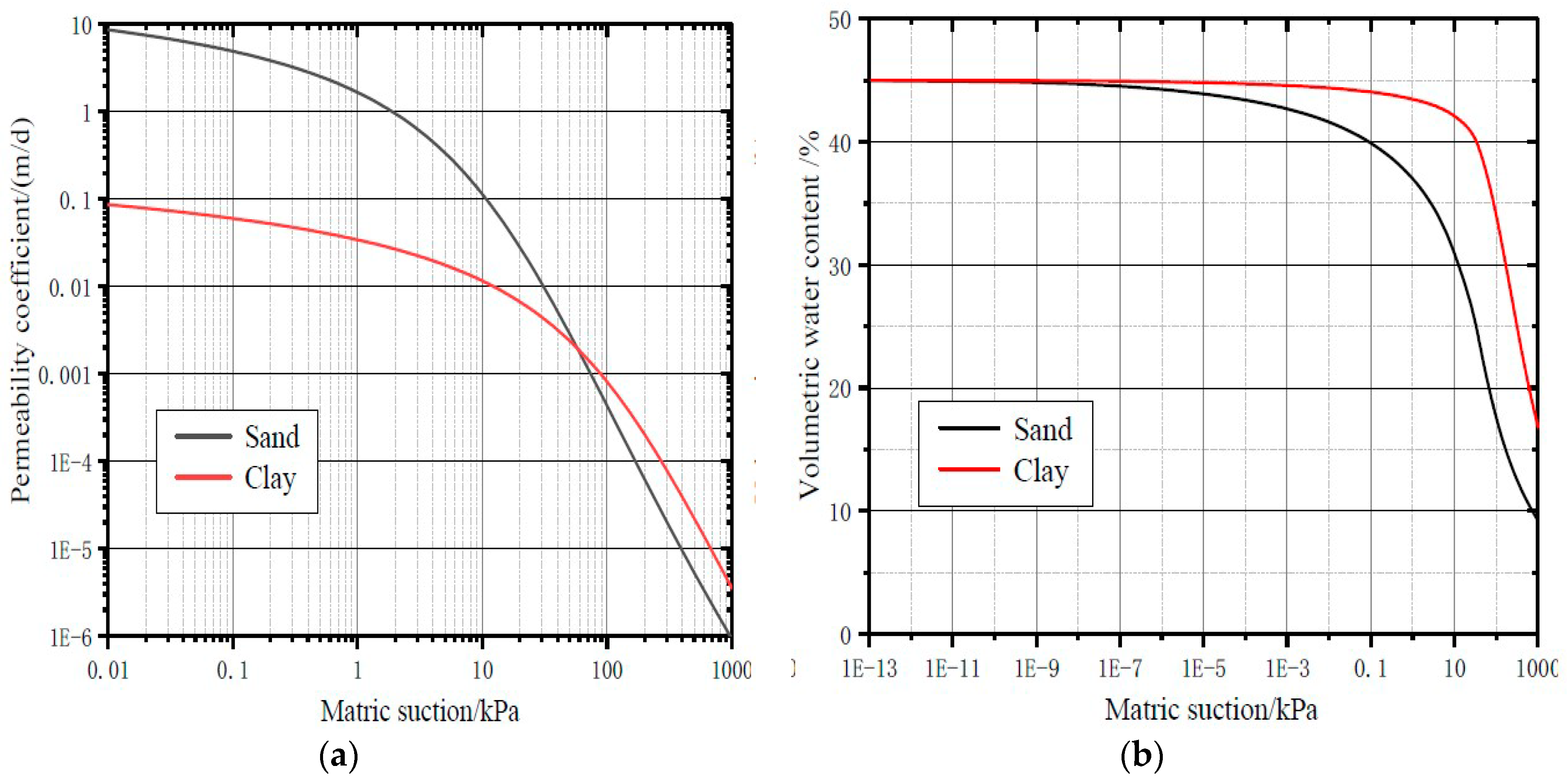
3.2. Unsaturated Soil Properties

The soil-water characteristic curves (SWCCs) adopted the Fredlund and Xing model, which can be written as [45]

$$k_w=k_s\frac{{\displaystyle \sum _{i=j}^N\frac{\Theta (e^y)-\Theta (\Psi )}{e^{y_i}}{\Theta }^{\prime }(e^{y_i})}}{{\displaystyle \sum _{i=1}^N\frac{\Theta (e^y)-{\Theta }_s}{e^{y_i}}{\Theta }^{\prime }(e^{y_i})}}$$

(7)

where k_w is the calculated conductivity for a specified water content or negative pore-water pressure; k_s is the measured saturated conductivity; Θ_s is the volumetric water content; e is the natural number 2.71828; y is a dummy variable of integration representing the logarithm of negative pore-water pressure; i is the interval between the range of j to N; j is the least negative pore-water pressure to be described by the final function; N is the maximum negative pore-water pressure to be described by the final function; Ψ is the suction corresponding to the jth interval; Θ^′ is the first derivative of the equation. Θ can be described as

$$\Theta =C\left(\Psi \right)\frac{{\Theta }_s}{{\left\{\ln \left[\mathrm{e}+{\left(\frac{\Psi }{a}\right)}^n\right]\right\}}^m}$$

(8)

where a is the air-entry value of the soil; n is a parameter that controls the slope at the inflection point in the volumetric water content function; and m is a parameter that is related to the residual water content. C(Ψ) is a correcting function defined as

$$C(\Psi )=1-\frac{\ln (1+\frac{\Psi }{C_r})}{\ln (1+\frac{\mathrm{1,000,000}}{C_r})}$$

(9)

where C_r is a constant related to the matric suction corresponding to the residual water content.

The sandy soil and clay soil were selected for analysis in this study, which represents the high and low permeability [46], as shown in Figure 3. The unsaturated parameter values are shown in

Table 1. Unsaturated parameter values.

Soil Type	SWCCs Parameters				Permeability Coefficient
	a (kPa)	m	n	θ (%)	kx (m/s)	kx (m/d)
Sand	10	1	1	45	10−4	8.64
Clay	100	1	1	45	10−6	0.0864

[47], and the SWCCs are shown in Figure 4.

3.3. Physical and Mechanics Parameters

The mechanical parameters of sand and clay were determined according to the laboratory test [47]. The Mohr–Coulomb elastoplastic criterion was applied, and the parameters are shown in

Table 2. Physical and mechanics parameters.

Soil Type	Unit Weight (kN·m−3)	Poisson’s Ratio	Elastic Modulus (GPa)	Cohesion (kPa)	Internal Friction Angle (°)
Sand	21.8	0.18	1.26	11.2	31.2
Clay	16.3	0.35	0.02	15.6	28.8

.

3.4. Definition of Anisotropy and Calculation Conditions

Previous studies mostly ignored the anisotropy ratio and direction. In fact, anisotropy widely exists in the soil, and for the hydraulic conductivity matrix [C] in Equation (2), it can be expressed as

$$[C]=\left[\begin{array}{cc}{C}_{11}& C_{12}\\ C_{21}& C_{22}\end{array}\right]$$

(10)

where C₁₁ = k_xcos²α + k_ysin²α, C₂₂ = k_xsin²α + k_ycos²α, and C₁₂ = C₂₁ = k_xsinαcosα + k_ysinαcosα. The k_x, k_y anisotropy direction α can be defined according to Figure 2; k_x is the horizontal permeability coefficient, k_y is the vertical permeability coefficient, and α is the direction between the k_y and y axes. When α = 0°, [C] is reduced to

$$[C]=\left[\begin{array}{cc}{k}_{\mathrm{x}}& 0\\ 0& k_y\end{array}\right]$$

(11)

Equation (11) is adopted in reference [39], only considering the anisotropy ratio k_r = k_x/k_y; however, the definition of anisotropy not only includes the ratio k_r but also the direction α. However, previous investigations ignored the anisotropy and especially the anisotropy direction α. The anisotropy ratio and direction can be obtained from the consolidation test of soil [32], which can be applied in the real situation.

To completely discuss the anisotropy of sandy soil and clay soil, including the anisotropy ratio k_r and the anisotropy direction α, different calculation conditions were used, as shown in

Table 3. Different calculation conditions.

Reservoir Water Drawdown Rate (m/s)	Soil Type	kx (m/s)	kr	α (°)
1.2	Sand	10−4	$\left[\begin{array}{c}1\\ 10\\ 50\\ 100\end{array}\right]$	$\left[\begin{array}{c}0\\ 15\\ 30\\ 45\\ 60\\ 75\\ 90\end{array}\right]$
	Clay	10−6	$\left[\begin{array}{c}1\\ 10\\ 50\\ 100\end{array}\right]$	$\left[\begin{array}{c}0\\ 15\\ 30\\ 45\\ 60\\ 75\\ 90\end{array}\right]$

, which includes the anisotropy ratios k_r = 1, 10, 50, and 100 and the anisotropy directions α = 0°, 15°, 30°, 45°, 60°, 75°, and 90°. The reservoir water elevation changed from 175 m to 145 m, the drawdown rate of which was 1.2 m/d. Meanwhile, the 55 d after the reservoir water level drop was also considered, and the total duration was 80 d.

4. Results

Based on the calculation conditions in Table 3, we carried out a total of 56 numerical simulations. For ease of reading, this section carries out the discussion based on the classification of sandy soil and clay soil slopes. The infiltration line, x-displacement, and safety factors of the 25th day with k_r = 10 are displayed to illustrate the influence of anisotropy direction α on seepage, deformation, and stability of the Caipo slope, and those of the 25th day with α = 45° are also displayed to show the impact of the anisotropy ratio k_r.

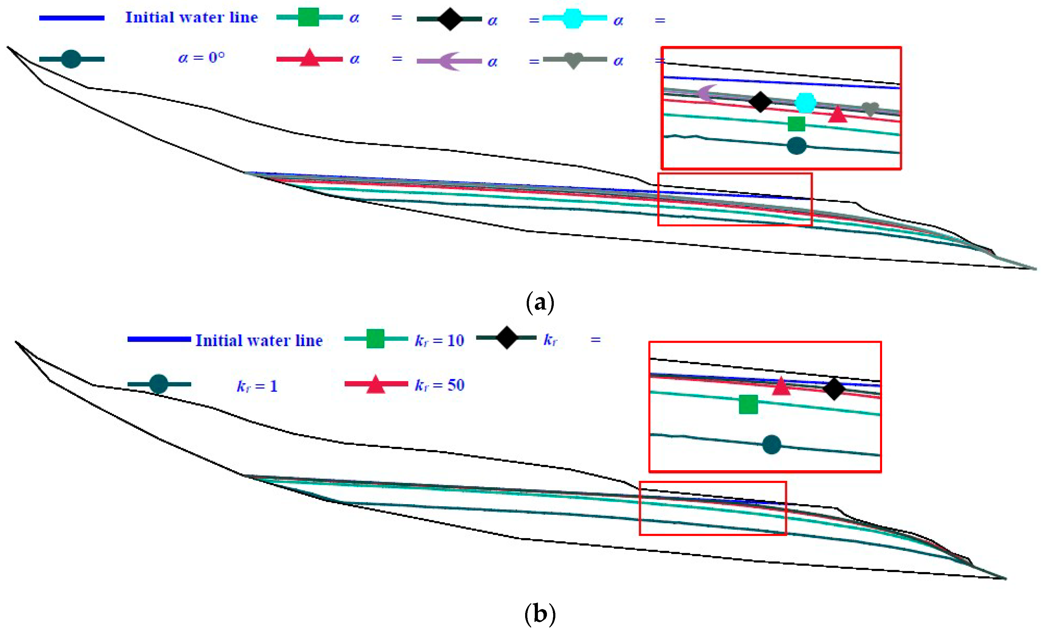
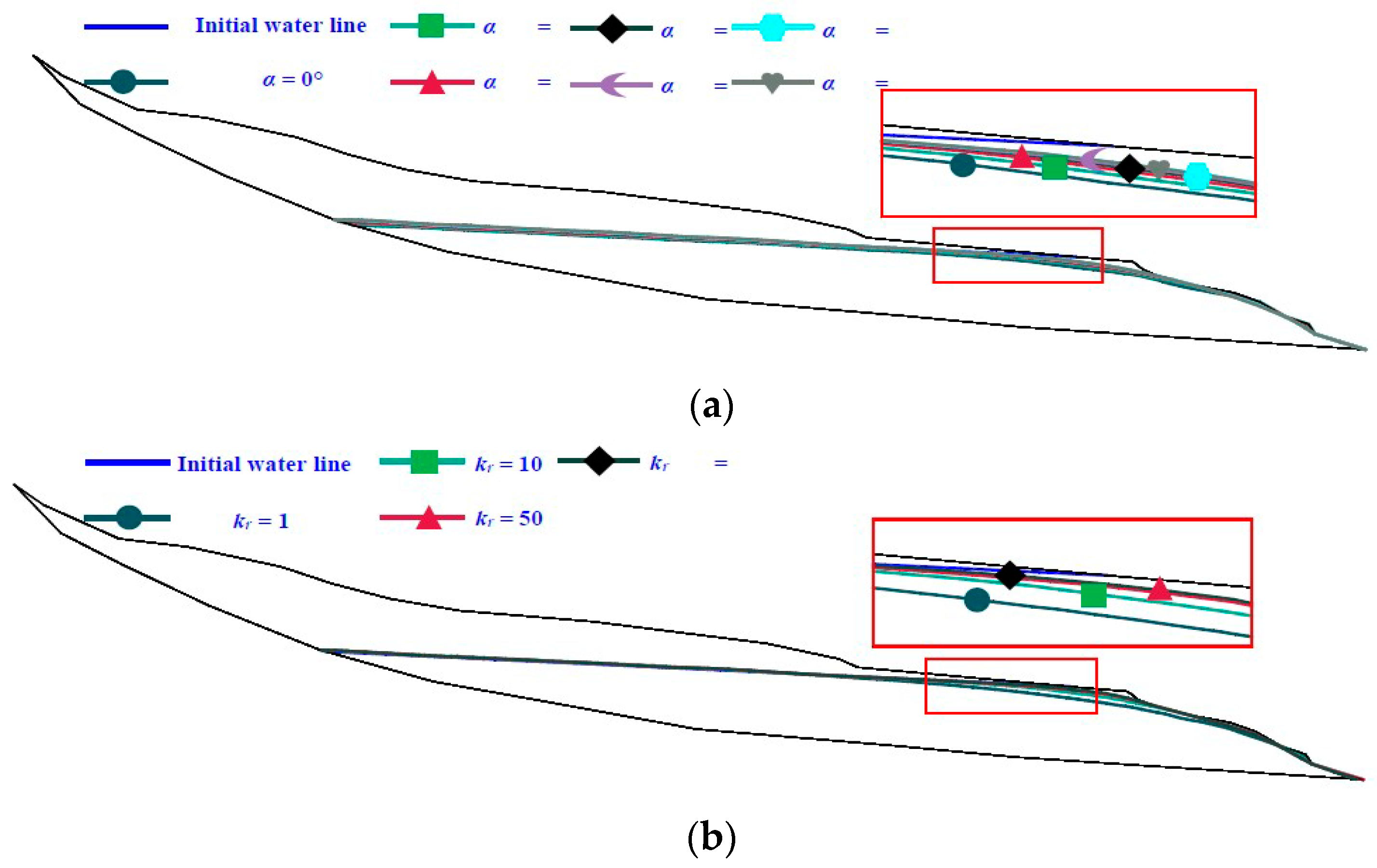
4.1. Effect of Permeability Anisotropy on Seepage Characteristics

4.1.1. Sandy Soil

The variation of infiltration lines under different permeability anisotropy degrees k_r and directions α of sandy slope is shown in Figure 5. It can be seen that there existed a delay phenomenon in the infiltration line close to the reservoir area, which means that the variation of the infiltration line lagged behind the change of reservoir water level. The anisotropy direction α had a great impact on the seepage characteristics; the infiltration line elevation increased with the increase of α, but when α was more than 45°, the elevations of different conditions were almost the same.

The anisotropy ratio k_r equally also had a significant influence on the variations of infiltration lines. With the increase of k_r, the elevation of the infiltration line increased. When k_r was larger than 50, the infiltration line of different conditions was almost the same.

4.1.2. Clay Soil

The variation of infiltration lines under different permeability anisotropy degrees k_r and directions α of clay slope is shown in Figure 6.

As can be seen from Figure 6, the infiltration line elevation of the clay slope was higher than that of the sandy slope under the same conditions. What is more, the differences under different k_r and α values were smaller than those of the sandy slope. The elevation increased with the increase of k_r and α, which was the same as the sandy slope.

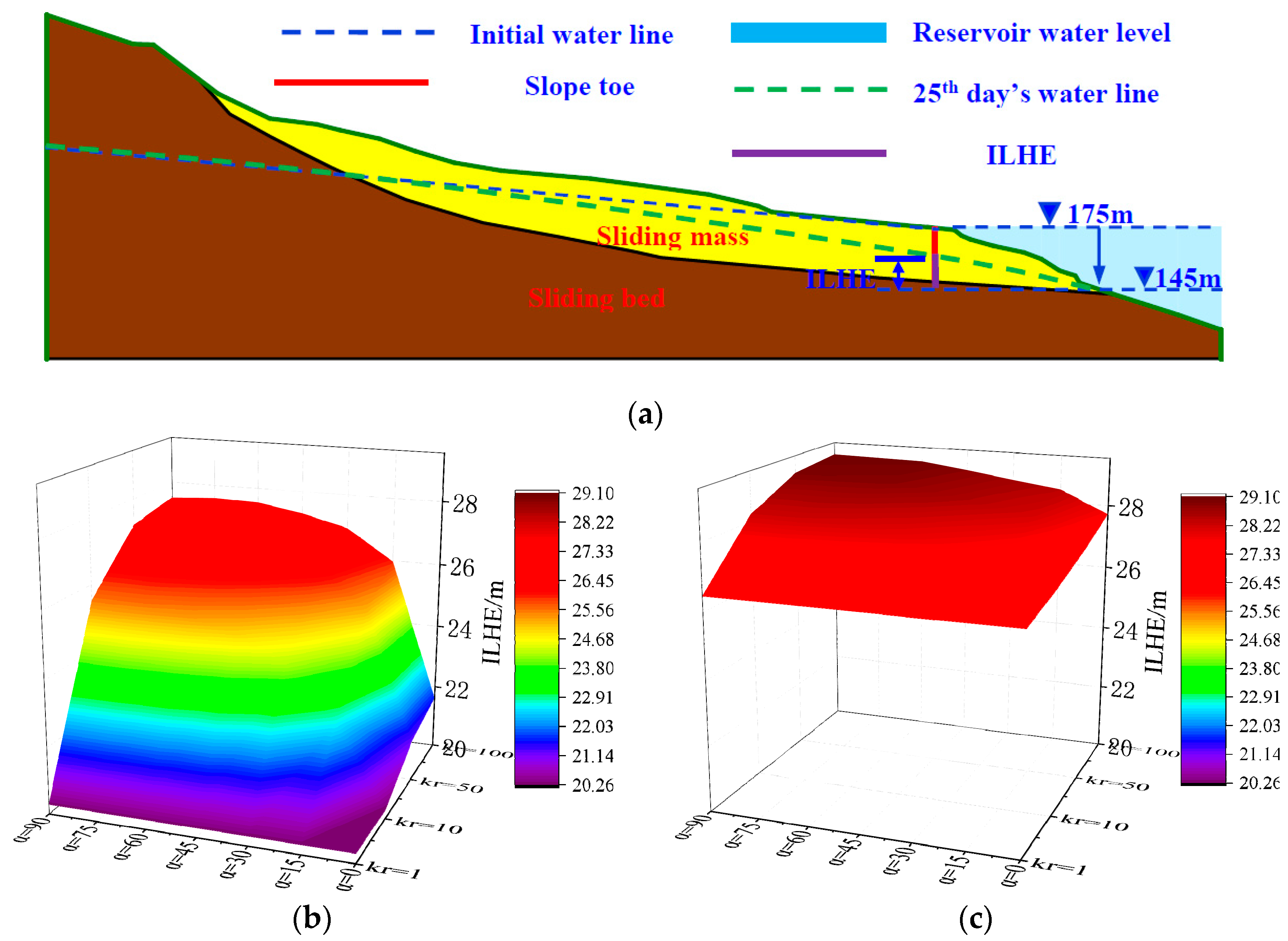
4.1.3. Analysis of Infiltration Line Hysteretic Elevation (ILHE)

It can be inferred from Section 4.1.1 and Section 4.1.2 that not only the sandy slope but also the clay slope all experienced the delay phenomenon, which led to a steep increase in the hydraulic gradient in the slope close to the reservoir area and the seepage force’s direction out of the slope, thus aggravating the instability. In order to quantitatively describe this phenomenon, the infiltration line hysteretic elevation (ILHE) was defined, as shown in Figure 7a, as the height of the intersection point between the infiltration line and the toe section of the slope to the 145 m elevation. Figure 7c show the ILHE of sandy and clay slopes, respectively, under different k_r and α values.

Generally speaking, with the increase of anisotropy ratio k_r and direction α, the ILHE of sandy and clay slopes increased to the maximum. This is because as α increased, the permeability coefficient parallel to the x axis was getting smaller and smaller for k_r > 1, and the interior water in the slope soil was more difficult to infiltrate into the reservoir, thus leading to the larger ILHE. Meanwhile, the permeability coefficient parallel to the y axis decreased with the increase of k_r, and the infiltration water line inside the slope was more difficult to draw down, which also contributed to the increase of ILHE. Compared with the clay slope, the permeability anisotropy characteristics had a greater impact on ILHE of the sandy slope. For the sandy slope, the difference between the maximum and minimum ILHE, only considering k_r, was 6.51%, which was 35.53% when considering both k_r and α. For the clay slope, the difference only considering k_r was 4.7%, which was 9.94% considering both k_r and α.

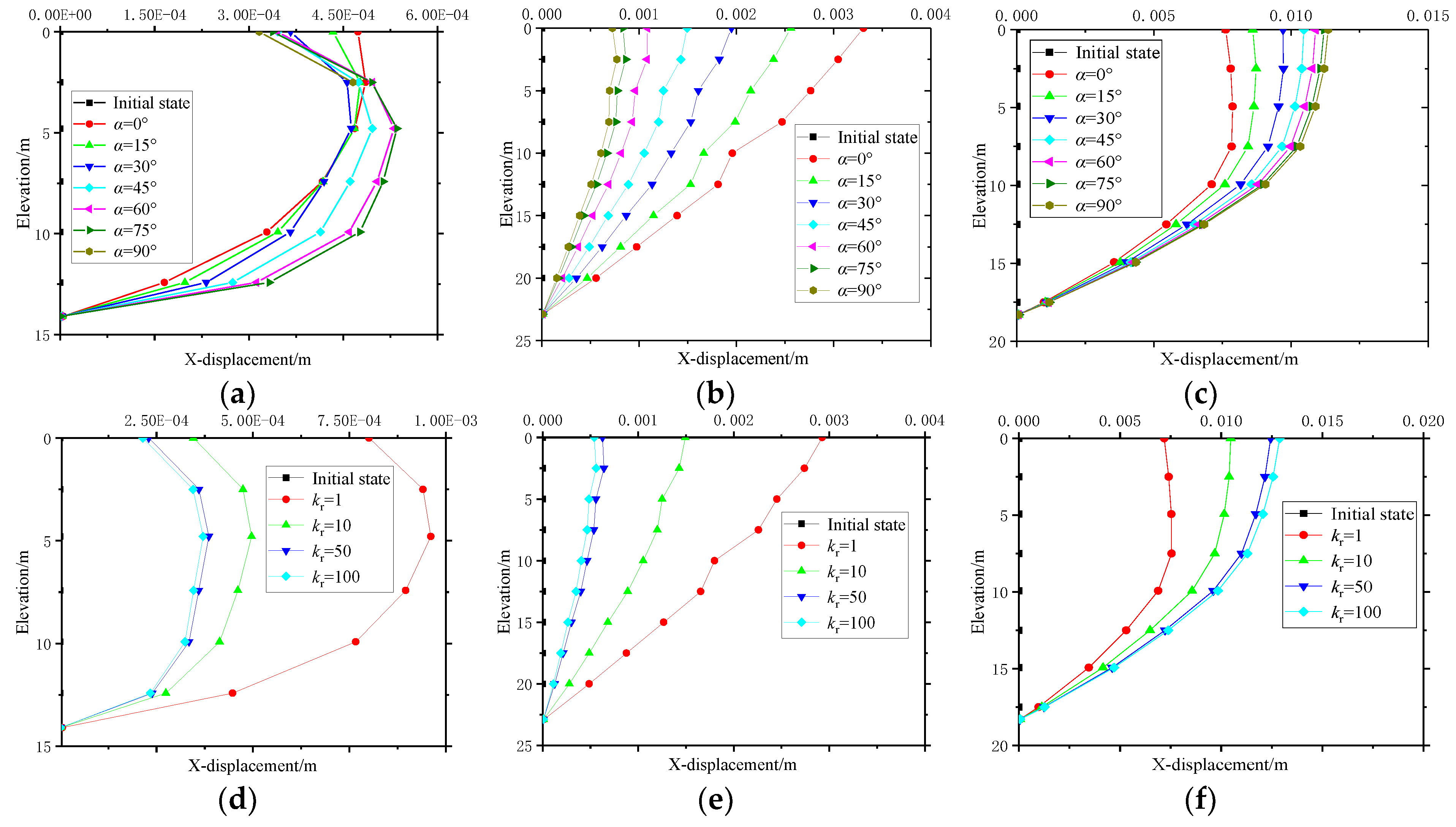
4.2. Effect of Permeability Anisotropy on DeformationCcharacteristics

4.2.1. Sandy Soil

The variations of x-displacement of the sandy slope top, slope middle, and slope toe were obtained based on the pore pressure-stress coupling method, which are shown in Figure 8.

It can be seen from the figure that the variations of x-displacement at different positions were different. For slope top, the x-displacement increased first, then decreased with the elevation. The maximum x-displacement was about 5 m from the surface. For slope middle and slope toe, the x-displacement decreased with the elevation, and the maximum x-displacement was on the slope surface. The overall x-displacement increased when the distance of the slope to the reservoir decreased, which was because the decrease of reservoir water level led to the delay phenomenon in slope soil, the most dramatic of which was the slope toe, and it caused the dynamic seepage force, which drove the slope soil to move away [6,7,8]. Therefore, we can infer that slope toe first failed with the drawdown of the reservoir water level. The permeability anisotropy characteristics also had a great impact on the variation of x-displacement. The x-displacement value of the slope top was very small compared to the slope middle and slope toe, such that it could be ignored. The x-displacement of slope middle decreased with the increase of k_r, and that of the slope toe increased with the increase of k_r. This may due to the fact that the increase of k_r and α increased the hydraulic gradient in the slope toe but decreased the hydraulic gradient in the slope middle.

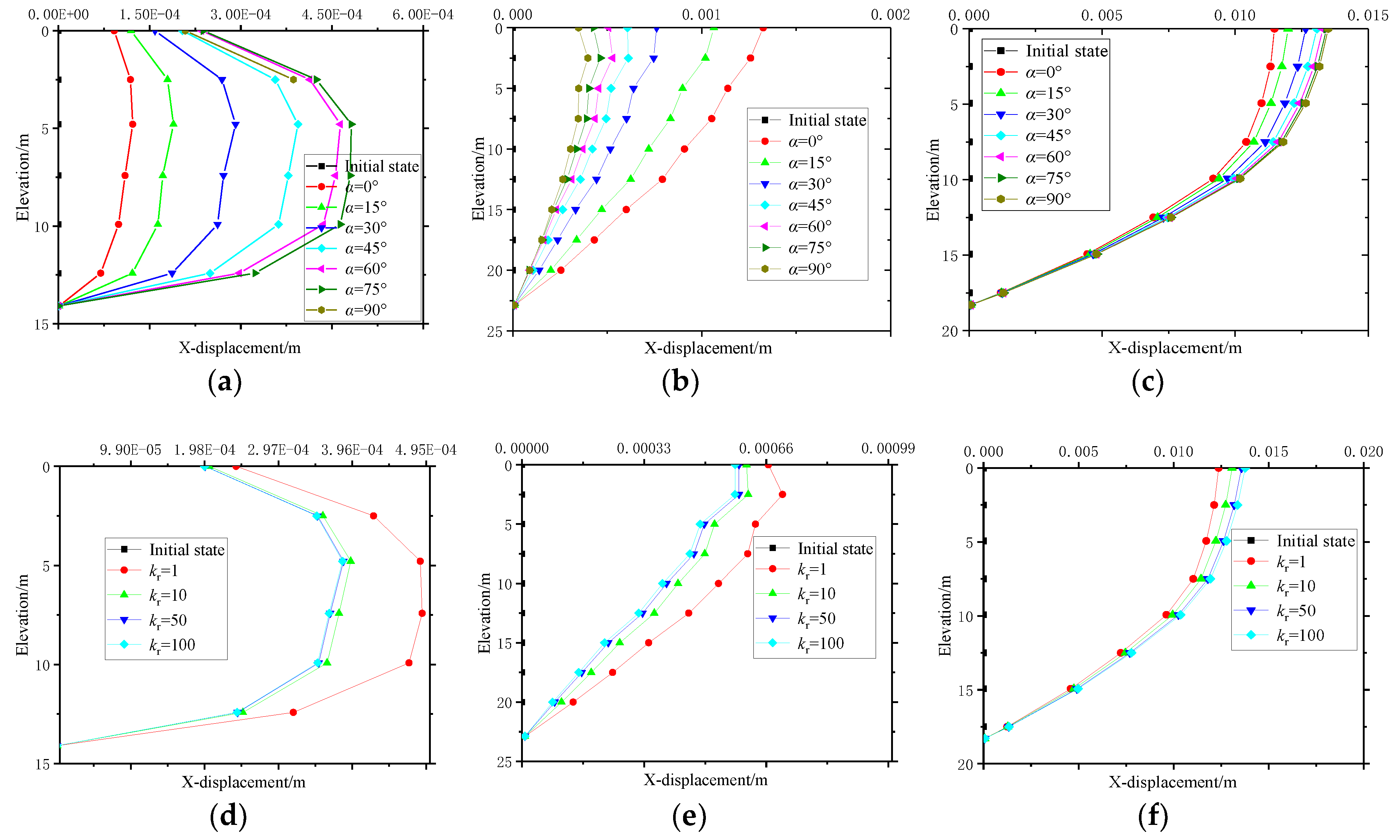
4.2.2. Clay Soil

The variations of x-displacement of clay slope top, slope middle and slope toe are shown in Figure 9.

As can be seen from Figure 9, the variations of x-displacement under different k_r and α values for clay slope were similar to those for the sandy slope. What is to be noticed is that the influence of permeability anisotropy on the clay slope was much smaller than that of the sandy slope. The x-displacement for the clay slope in the slope top and slope middle was smaller than that of the sandy slope, which was larger in the slope toe. This is easy to understand that for the clay slope, the dramatic change of infiltration line concentrated in the slope toe, but rarely changed in the slope middle and slope top. For the sandy slope, the reservoir water drawdown not only influenced the slope toe but also had some impacts on the slope middle.

4.2.3. Analysis of Maximum Horizontal Displacement (MHD)

For the purpose of quantitative study, the maximum horizontal displacement (MHD) for sandy and clay slopes under different permeability anisotropy characteristics and the variations of MHD under different conditions are shown in Figure 10.

The impact of permeability anisotropy on MHD changed with the positions of slope sections (slope top, slope middle, and slope toe). The MHD was at the maximum in the slope toe, was smaller in the slope middle, and was the smallest in the slope top. For the sandy slope, the difference between the maximum and minimum MHD, only considering k_r for the slope top, slope middle, and slope toe was 69.5%, 20.7%, and 6.9%, respectively, while it became 75.05%, 77.2%, and 21.4% for the clay slope. Taking both k_r and α into consideration, the difference was 80.0%, 94.6%, and 45.0% for the sandy slope, while it became 75.1%, 87.1%, and 32.0% for the clay slope.

4.3. Effect of Permeability Anisotropy on Safety Factors

4.3.1. Sandy Soil

The variations of safety factors (SFs) for the sandy slope under different permeability anisotropy degrees k_r and directions α are shown in Figure 11. The SF first decreased then increased with the reservoir water draw down; what should be stressed is that the permeability anisotropy not only influenced the value of the SF but also had some impact on the critical time when it reached the minimum safety factor (MSF). The SF decreased with the increase of k_r and α, which was closely related to the delay phenomenon discussed in Section 4.1. Meanwhile, the increase of k_r and α made the critical time of the MSF increase, due mainly to three reasons. One was the discharge of the water pressure acting on the slope surface, which reduced the anti-sliding force and was regarded as an unfavorable factor for slope stability. The second reason was the delay phenomenon of the infiltration line inside the slope soil, which contributed to the sharp increase in the hydraulic gradient in the slope toe and was also regarded as an unfavorable factor. The last reason was the increase of effective stress and soil strength with the decrease of infiltration line, which was regarded as a positive factor. Combined with the analysis in Section 4.1.1, the smaller the α and k_r, the more easily the interior water in the slope soil infiltrated into the reservoir, and the influence of water pressure unloading and the hydraulic gradient increase was less than the soil strength increase, which led to the earlier critical time. This was the reverse when α and k_r increased and the critical time was delayed.

4.3.2. Clay Soil

The variations of safety factors (SFs) for the clay slope under different permeability anisotropy degrees k_r and directions α are shown in Figure 12. The variations of SFs under different k_r and α values for the clay slope were different in that the SF first decreased then remained unchanged. What is more, the influence of permeability anisotropy on the clay slope was much smaller than that of the sandy slope. What is to be noticed is that the SF of the clay slope was smaller than that of the sandy slope under the same conditions, which was because of the more obvious delay phenomenon in the clay slope.

4.3.3. Analysis of Minimum Safety Factor (MSF)

The variations of MSF under different conditions are shown in Figure 13. The MSF decreased to the minimum with the increase of k_r and α. What is to be stressed is that the overall MSF of the clay slope was smaller than that of the sandy slope. The difference between the maximum and minimum MSF, only considering k_r, was 2.72% for the sandy slope, which was 9.29% for the clay slope. Taking both k_r and α into consideration, the difference was 11.58% and 12.31% for the sandy and clay slopes, respectively.

5. Discussion

5.1. Effect of Reservoir Water Level Drawdown on Seepage Deformation and Stability of Slope

Figure 14 shows the dynamic variation process of the infiltration line of the sandy slope with k_r = 1 and α = 0°, which is regarded as isotropic, as adopted by most of the previous studies. Under the action of reservoir water drawdown, the drawdown of the infiltration line lags behind that of the reservoir water level, which is due to the holding water capacity of soils. Therefore, the impact of reservoir water drawdown on the slope mainly reflects the following three aspects: (1) The delay phenomenon leads to higher pore water pressure (excess pore water pressure), which cannot be dissipated in time and forms an unsteady seepage field. The excess pore water pressure contributes to the sharp increase in the hydraulic gradient in the slope toe and is regarded as an unfavorable factor. (2) The pore pressure acting on the slope surface prevents the slope from sliding when the reservoir water level is high, but the reservoir water drawdown contributes to the unloading of the water pressure, which is also regarded as an unfavorable factor. (3) The drawdown of the reservoir water level results in the decrease of the pore water pressure interior of the slope, which increases the soil strength and the effective stress and is a positive factor. Therefore, the slope stability is affected by the above three factors, and the slope soil as well as the permeability anisotropy are important contributing factors.

Meanwhile, it is found that the x-displacement of the slope toe is the largest during the drawdown of the reservoir water level, which is also due to the delay phenomenon. In this paper, the pore pressure–stress coupling method is utilized to obtain the variation of x-displacement contour, as is shown in Figure 15a. The x-displacement in the slope toe is the largest on the 5^th day. With the further drawdown of reservoir water level, the x-displacement in the slope middle and slope top gradually gets bigger, which illustrates that the slope toe firstly fails during the reservoir water drawdown. Jiang et al. [48] conducted a series of model tests of landslides and found that the model slope failed from local slip failure to leading-edge failure under declining water levels, showing a progressive retrogressive mode, which is consist with our numerical results and verifies the correctness and rationality of the pore pressure–stress coupling method. Therefore, in the actual reservoir area landslide treatment project, we should strengthen the reinforcement measures at the slope toe of the landslide.

5.2. Effect of Permeability Anisotropy on Seepage Deformation and Stability of Slope

It is also found that the permeability anisotropy has a great influence on the seepage, deformation, and stability of the slope. Previous studies only took k_r into consideration but ignored the effect of α.

Table 4. Differences between only considering k_r and considering both k_r and α.

Analysis Content		Only Considering kr	Considering both kr and α
ILHE	Sandy slope	6.51%	35.53%
	Clay slope	4.7%	9.94%
MHD (Slope toe)	Sandy slope	6.9%	45.0%
	Clay slope	21.4%	32.0%
MSF	Sandy slope	2.72%	11.58%
	Clay slope	9.29%	12.31%

shows the statistics of the differences between only considering k_r and considering both k_r and α compared with the isotropy condition.

As can be seen from Table 4, the values of ILHE, MHD, and MSF for the sandy slope are quite different under the conditions with only considering k_r and with considering both k_r and α. Therefore, for the sandy slope, which represents the kind of soil slope with larger permeability, k_r and α must be considered in the seepage, deformation, and stability analysis. However, for the clay slope, which represents the kind of soil slope with lower permeability, the differences are much smaller. Thus, we can infer that for soil with smaller permeability, we can consider only the effect of k_r but ignore α to simplify the calculation.

5.3. Advice for Future Studies

In our analysis, the 2D model was applied to carry out the sensitivity analysis of the effect of the permeability anisotropy characteristics on the seepage, deformation, and stability of a slope, which has the advantage of simply and straightforwardly illustrating the rules. The results show that the effect of k_r and α is huge and can determine the overall slope behavior, which provides a reference for the analysis of a 3D model in real cases.

6. Conclusions

In this paper, the numerical simulation on the seepage, deformation, and stability of a slope is carried out based on the pore pressure–stress coupling model, and the Capo slope in the TGR is taken as a case study with consideration of the effect of permeability anisotropy ratio k_r and direction α, which includes the analysis of two kinds of soil type, namely a sandy slope and clay slope. The following conclusions can be drawn:

• The increase of k_r and α decreases the infiltration capacity of slope soil, which increases the pore water pressure, as well as the x-displacement, and decreases the SF. The delay phenomenon occurs during the drawdown of the reservoir water level.
• The infiltration line hysteretic elevation (ILHE), the maximum horizontal displacement (MHD), and the minimum safety factor (MSF) are defined to characterize the delay phenomenon, the deformation, and the stability. The values of ILHE, MHD, and MSF increase with the increase of k_r and α. The ILHE of the sandy slope is smaller than that of the clay slope, but the MHD and MSF of the sandy slope is larger than that of the clay slope.
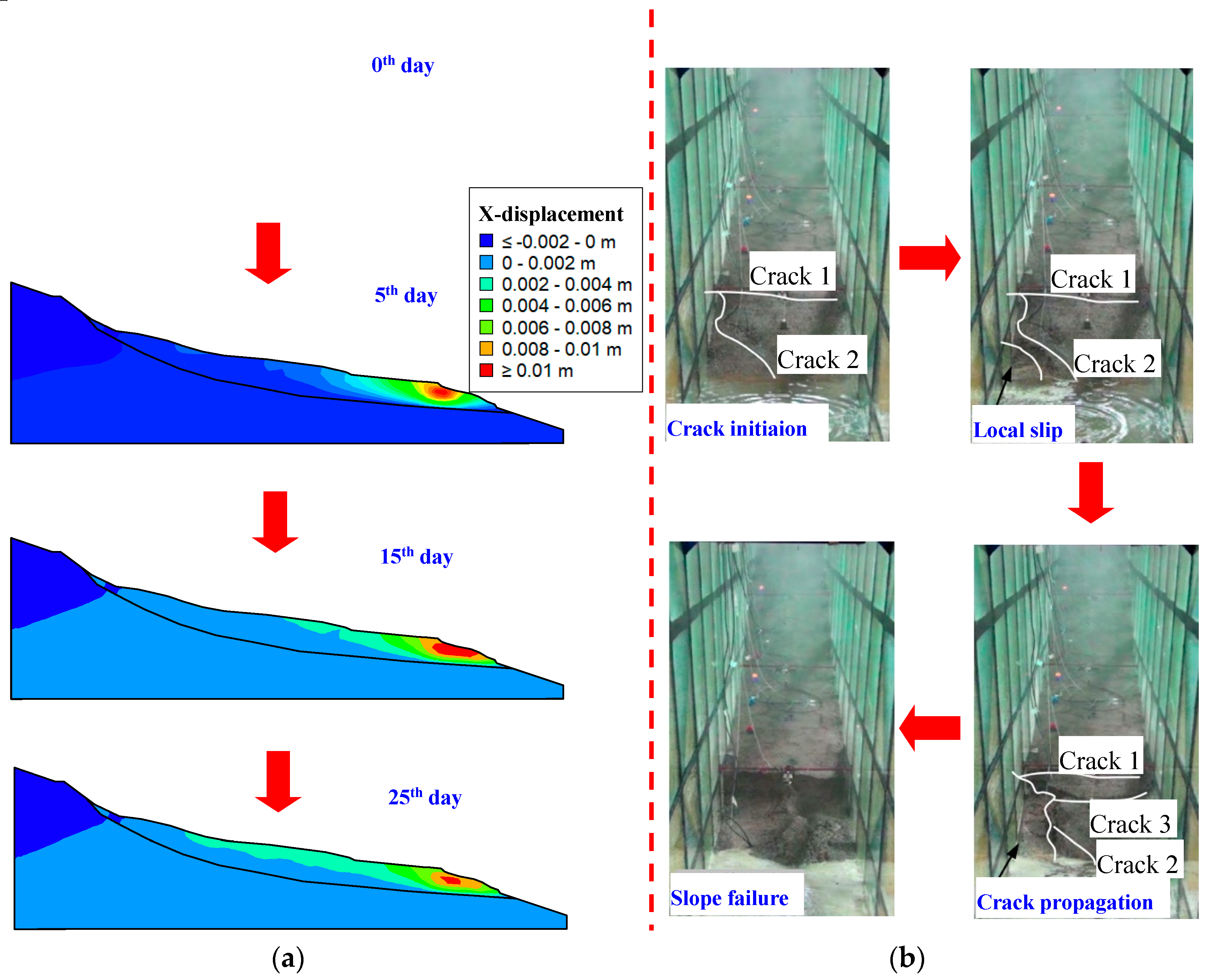
• There are mainly three aspects of the impact of reservoir water drawdown on the slope, which include two unfavorable factors containing the delay phenomenon and the water pressure unload and one positive factor containing the increase of soil strength and effective stress. The x-displacement reaches a maximum in the slope toe, which indicates the slope toe firstly fails during the reservoir water drawdown, and it is consistent with the test results in the existing literature.
• The differences of ILHE, MHD, and MSF between only considering k_r as well as both considering k_r and α are statistically analyzed. For the sandy slope, the values of ILHE, MHD, and MSF are quite different under the conditions with only considering k_r and with both considering k_r and α, while they become relatively small for the clay slope. Therefore, we must consider k_r and α for the sandy slope; however, for the clay slope, we can consider only k_r to simplify computation.
• In this paper, the permeability anisotropy ratio k_r and direction α are only considered in our simulation; future studies should combine the permeability anisotropy with the soil strength anisotropy in numerical analysis and develop new corresponding anisotropic material and carry out the model tests to verify the numerical simulation results.

References

- Li, S.; Xu, Q.; Tang, M.; Iqbal, J.; Liu, J.; Zhu, X.; Liu, F.; Zhu, D. Characterizing the spatial distribution and fundamental controls of landslides in the three gorges reservoir area, China. Bull. Eng. Geol. Environ. 2019, 78, 4275–4290. [Google Scholar] [CrossRef]
- Tang, M.; Xu, Q.; Yang, H.; Li, S.; Iqbal, J.; Fu, X.; Cheng, W. Activity law and hydraulics mechanism of landslides with different sliding surface and permeability in the Three Gorges Reservoir Area, China. Eng. Geol. 2019, 260, 105212. [Google Scholar] [CrossRef]
- Ayalew, L.; Yamagishi, H. The application of GIS-based logistic regression for landslide susceptibility mapping in the Kakuda-Yahiko Mountains, Central Japan. Geomorphology 2005, 65, 15–31. [Google Scholar] [CrossRef]
- Bi, R.; Schleier, M.; Rohn, J.; Ehret, D.; Xiang, W. Landslide susceptibility analysis based on ArcGIS and Artificial Neural Network for a large catchment in Three Gorges region, China. Environ. Earth Sci. 2014, 72, 1925–1938. [Google Scholar] [CrossRef]
- Chang, F.-J.; Chang, Y.-T. Adaptive neuro-fuzzy inference system for prediction of water level in reservoir. Adv. Water Resour. 2006, 29, 1–10. [Google Scholar] [CrossRef]
- Roeloffs, E.A. Fault stability changes induced beneath a reservoir with cyclic variations in water level. J. Geophys. Res. Space Phys. 1988, 93, 2107. [Google Scholar] [CrossRef]
- Crivelli, A.J.; Grillas, P.; Lacaze, B. Responses of vegetation to a rise in water level at Kerkini Reservoir (1982–1991), a Ramsar Site in Northern Greece. Environ. Manag. 1995, 19, 417–430. [Google Scholar] [CrossRef]
- Li, S.; Knappett, J.A.; Feng, X. Centrifugal test on slope instability influenced by rise and fall of reservoir water level. Chin. J. Rock Mech. Eng. 2008, 27, 1586–1593. [Google Scholar]
- Zhou, C.; Yin, K.; Cao, Y.; Ahmed, B. Application of time series analysis and PSO–SVM model in predicting the Bazimen landslide in the Three Gorges Reservoir, China. Eng. Geol. 2016, 204, 108–120. [Google Scholar] [CrossRef]
- Huang, D.; Gu, D.-M.; Chen, Z.-Q.; Zhu, H.; Chen, C.-J. Hybrid effects of rainfall and reservoir level fluctuation on old Taping H2 landslide in Wushan County in Three Gorges Reservoir area. Chin. J. Geotech. Eng. 2017, 39, 2203–2211. [Google Scholar]
- Li, Z.; He, Y.-J.; Sheng, J.-B.; Li, H.-E.; Yang, Y. Landslide model for slope of reservoir bank under combined effects of rainfall and reservoir water level. Chin. J. Geotech. Eng. 2017, 39, 452–459. [Google Scholar]
- Wang, H.; Sun, Y.; Tan, Y.; Sui, T.; Sun, G. Deformation characteristics and stability evolution behavior of Woshaxi landslide during the initial impoundment period of the Three Gorges reservoir. Environ. Earth Sci. 2019, 78, 592. [Google Scholar] [CrossRef]
- Iqbal, J.; Tu, X.; Gao, W. The Impact of Reservoir Fluctuations on Reactivated Large Landslides: A Case Study. Geofluids 2019, 2019, 1–16. [Google Scholar] [CrossRef]
- Yan, L.; Xu, W.; Wang, H.; Wang, R.; Meng, Q.; Yu, J.; Xie, W.-C. Drainage controls on the Donglingxing landslide (China) induced by rainfall and fluctuation in reservoir water levels. Landslides 2019, 16, 1583–1593. [Google Scholar] [CrossRef]
- Luo, F.; Zhang, G. Progressive failure behavior of cohesive soil slopes under water drawdown conditions. Environ. Earth Sci. 2016, 75, 973. [Google Scholar] [CrossRef]
- Hu, X.; He, C.; Zhou, C.; Xu, C.; Zhang, H.; Wang, Q.; Wu, S. Model Test and Numerical Analysis on the Deformation and Stability of a Landslide Subjected to Reservoir Filling. Geofluids 2019, 2019, 1–15. [Google Scholar] [CrossRef] [Green Version]
- Yang, C.-B.; Zhu, B.; Kong, L.-G.; Han, L.-B.; Chen, Y.-M. Centrifugal model tests on failure of silty slopes induced by change of water level. Chin. J. Geotech. Eng. 2013, 35, 1261–1271. [Google Scholar]
- Hu, X.; Tang, H.; Li, C.; Sun, R. Stability of Huangtupo riverside slumping mass II# under water level fluctuation of Three Gorges Reservoir. J. Earth Sci. 2012, 23, 326–334. [Google Scholar]
- Jian, W.; Xu, Q.; Yang, H.; Wang, F. Mechanism and failure process of Qianjiangping landslide in the Three Gorges Reservoir, China. Environ. Earth Sci. 2014, 72, 2999–3013. [Google Scholar] [CrossRef]
- Song, K.; Yan, E.; Zhang, G.; Lu, S.; Yi, Q. Effect of hydraulic properties of soil and fluctuation velocity of reservoir water on landslide stability. Environ. Earth Sci. 2015, 74, 5319–5329. [Google Scholar] [CrossRef]
- Huang, F.; Luo, X.; Liu, W. Stability Analysis of Hydrodynamic Pressure Landslides with Different Permeability Coefficients Affected by Reservoir Water Level Fluctuations and Rainstorms. Water 2017, 9, 450. [Google Scholar] [CrossRef] [Green Version]
- Ye, C.; Li, S.; Zhang, Y.; Zhang, Q. Assessing soil heavy metal pollution in the water-level-fluctuation zone of the Three Gorges Reservoir, China. J. Hazard. Mater. 2011, 191, 366–372. [Google Scholar] [CrossRef]
- Naselli-Flores, L.; Barone, R. Importance of water-level fluctuation on population dynamics of cladocerans in a hypertrophic reservoir (Lake Arancio, south-west Sicily, Italy). Hydrobiologia 1997, 360, 223–232. [Google Scholar] [CrossRef]
- Bao, Y.; Gao, P.; He, X. The water-level fluctuation zone of Three Gorges Reservoir—A unique geomorphological unit. Earth-Sci. Rev. 2015, 150, 14–24. [Google Scholar] [CrossRef]
- William, R.J. Control of Biomphalaria Glabrata in a Small Reservoir by Fluctuation of the Water Level. Am. J. Trop. Med. Hyg. 1970, 19, 1049–1054. [Google Scholar]
- Wu, L.M.; Wang, Z.Q. Three Gorges Reservoir Water Level Fluctuation Influents on the Stability of the Slope’s Analysis. Adv. Mater. Res. 2013, 739, 283–286. [Google Scholar] [CrossRef]
- Zhang, X.; Tan, Z.; Zhou, C. Seepage and stability analysis of landslide under the change of reservoir water levels. Chin. J. Rock Mech. Eng. 2016, 35, 713–723. [Google Scholar]
- Jiao, Y.-Y.; Song, L.; Tang, H.-M.; Li, Y.-A. Material Weakening of Slip Zone Soils Induced by Water Level Fluctuation in the Ancient Landslides of Three Gorges Reservoir. Adv. Mater. Sci. Eng. 2014, 2014, 1–9. [Google Scholar] [CrossRef] [Green Version]
- Tan, S.D.; Wang, Y.; Zhang, Q.F. Environmental challenges and countermeasures of the water-level-fluctuation zone (WLFZ) of the Three Gorges Reservoir. Resour. Environ. Yangtze Basin 2008, 17, 101–105. [Google Scholar]
- Xiang, L.; Wang, S.; Wang, L. Response of Typical Hydrodynamic Pressure Landslide to Reservoir Water Level Fluctuation: Shuping Landslide in Three Gorges Reservoir as an Example. J. Eng. Geol. 2014, 22, 876–882. [Google Scholar]
- Hu, H.; Li, Y.; Li, H.; Hu, K.-F.; Zheng, D.-B. Analytic Solutions and Their Errors of Groundwater Phreatic Line in Bank Slope under Reservoir Water Level Fluctuation. J. Yangtze River Sci. Res. Inst. 2013, 30, 44–48. [Google Scholar]
- Song, Y.-Q.; Wu, C.; Ye, G. Permeability and anisotropy of upper Shanghai clays. Rock Soil Mech. 2018, 39, 2139–2144. [Google Scholar]
- Wang, T.-H.; Yang, T.; Lu, J. Influence of dry density and freezing-thawing cycles on anisotropic permeability of loess. Rock Soil Mech. 2016, 37, 72–78. [Google Scholar]
- Todd, D. Groundwater Hydrology; Jon Wiley & Sons Inc.: New York, NY, USA, 1980; p. 103. [Google Scholar]
- Yuan, J.-P.; Lin, Y.-L.; Ding, P.; Han, C.-L. Influence of anisotropy induced by fissures on rainfall infiltration of slopes. Chin. J. Geotech. Eng. 2016, 38, 76–82. [Google Scholar]
- Yuan, J.-P.; Lin, Y.-L.; Ding, P.; Han, C.-L. Coupling analysis of seepage-damage-fracture in fractured rock mass and engineering application. Chin. J. Geotech. Eng. 2010, 32, 24–32. [Google Scholar]
- Mahmood, K.; Ryu, J.H.; Kim, J.M. Effect of anisotropic conductivity on suction and reliability index of unsaturated slope exposed to uniform antecedent rainfall. Landslides 2013, 10, 15–22. [Google Scholar] [CrossRef]
- Dong, J.J.; Tu, C.H.; Lee, W.R.; Jheng, Y.-J. Effects of hydraulic conductivity/strength anisotropy on the stability of stratified, poorly cemented rock slopes. Comput. Geotech. 2012, 40, 147–159. [Google Scholar] [CrossRef]
- Yeh, H.F.; Tsai, Y.J. Analyzing the Effect of Soil Hydraulic Conductivity Anisotropy on Slope Stability Using a Coupled Hydromechanical Framework. Water 2018, 10, 905. [Google Scholar] [CrossRef] [Green Version]
- Li, X.F. Study on seepage Stability of Caipo Reservoir under combined rainfall condition. J. Water Resour. Water Eng. 2019, 30, 155–160. [Google Scholar]
- Simon, A.; Collison, A.J.C. Quantifying the mechanical and hydrologic effects of riparian vegetation on streambank stability. Earth Surf. Process. Landf. 2002, 27, 527–546. [Google Scholar] [CrossRef]
- Ni, J.J.; Leung, A.K.; Ng, C.W.W.; Shao, W. Modelling hydro-mechanical reinforcements of plants to slope stability. Comput. Geotech. 2018, 95, 99–109. [Google Scholar] [CrossRef]
- Ng, C.W.W.; Leung, A.; Ni, J. Plant–Soil Slope Interaction; CRC Press: Boca Raton, FL, USA, 2019. [Google Scholar] [CrossRef]
- GEO-SLOPE International Ltd. Seepage Modeling with SEEP/W 2007; Geo-Slope International Ltd.: Calgary, AB, Canada, 2010. [Google Scholar]
- Fredlund, D.G.; Rahardjo, H. Soil Mechanics for Unsaturated Soils; Wiley: Hoboken, NJ, USA, 1993. [Google Scholar]
- Liu, J.; Zen, L.; Fu, H.Y.; Shi, Z.N.; Zhang, Y.J. Variation law of rainfall infiltration depth and saturation zone of soil slope. J. Cent. South Univ. (Sci. Technol.) 2019, 50, 452–459. [Google Scholar]
- Tang, D.; Li, D.Q.; Zhou, C.B.; Phoon, K.-K. Slope stability analysis considering antecedent rainfall process. Rock Soil Mech. 2013, 34, 3239–3248. [Google Scholar]
- Jiang, Q.Q.; Jiao, Y.Y.; Song, L.; Wang, H.; Xie, B.T. Experimental study on reservoir landslide under rainfall and water-level fluctuation. Rock Soil Mech. 2019, 40, 4361–4370. [Google Scholar]