Cost–Benefit Analysis of Leakage Reduction Methods in Water Supply Networks

Department of Built Environment, Aalto University, P.O. Box 15200, 00076 Aalto, Finland
*
Author to whom correspondence should be addressed.
Water 2020, 12(1), 195; https://doi.org/10.3390/w12010195
Submission received: 16 December 2019
/
Revised: 4 January 2020
/
Accepted: 7 January 2020
/
Published: 10 January 2020
(This article belongs to the Special Issue Management of Urban Water Services)
Abstract
:Reducing water loss from water supply systems is often regarded as one of the most important ways to improve the resource efficiency of water supply services. However, the costs and impacts of water loss reduction efforts need to be weighed against the benefits to define the optimal water loss target level. To this end, we conducted a cost–benefit analysis of three investment-based leakage reduction methods: district metering, pressure reduction, and pipe renovations. Furthermore, we conducted uncertainty and sensitivity analysis to determine the most relevant data for leakage analysis and policymaking on a national level. The results indicate that water loss management might not be directly cost-beneficial to utilities operating with moderate leakage levels. Neither leakage percentage nor the Infrastructure Leakage Index (ILI) were suitable for leakage target setting for the Finnish utilities. The costs of investing in district metering or renovations were the most influential factors in the sensitivity analysis, but the results showed that the estimated values were sufficiently accurate for assessing leakage policies.
1. Introduction
Reducing water loss is one of the most important ways to improve the resource efficiency of water supply services. Globally, water loss amounts to 126 billion cubic meters per year (expressed as non-revenue water) with an estimated value of USD 39 billion per year [1]. Besides the societal and environmental issues of water scarcity, water availability, and energy consumption, leakage in water distribution systems can cause technical problems for the water providers. A high level of leakage is usually linked with aged infrastructure, and thus it is linked with a higher rate of pipe bursts. Bursts and leaks in the network affect its reliability, service continuity, and risk of contamination. Moreover, operating and modeling the network accurately and reliably is more difficult if there is a lot of leakage.
Water loss from water supply networks is often classified as background leakage and leakage from bursts [2]. The background leakage typically includes flow from deficient joints and small defects in the pipe walls, while the burst-related leakage includes outflow from larger, usually detectable holes and cracks. In general, leakage can be reduced by localizing, pinpointing, and repairing the detectable leaks, by reducing the hydraulic pressure and by renovating pipelines [2,3].
Identifying the areas with higher leakage levels and possible detectable leaks can be achieved through so-called district metering, wherein flow and pressure measurement stations are set at the boundaries of enclosed areas in the network. While these network measurements can be used to find detectable leaks, background leakage can mainly be reduced by lowering the hydraulic pressure or by renovating pipelines. The pressure in the pipe network affects all the demand components, including leakage, since the water outflow rate is a function of pressure. Pressure management has been considered to be one of the most efficient methods for controlling leakage, especially background leakage [4,5]. Renovating pipelines, on the other hand, has other considerable benefits besides cutting down on water loss, such as reducing large pipe bursts and improving the network reliability.
All of the leakage mitigation methods mentioned above consume some resources, which is why they need to be weighed against their benefits. Some leakage appraisal methods presented in the literature include the sustainable economic level of leakage (SELL) framework [6], cost–benefit analysis case studies [7,8], and economic inefficiency measures [9,10,11]. Malm et al. [8] presented a comparison of the costs and benefits of four different leakage control alternatives against a predetermined leakage target. The case study distribution system benefited the most from increased leak detection efforts, either through increasing personnel or through investments in district metering. Another case study [12], in the absence of detailed data, used the active leakage control cost curve model developed within the SELL framework, which is only applicable to a short-run situation as opposed to long-term investments. In Portugal, Martins et al. [9] found some indication that the unit cost of water (including all costs of supplying water) could be lowered by reducing leakage, but the study did not indicate any specific methods for leakage control. In Chile, the results suggested that costs could not be saved by active leakage management [10].
In the light of these somewhat contradictory results, more information is needed for the optimization of leakage management on a policy level as well as for investment planning. We present a formula for estimating the leakage reduction potential of Finnish water utilities. We conduct cost–benefit analysis to estimate the economic level of leakage of these utilities. We analyze the uncertainty and sensitivity of the input variables to specify which data are the most relevant for leakage analysis and policymaking. The leakage reduction methods in the analysis are district metering, pressure control, and pipe renovations.
2. Materials and Methods
We calculated and analyzed the net present value (NPV) of three investment-based leakage reduction measures: (1) district metering areas, (2) district metering areas with pressure reduction, and (3) renovations. Net present value (NPV) [13] is often used to estimate the value of investments and other capital projects with cash flows occurring over time. The yearly cash flow is discounted to present value as
where r = discount rate, T = total time in years, t and Rt = cash flow in year t.
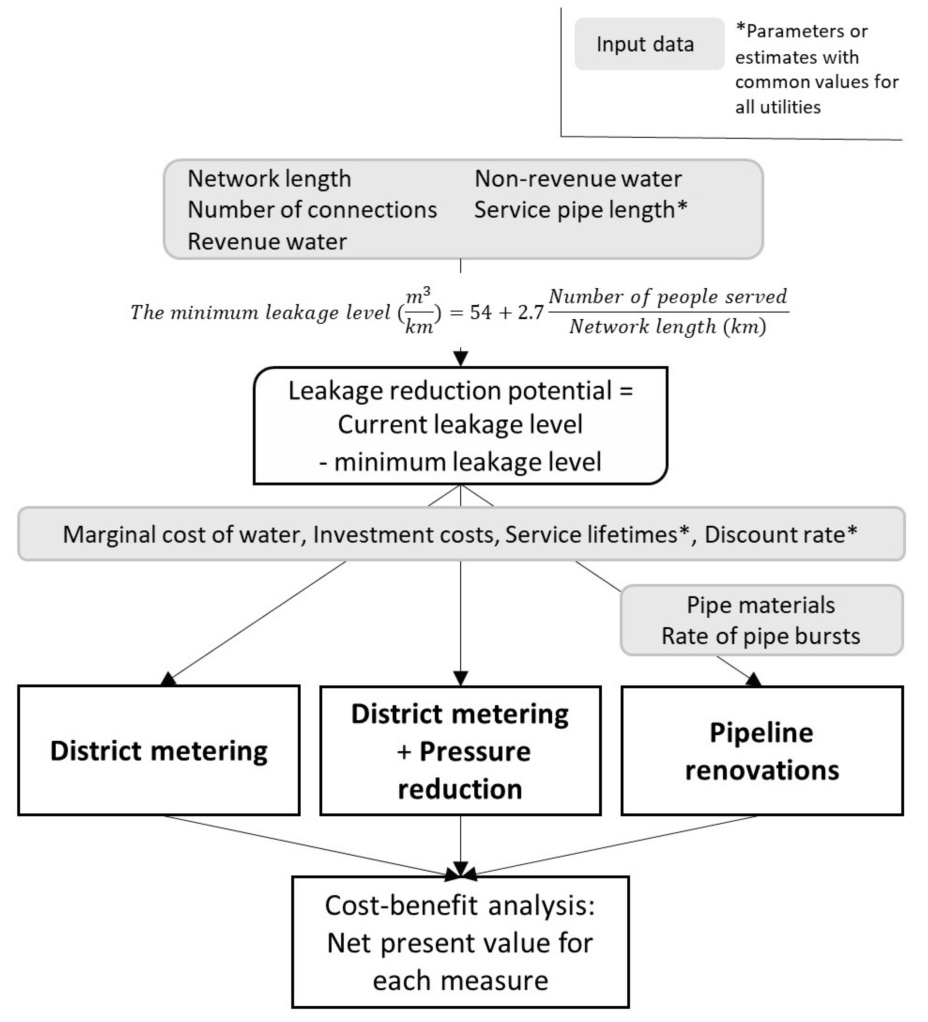
First, we calculated the leakage reduction potential of each utility. Next, we calculated the NPVs based on the direct costs and benefits acquired by the utilities. The costs are calculated as a one-time investment, while future benefits (reduced water loss and bursts) are discounted for the whole lifetime of each measure. The overview of the workflow along with the input data is presented in Figure 1.
2.1. Data
Our dataset contains 92 water utilities from Finland, covering 29% of all municipalities, 38% of the total network length, and 70% of those inhabitants of Finland that are served by centralized water supply. The smallest utility serves around 3300 people, and the largest serves 1,112,000 people.
The Finnish environmental administration’s water utility information system (VEETI, [14]) sourced the following data: (1) volume of water pumped into the network, (2) billed volume, (3) the network length for different pipe material groups (metal, plastic, and other/unknown), (4) number of people served, (5) number of connections, (6) number of pipe failures per year, (7) energy consumption in water treatment and distribution, and (8) raw water source (surface water, groundwater, or artificial groundwater).
The average energy consumption was 0.75 kWh/m3 for surface water facilities, 0.56 kWh/m3 for groundwater facilities, and 0.22 kWh/m3 for water distribution. The average values were used for the around 60% of the utilities that did not report energy consumption. The cost of energy was estimated as electricity cost, even though a small part of the total energy consumption sometimes comes from other sources such as fuel oil. The cost of electricity was estimated based on the Finnish electricity price statistics [15] and was 0.07–0.12 euros/kWh. The unbilled authorized consumption was assumed to be 2% of the network input for all utilities. The average length of service lines was set to 22.5 m [16]. All customers, usually the property owner, are metered in Finland, and the water meters are located inside the buildings.
Water Supply in Finland
Finland has a population of about 5.5 million people, of whom 92% are connected to some centralized drinking water supply. Drinking water services are mainly provided by municipally-owned utilities. The total length of water distribution pipes in the country is around 107,000 km, most of which was built after 1970 [17]. There is no water scarcity on the average year, although some basins may experience water stress during drought episodes [18]. Water demand per person has been decreasing in the last decades, but urbanization may lead to increases in the total water demand in some cities. According to our estimation, around 11% of all municipalities will face increases in water demand over the next 20 years.
2.2. Estimating the Leakage Reduction Potential
We formulated the leakage reduction potential as the difference between the current leakage level and the theoretically minimum leakage level, which was based on leakage per pipe length and the customer density. Since larger cities have larger pipes and more service connections per pipe length, leakage per pipe length is also higher. The density of people per pipe length was chosen as the indicator for this variability.
Originally, we wanted to use the formula for the unavoidable annual real losses (UARL) [22] as the theoretical minimum leakage level, but it was discarded because over half of the utilities had a current leakage level less than the UARL. Thus, instead, we drafted a formula following the current lowest leakage levels as
We compared this formulation to the UARL, which is given by
where Lm = length of mains (km), Nc = number of service connections, Ls = total length of service pipes (km), and h = average pressure head (m). The UARL can be used with the current leakage level to calculate the infrastructure leakage index (ILI) as
where CARL = the current annual real losses and UARL = the unavoidable annual real losses [22]. Thus, a utility has leakage reduction potential if the ILI is over one.
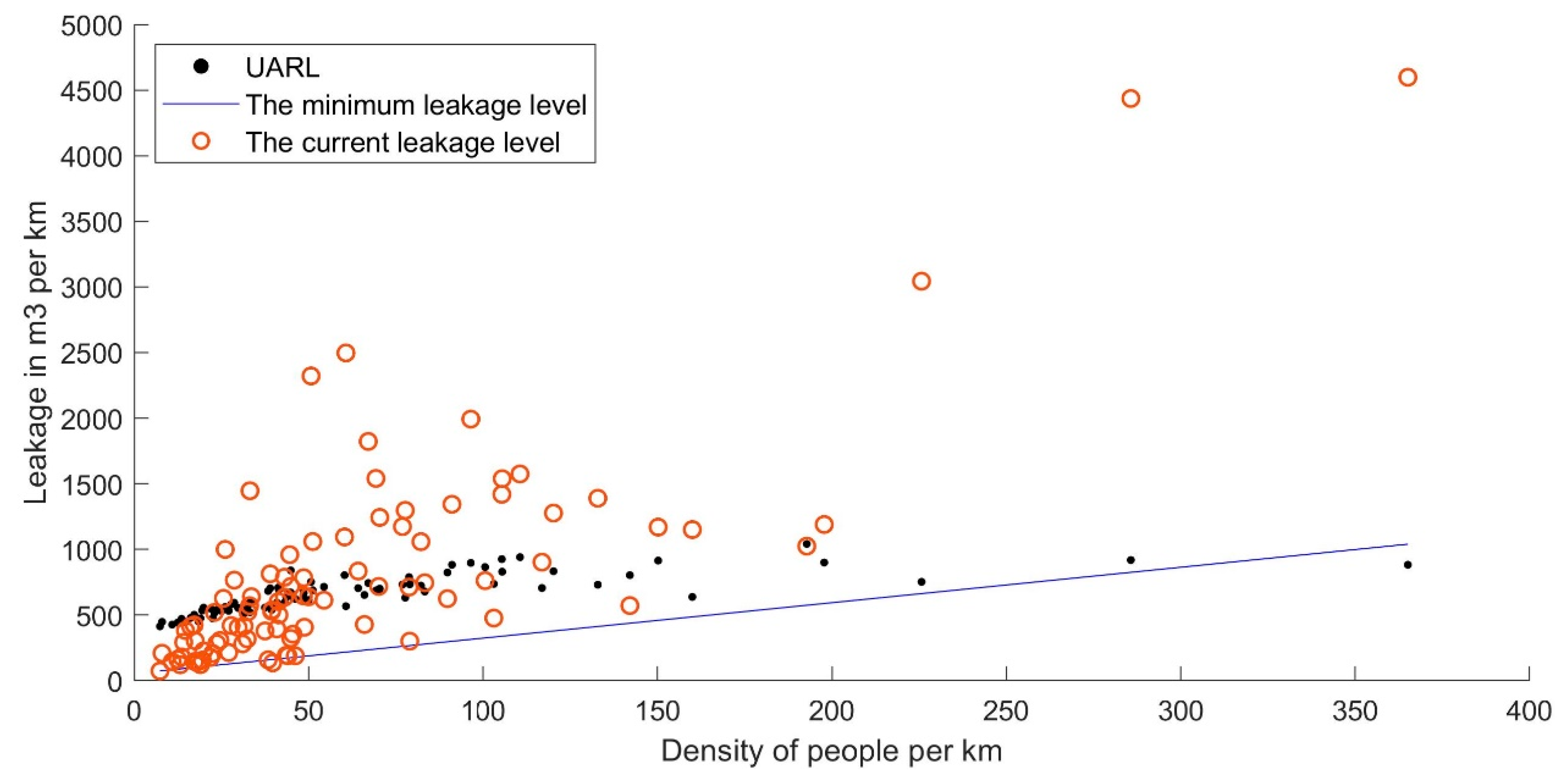
Figure 2 shows the formulation of the minimum leakage level compared to the current leakage levels and the UARL of each utility.
2.3. The Leakage Reduction Methods
We included district metering, district metering with pressure reduction, and renovations as leakage reduction methods. All of these measures have the potential to reduce leakage, and renovations also reduce pipe failures. The costs of the measures for the water utility include direct construction and management costs. The benefits include the avoided cost of leakage and the avoided cost of pipe failure repairs, including the repair cost and damages paid by the utility. The cost of leakage was calculated as the marginal cost of water, which is the cost of producing and distributing one (more) unit of water, including power (energy) and treatment chemicals. We calculated the net present value of each leakage reduction method with a discount rate of 3.5%.
2.3.1. District Metering
District metered areas (DMAs) allow utilities to follow water loss levels on fixed areas. The districts are created by closing valves or connections and metering the flow on the remaining connections at the area boundaries. This helps in detecting leaks, thus reducing water loss by reducing the run time of unreported leaks. We assumed that the leakage reduction potential of a DMA system is 30% of the total leakage reduction potential, based on the value used by Malm et al. [8] in Sweden.
The variables associated with the DMAs were selected based on a construction plan of a DMA system for a Finnish utility. The average DMA size was set to 560 service connections, but all utilities with over 800 service connections had a minimum of two DMAs. This yielded DMAs with pipe lengths between 16 km and 361 km. The cost per DMA was set to 48,000 euros with an average of 2.7 metering stations per DMA. The lifetime (depreciation period) of the metering stations was assumed to be 20 years.
2.3.2. Pressure Reduction
The network pressure affects both leakage level and water use, both of which can be modeled as flow through an opening (orifice). The outflow through an orifice is a function of the pressure head, orifice area, gravitational acceleration, and orifice attributes. In elastic pipes, the area of an opening can change along with changes in pressure, which needs to be taken into account [23]. We used the empirical leakage-pressure relationship
where L0 = initial leakage volume, L1 = leakage volume after pressure change, P0 = initial pressure, P1 = pressure after change, and N1 = empirical exponent for the leakage–pressure relationship [24]. Based on previous assessments, values of 1.5 and 0.5 for the N1 exponent are often assumed for elastic and rigid materials, respectively [25]. We used the following values: ‘plastic’ N1 = 1.5, ‘other/unknown’ N1 = 1, and ‘metal’ N1 = 0.5.
In the water user side, the N1 exponent has usually much lower values, because the water user controls the flow through faucets and shower heads and may increase the flow, for example during a shower, if pressure and flow are decreased. Not much literature could be found with measured values for the N1 exponent in relation to water use and pressure. For the water use–pressure relationship, we used Equation (5) with N1 exponent value of 0.15, which has been reported for office buildings in the Czech Republic [26].
The network pressure levels were not known, and thus an average pressure of 50 m and an average potential pressure reduction of 5 m were assumed for all utilities. The pressure change was assumed to cause no significant changes in pipe failure frequencies, because the pressure–burst relationship is not yet well understood [5]. Pressure reduction was assumed to be carried out within the DMAs. Half of the DMAs were assumed to be suitable for pressure reduction with an average of 2.7 pressure-reducing valves (PRV) installed per area. This means that half of the areas would have an average pressure reduction of 10 m and half would not have any pressure reduction. The average cost of a pressure-reducing valve was set to 9000 euros (based on Gomes et al. [4]), and the lifetime (depreciation period) was set to 20 years.
2.3.3. Renovations
Renovations both decrease water loss and reduce pipe failures. Since renovations are usually targeted at the oldest and most deteriorated pipes, we estimated the average failure rates for pipes that were considered ‘old’ based on pipe failure statistics. Moreover, because new pipes also sometimes break, we estimated the failure rate of new pipes and calculated the reduction in the failure rate as the difference between the old and new pipes. For example, the renovation of a metal pipe would reduce the pipe failure rate of that pipe segment from 16 failures/100 km/year to 1 failure/100 km/year (Table 1).
Due to small cohort sizes in some of the age and material groups, we defined the ‘old’ pipes to be more or equal to 50 years old for metal pipes and more or equal to 40 years old for plastic and other or unknown pipes. The failure rates for new or renovated pipes were calculated from the statistics of pipes less than or equal to 15 years old.
We calculated the renovation cost and the benefits for a one-time renovation investment of 1% of the total network length, which is roughly the amount of increase in the renovation rate that should be currently made in Finland according to a recent estimate [27]. First, the renovations were allocated to different pipe material groups in the order of best benefit, which is metal, plastic, and other/unknown. If, for example, at least 1% of the utility’s network is metal pipes, all of the renovations will be allocated to metal pipes. Next, the total leakage volume was allocated to different material categories, yielding the average leakage rate of each material group (Table 1). Since we did not have any data on the typical distribution of the total leakage volume among different material and age pipes, we allocated leakage volumes based on the average pipe failure rates. This means that since the plastic pipe failure rate is 15% of the metal pipe failure rate, the plastic pipe leakage rate is also 15% of the metal pipe leakage rate. Moreover, to account for the fact that the oldest and most deteriorated pipes are usually selected for renovation, we multiplied the average leakage rate of each material group by the ratio of old to average pipe failure rates (Table 1). The total leakage reduction was calculated as the product of renovation length and the difference between the leakage rates of old and new pipes. Similarly, the decrease in failure rates was calculated as the product of renovation length and the difference between old and new pipe failure rates.
The average cost of pipeline renovations was 94–628 euros/m, depending on the size of the utility. The renovation costs were estimated based on data from eight utilities [28,29,30,31,32]. The average pipe failure cost was 5500–14,500 euros/failure, which was evaluated based on information from four utilities [29,30,31] and depended on the size of the utility. It includes the average repair cost and damages.
The pipe lifetime was set to 70 years, which is therefore also the number of years we assume to gain benefit from the renovations (positive cash flow in the NPV calculation).
2.4. The Economic Level of Leakage
We calculated the economic level of leakage (ELL) for each utility and each water loss reduction method. The absolute values of the net present values of the methods were minimized using a nonlinear programming solver (fminunc in MATLAB R2019a Optimization Toolbox), searching for a local minimum for the total leakage volume. The problem can be represented as
where x = the total leakage volume and NPVmeasure i = the net present value of leakage reduction measure i. In calculating the NPVs, the leakage potential as well as the benefit gained from each measure are functions of the total leakage volume. In the case of renovations, the pipe failure rate is also a function of the total leakage volume, and it is assumed to increase or decrease in proportion to the leakage rate.
2.5. Uncertainty and Sensitivity Analysis
We performed a sensitivity analysis to (a) analyze the reliability of the results and (b) to evaluate which variables are most significant. The following 14 input variables could have significant uncertainty: the total length of service lines, unbilled authorized consumption, average pressure, average pressure reduction, discount rate, marginal cost of water, DMA effectiveness, DMA cost, DMA lifetime, N1 (leakage–pressure exponent), cost of pressure management, burst repair cost, renovation cost, and pipe lifetime. We did not analyze the uncertainty of those input parameters that were obtained from the VEETI database or the few reports, even though they might have uncertainty due to incorrect inputs and measurement errors.
The variables were given either normal, truncated normal, or uniform distributions, depending on the type of the variable (Table 2). The variables were sampled from these distributions, and Monte Carlo simulations were run for each leakage reduction measure. We used the SAFE toolbox (R1.1) in MATLAB R2019a by Pianosi et al. [33] for the simulations. The sampling strategy was the ‘All-At-a-Time’ (AAT) method of the SAFE toolbox, in which all the variables are varied simultaneously [34]. This way, possible interactions between variables are accounted for.
To evaluate the effect of individual variables, they were simulated one at a time, and the results were analyzed by looking at the median values of the 10th and 90th percentiles of the simulated results.
2.6. Limitations of the Method
The analysis concerns investments related to water loss reduction. This framing results in drawbacks that need to be taken into account in interpreting the results and applying the method. In particular, we did not include the effect of possible future demand growth, even though it is potentially a very significant factor if a utility is near its capacity limit. Both increasing treatment capacity and augmenting water sources can be very costly, which would make water loss reduction efforts more cost-beneficial if such investments can be avoided. Another factor outside the scope of this study is saving water at the end-user side. As Lam et al. [35] showed, reducing water consumption can be more cost-efficient than targeting water loss from the society’s perspective.
Moreover, environmental and social costs and effects related to network reliability were excluded. Considering the environmental effects would require life cycle analysis, which does not fit into the scope of this work. While producing water creates environmental impacts, mostly due to the energy consumption [36], water loss reduction actions also generate impacts as a result of the construction works and equipment, amongst other things. As Pillot et al. [37] showed, comparing the environmental effects of water loss to water loss reduction efforts coupled with uncertainties can result in quite high environmental levels of leakage. Environmental costs related to the water resources are small, because most areas in Finland have abundant water resources. Lastly, defining the network reliability is complex and it would require detailed modeling on the utility level, while this study focused on the national scale.
Since we wanted to study whether long-term investments in leakage reduction are worthwhile, we did not include increased leakage detection efforts as a leakage reduction measure. In reality, leakage detection using more personnel resources can be the best option in some cases, for example in [8]. Anyone implementing the presented method should make estimations about the efficacy of increased leakage detection efforts, as well as consider the capacity limit.
3. Results
3.1. Current Leakage Levels and Leakage Reduction Potential in Finland
Leakage indicators show that leakage levels in Finland are mostly low in international comparison. The leakage per network length shows that the majority of the utilities (76%) are in the best category of less than 3 m3/km/day according to the Portuguese classification [38] (p. 71) and almost all (97%) in the best category of less than 8 m3/km/day according to the Swedish classification [39] (p. 34). ILI values are very low for over half of the utilities.
The utilities with the highest leakage reduction potential did not have any apparent common nominators, except overall, the leakage reduction potential was small for small utilities (3000–10,000 inhabitants) and higher for large utilities (over 60,000 inhabitants), even though the leakage percentages would have suggested otherwise (Table 3).
3.2. The Cost–Benefit Analysis of Leakage Reduction Measures
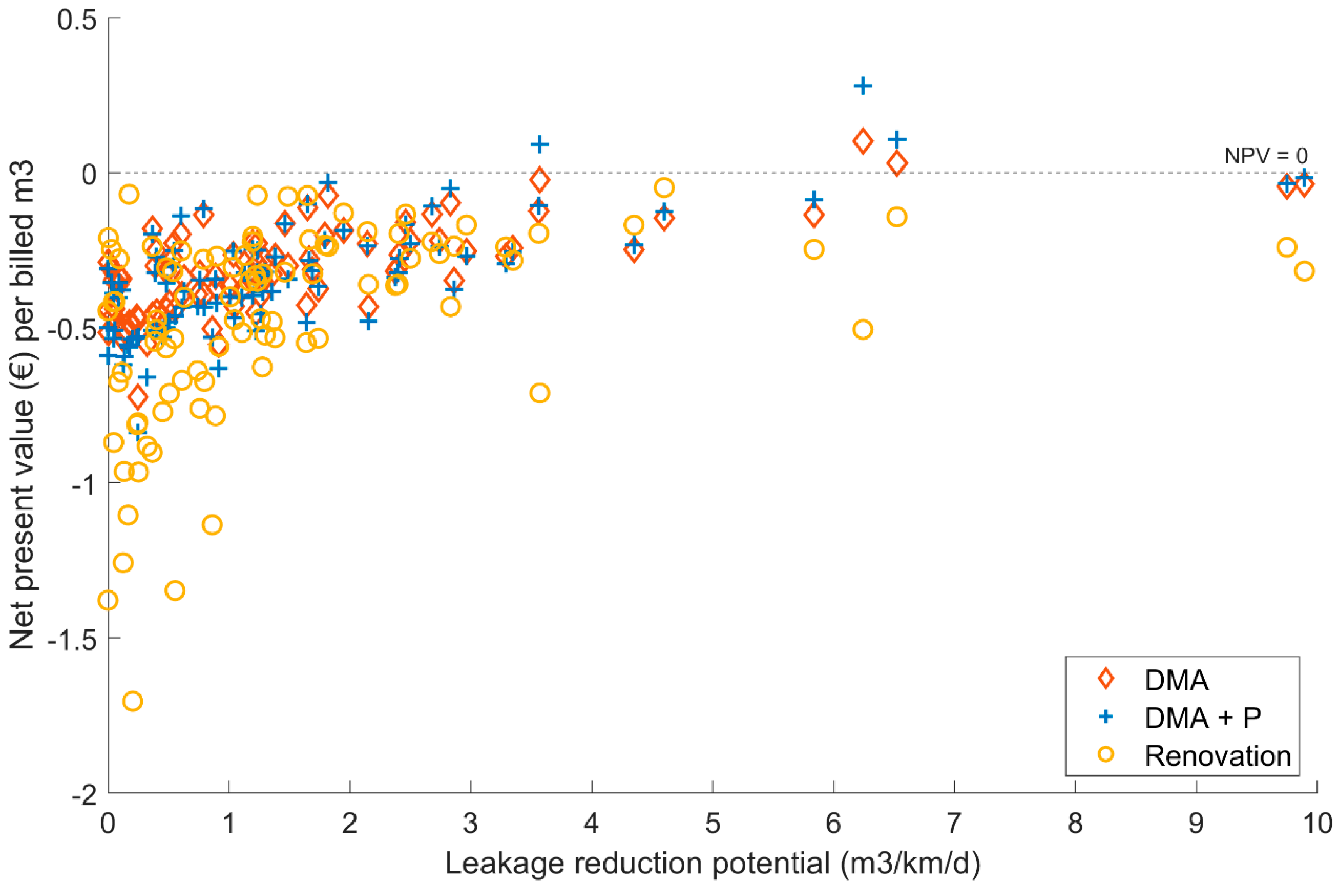
We calculated the net present values (NPV) for three leakage reduction measures: (1) district metering (DMA), (2) district metering with pressure reduction (DMA + P), and (3) renovations (Figure 3). Only three of the 92 utilities had at least one positive NPV; both were for DMA and DMA + P. Renovations were not a cost–beneficial leakage reduction measure for any of the utilities. Overall, the NPVs are small (negative) compared to the median marginal cost of water (0.11 euros/m3) of our utilities. The median NPV was −0.32 euros/billed m3 for DMA, −0.34 euros/billed m3 for DMA + P, and −0.36 euros/billed m3 for renovations.
District metering was the most cost-effective measure for a majority (55%) of the utilities, even though most NPVs were still negative. Renovations were the best measure for 29% of the utilities, and district metering with pressure reduction was the best measure for 15% of the utilities. In the case of renovations, the main benefit came almost always from the decrease in pipe failures, while the benefit of reducing the water loss was smaller.
3.3. The Economic Level of Leakage (ELL)
We calculated the economic levels of leakage (ELL), which is the point where the costs and benefits of leakage management add up to zero. Due to the mostly negative cost–benefit values, most utilities had a higher ELL than the current leakage level. The median of the best ELLs of each utility expressed as m3/km/day was 4.6, or 39% as leakage percentage, while the current median leakage levels are 1.6 m3/km/day and 17% in terms of percentage of water input. Naturally, it is not guaranteed that the systems would actually work with such high theoretical leakage levels.
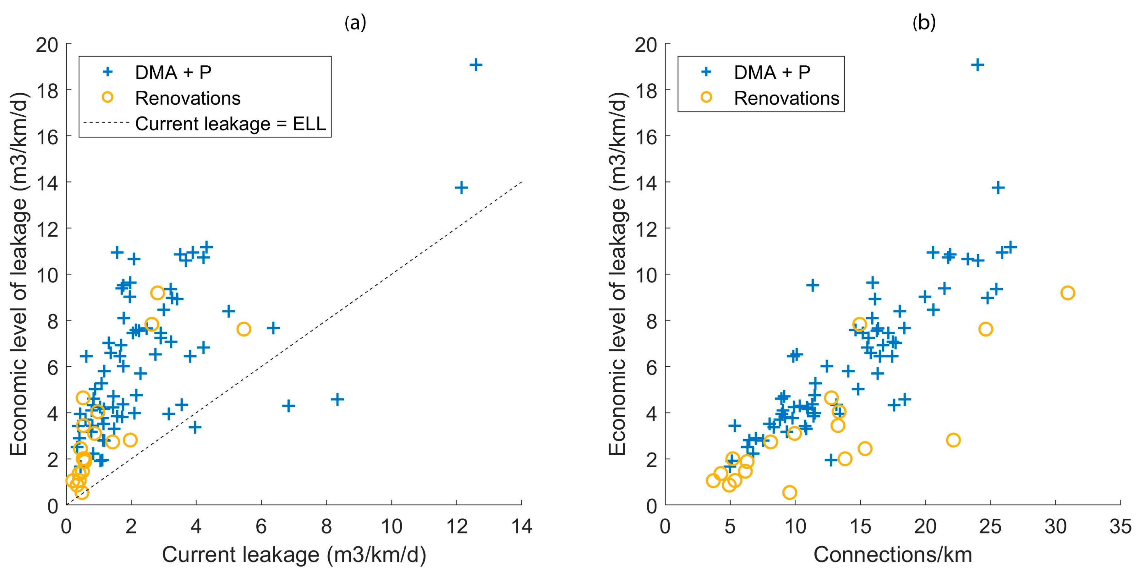
Figure 4 shows the ELL values of the best performing measure of each utility against (a) the current leakage level and (b) the connection density. Even though district metering (DMA) alone was the most beneficial measure for a majority of the utilities at the current leakage levels, there is a point at which the net present value of district metering combined with pressure management (DMA + P) surpasses the DMA. At the economic level of leakage, the first investment to make includes pressure management for a majority of the utilities.
The limitation of this approach is that the selected leakage reduction measures require large, expensive investments which result in relatively high ELL values. In reality, labor-intensive active leakage detection is part of the equation and would most likely lower the ELL in terms of the ILIs.
3.4. Uncertainty and Sensitivity Analysis
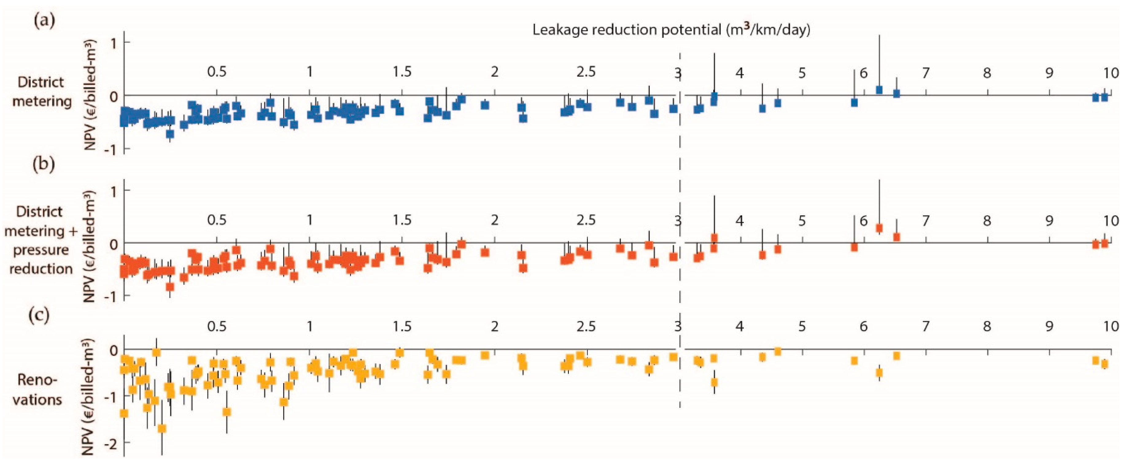
The uncertainty of the final net present values of the leakage reduction measures was estimated using Monte Carlo simulations. Figure 5 shows the median values of the results along with the 10th and 90th percentiles for (a) district metering, (b) district metering with pressure reduction, and (c) renovations. For some utilities, the variation is considerable, but the overall conclusion that the measures are not cost-effective for most of the utilities does not change.
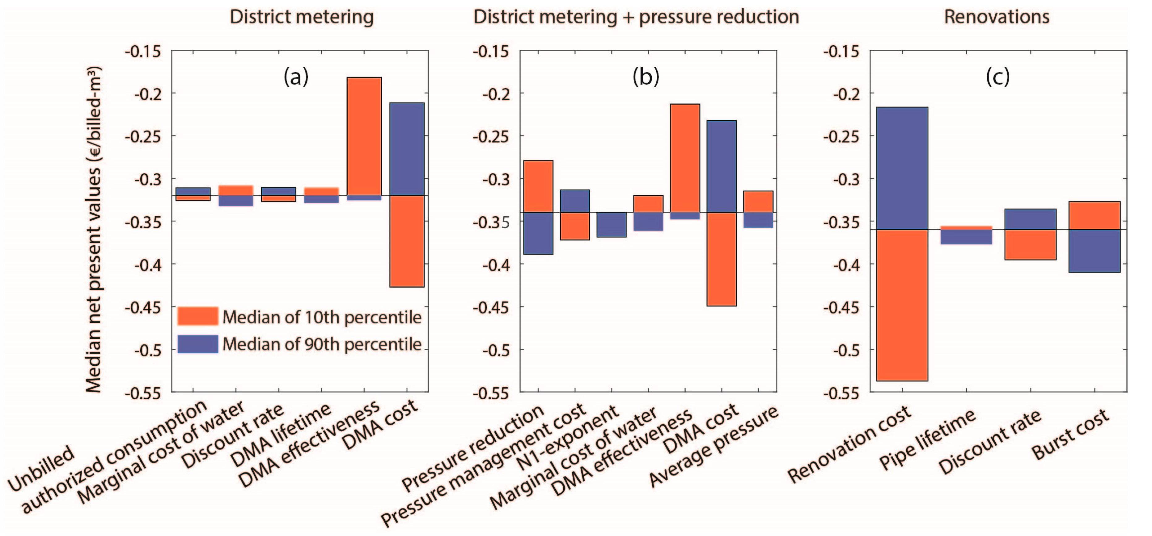
The effect of individual input variables on the output was similarly tested by one-at-a-time Monte Carlo simulations. Figure 6 shows the median value of the 10th and 90th percentiles of each utility’s simulated results. The bars start from the median value of the baseline results. More parameters were tested, but only the most influential are shown in the figure. The investment costs of district metering stations as well as the renovation cost had the highest influences on the final net present values.
4. Discussion
4.1. Context-Specific Findings: Mostly Low Water Loss Levels in Finland
According to our results, the majority of Finnish utilities have low or moderate levels of water loss. Moreover, only three utilities had positive returns on leakage reduction investments based on the direct costs and benefits gained by the utilities. As a result, the economic levels of leakage (ELL) were mostly higher than the current leakage levels. The range of the ELLs expressed as leakage per network length per day (m3/km/day) was wide (0.5–19), which means that no threshold value for the cost-benefit of leakage reduction measures could be identified in terms of this leakage indicator. In terms of leakage percentage, the ELLs were 10%–59%. The values are high but not necessarily unfeasible, since the current leakage level is at highest 49%. The highest ELL percentages resulted for utilities that have lower connection densities and lower burst rates.
One reason for the low net present values (NPVs) is the relatively low marginal cost of water. The median cost of water with the Finnish data was 0.11 euros/m3, which is in the lower end compared to European case studies with costs between 0.09 and 0.51 euros/m3 [40].
4.2. Leakage Reduction Methods
Based on our data, reducing water loss through investment-based measures is not cost-efficient for most water utilities in Finland. However, we did not consider the benefit that comes from the avoidance of increasing raw water source and treatment capacity or of improving the network reliability, other than the direct costs saved through decreasing pipe failures. In comparison, between measures, district metering was clearly the best method, although pressure management increased the benefits for a number of utilities. The uncertainty analysis showed that the conclusions are quite robust.
In other Nordic countries, one case study showed district metering or increased labor-intensive leakage detection efforts to be the most economical methods for leakage reduction [8]. Another case study indicated that renovations were not cost-effective for water loss reduction [7], similarly to our study. In line with our results is also the Italian case study by Creaco and Walski [41], which concluded that pressure control is not cost-effective if the water loss level and the marginal cost of water are low.
Our results were most sensitive to the variables district metering cost and renovation cost followed by DMA effectiveness, burst cost, and pressure reduction potential. The cost of district metering varies depending on the number of metering stations, among other things, and is quite case-specific. Along with pressure management cost, it should be evaluated individually for cost–benefit calculations. With the assumptions of our study, the investments would still remain uneconomic for most utilities. However, the utilities get other value from district metering, such as increased system control possibilities, which were not taken into account.
Data on average renovation cost are more suitable to generalization. We had data from eight utilities, which represented both larger cities as well as smaller towns, giving a good overview of the renovation costs in different surroundings. During the work for this article, the variable ‘number of connection’ was added to the national water utility database (VEETI). This increased the reliability of the results considerably, as earlier the connection density was identified as one of the most sensitive variables.
Some uncertainties remain in our analysis. Around 14% of the utilities had clearly made some errors in filling in the data in the VEETI database, and it is possible that we could not identify all such cases. One major gap in the analysis is that we did not account for the effect of possible future demand growth. Future demand growth can necessitate increasing treatment capacity and augmenting water sources. Since we did not conduct individual interviews with each utility, we had no information on whether they are close to their capacity limits.
4.3. Leakage Indicators and Policies
The majority of the utilities, concentrating on the small and medium-sized utilities, got the theoretically impossible ILI value of less than one. This means that the estimated minimum leakage level (UARL) is higher than the reported leakage level. In terms of leakage per water input to the network, the UARL was over 30% for 14 utilities and even over 50% for one utility. This shows how low some of the connection densities are in Finland. Earlier, it was instructed that the ILI formula is applicable only to connection densities above 20 connections/km [42], but this restriction was later removed, while the median connection density of the small utilities in our data is 11 connections/km.
According to [42], the empirical estimates in the UARL formula are derived mostly from tests in district metered areas in England and Wales during the late 1990s. For example, the UARL of the main pipes is a combination of background leakage and leakage from reported and unreported breaks. All of these components are affected by network material and age. Further studies are needed to clarify whether the empirical parameters of the ILI formula are applicable to utilities with low connection densities and relatively young pipes, as is the case in Finland.
It is clear that percentual leakage targets are not very suitable, even when used internally at utilities, because the leakage percentage is a function of water use. Our results suggest that the ILI, even though theoretically more appropriate, is also not a suitable indicator for setting leakage targets in Finland. Instead, in the absence of a suitable indicator, the utilities could be obligated to monitor leakage levels and formulate leakage management plans in the long term.
5. Conclusions
The analysis showed that water loss management is often not directly cost-beneficial to utilities operating with moderate leakage levels. Calculating the economic levels of leakage did not yield leakage target levels that could be generalized within a country. This shows that the target levels should be determined individually. Moreover, neither the leakage percentage nor the Infrastructure Leakage Index (ILI) were suitable for leakage target setting. The costs of investing in district metering or renovations were the most influential factors in the sensitivity analysis, followed by district metering effectiveness, burst cost, and pressure reduction potential. However, the estimated values were sufficiently accurate for reaching our conclusions.
Author Contributions
The authors have contributed to the article accordingly: conceptualization, S.A.; methodology, S.A.; formal analysis, S.A.; investigation, S.A.; data curation, S.A.; writing—original draft preparation, S.A.; writing—review and editing, S.A. and R.V.; visualization, S.A.; supervision, R.V.; project administration, S.A. and R.V.; funding acquisition, R.V. and S.A. All authors have read and agreed to the published version of the manuscript.
Funding
This research was financially supported by the Finnish Ministry of Agriculture and Forestry (grant number 2267/311/2014) and Maa-ja vesitekniikan tuki ry.
Conflicts of Interest
The authors declare no conflict of interest. The funders had no role in the design of the study; in the collection, analyses, or interpretation of data; in the writing of the manuscript, or in the decision to publish the results.
References
- Liemberger, R.; Wyatt, A. Quantifying the global non-revenue water problem. Water Supply 2019, 19, 831–837. [Google Scholar] [CrossRef]
- Puust, R.; Kapelan, Z.; Savic, D.A.; Koppel, T. A review of methods for leakage management in pipe networks. Urban Water J. 2010, 7, 25–45. [Google Scholar] [CrossRef]
- Hamilton, S.; Charalambous, B. Leak Detection: Technology and Implementation; IWA Publishing: London, UK, 2013; ISBN 978-1-78040-471-4. [Google Scholar]
- Gomes, R.; Sá Marques, A.; Sousa, J. Identification of the optimal entry points at District Metered Areas and implementation of pressure management. Urban Water J. 2012, 9, 365–384. [Google Scholar] [CrossRef]
- Vicente, D.J.; Garrote, L.; Sánchez, R.; Santillán, D. Pressure Management in Water Distribution Systems: Current Status, Proposals, and Future Trends. J. Water Resour. Plan. Manag. 2016, 142, 04015061. [Google Scholar] [CrossRef]
- Environment Agency; Ofwat; Defra. Review of the Calculation of Sustainable Economic Level of Leakage and Its Integration with Water Resource Management Planning; Environment Agency: Bristol, UK, 2012.
- Venkatesh, G. Cost-benefit analysis—leakage reduction by rehabilitating old water pipelines: Case study of Oslo (Norway). Urban Water J. 2012, 9, 277–286. [Google Scholar] [CrossRef]
- Malm, A.; Moberg, F.; Rosén, L.; Pettersson, T.J.R. Cost-Benefit Analysis and Uncertainty Analysis of Water Loss Reduction Measures: Case Study of the Gothenburg Drinking Water Distribution System. Water Resour. Manag. 2015, 29, 5451–5468. [Google Scholar] [CrossRef]
- Martins, R.; Coelho, F.; Fortunato, A. Water losses and hydrographical regions influence on the cost structure of the Portuguese water industry. J. Product. Anal. 2012, 38, 81–94. [Google Scholar] [CrossRef] [Green Version]
- Ferro, G.; Mercadier, A.C. Technical efficiency in Chile’s water and sanitation providers. Util. Policy 2016, 43, 97–106. [Google Scholar] [CrossRef]
- Molinos-Senante, M.; Mocholí-Arce, M.; Sala-Garrido, R. Estimating the environmental and resource costs of leakage in water distribution systems: A shadow price approach. Sci. Total. Environ. 2016, 568, 180–188. [Google Scholar] [CrossRef]
- Islam, M.S.; Babel, M.S. Economic Analysis of Leakage in the Bangkok Water Distribution System. J. Water Resour. Plan. Manag. 2013, 139, 209–216. [Google Scholar] [CrossRef]
- Ross, S.A. Uses, Abuses, and Alternatives to the Net-Present-Value Rule. Financ. Manag. 1995, 24, 96–102. [Google Scholar] [CrossRef]
- Finland’s Environmental Administration. Vesihuoltolaitosten Raportteja [Several Data Files]. Available online: http://www.ymparisto.fi/fi-FI/Kartat_ja_tilastot/Vesihuoltoraportit/Vesihuoltolaitosten_raportit/ (accessed on 10 April 2018). (In Finnish)
- Energy Authority. Sähkön Hintatilastot. Available online: https://www.energiavirasto.fi/sahkon-hintatilastot (accessed on 10 March 2017). (In Finnish).
- Ojala, M. Kiinteistöjen Tonttivesijohtojen ja -Viemäreiden Saneeraus, KTVVS-Tutkimus 2001; VVY:n monistesarja 9: Helsinki, Finland, 2002. (In Finnish) [Google Scholar]
- Lapinlampi, T.; Raassina, S. Water Supply and Sewer Systems 1998—2000. Waterworks (In Finnish); The Finnish Environment 541: Helsinki, Finland, 2002. [Google Scholar]
- Ahopelto, L.; Veijalainen, N.; Guillaume, J.; Keskinen, M.; Marttunen, M.; Varis, O. Can There be Water Scarcity with Abundance of Water? Analyzing Water Stress during a Severe Drought in Finland. Sustainability 2019, 11, 1548. [Google Scholar] [CrossRef] [Green Version]
- Heino, O.; Takala, A.; Katko, T. Challenges to Finnish water and wastewater services in the next 20–30 years. E-WAter 2011, 1–20. [Google Scholar]
- Seppälä, O. IWA Yearbook 2013—Finland. Available online: http://www.vesiyhdistys.fi/english.html (accessed on 28 March 2017).
- Rajala, R.P.; Hukka, J.J. Asset life cycle management in Finnish water utilities. J. Water Resour. Prot. 2018, 10, 587–595. [Google Scholar] [CrossRef] [Green Version]
- Alegre, H.; Baptista, J.F.d.M.; Cabrera, E.; Cubillo, F.; Duarte, P.; Hirner, W.; Merkel, W.; Parena, R. Performance Indicators for Water Supply Services, 2nd ed.; IWA Publishing: London, UK, 2006; ISBN 978-1-78040-633-6. [Google Scholar]
- van Zyl, J.E.; Lambert, A.O.; Collins, R. Realistic Modeling of Leakage and Intrusion Flows through Leak Openings in Pipes. J. Hydraul. Eng. 2017, 143, 04017030. [Google Scholar] [CrossRef]
- Lambert, A. What do we know about pressure/leakage relationships in distribution systems? In Proceedings of the IWA Specialised Conference, System Approach to Leakage Control and Water Distribution Systems Management, Brno, Czech Republic, 16–18 May 2001. [Google Scholar]
- Lambert, A.O.; Fantozzi, M. Recent developments in pressure management. In Proceedings of the Water Loss 2010 Conference, Sao Paolo, Brazil, 6–9 June 2010. [Google Scholar]
- Tuhovcak, L.; Suchacek, T.; Rucka, J. The Dependence of Water Consumption on the Pressure Conditions and Sensitivity Analysis of the Input Parameters. Proceedings 2018, 2, 592. [Google Scholar] [CrossRef] [Green Version]
- Berninger, K.; Laakso, T.; Paatela, H.; Virta, S.; Rautiainen, J.; Virtanen, R.; Tynkkynen, O.; Piila, N.; Dubovik, M.; Vahala, R. Sustainable Water Services for the Future—Direction, Steering and Organisation; Prime Minister’s Office: Helsinki, Finland, 2018. (In Finnish)
- Järvenpään Vesi. Järvenpään Vesihuoltoverkostojen Saneerausohjelma. Available online: https://www.jarvenpaa.fi/jarvenpaa/attachments/text_editor/774.pdf (accessed on 10 March 2017). (In Finnish).
- Pöyry. Verkostosaneerausten Vaikuttavuuden Arviointi, Raportti 67090591.BBP. Available online: https://docplayer.fi/360892-Verkostosaneerausten-vaikuttavuuden-arviointi.html (accessed on 2 October 2019). (In Finnish).
- Pietarila, V. Evaluation of Renovation Debt in Water Supply Network in Oulu. Bachelor’s Thesis, Oulu University of Applied Sciences, Oulu, Finland, 2012. (In Finnish). [Google Scholar]
- Polvinen, H.-L. Vesiputkien Taloudellisesti Optimaalinen Saneerausajankohta. Master’s Thesis, University of Oulu, Oulu, Finland, 2015. (In Finnish). [Google Scholar]
- ELY Centre. Vesihuoltoverkoston Saneeraustarpeen Selvittäminen: Työkaluja Varojen Kohdentamiseen; Reports 10/2017; The Southeast Finland Centre for Economic Development, Transport and the Environment: Turku, Finland, 2017. (In Finnish) [Google Scholar]
- Pianosi, F.; Sarrazin, F.; Wagener, T. A Matlab toolbox for Global Sensitivity Analysis. Environ. Model. Softw. 2015, 70, 80–85. [Google Scholar] [CrossRef] [Green Version]
- Pianosi, F.; Beven, K.; Freer, J.; Hall, J.W.; Rougier, J.; Stephenson, D.B.; Wagener, T. Sensitivity analysis of environmental models: A systematic review with practical workflow. Environ. Model. Softw. 2016, 79, 214–232. [Google Scholar] [CrossRef]
- Lam, K.L.; Kenway, S.J.; Lant, P.A. City-scale analysis of water-related energy identifies more cost-effective solutions. Water Res. 2017, 109, 287–298. [Google Scholar] [CrossRef] [Green Version]
- Lemos, D.; Dias, A.C.; Gabarrell, X.; Arroja, L. Environmental assessment of an urban water system. J. Clean. Prod. 2013, 54, 157–165. [Google Scholar] [CrossRef]
- Pillot, J.; Catel, L.; Renaud, E.; Augeard, B.; Roux, P. Up to what point is loss reduction environmentally friendly? The LCA of loss reduction scenarios in drinking water networks. Water Res. 2016, 104, 231–241. [Google Scholar] [CrossRef] [PubMed]
- LNEC; ERSAR. Water and Waste Services Quality Assessment Guide. 2nd Generation of the Assessment System; Water and Waste Services Regulation Authority (ERSAR), National Laboratory for Civil Engineering (LNEC): Lissabon, Portugal, 2013; p. 71. [Google Scholar]
- Svenskt Vatten. Hållbarhetsindex för Kommunernas VA-Verksamhet, Beskrivning av Verktygets Syfte och Konstruktion inför Undersökningen 2017; Svenskt Vatten AB: Stockholm, Sweden, 2017; p. 34. (In Swedish) [Google Scholar]
- European Commission. Resource and Economic Efficiency of Water Distribution Networks in the EU; Final Report (ENV.D.1/SER/2010/0029); European Union: Brussels, Belgium, 2013. [Google Scholar]
- Creaco, E.; Walski, T. Economic Analysis of Pressure Control for Leakage and Pipe Burst Reduction. J. Water Resour. Plan. Manag. 2017, 143, 04017074. [Google Scholar] [CrossRef]
- Lambert, A. Ten Years’ Experience in Using the UARL Formula to Calculate Infrastructure Leakage Index. In Proceedings of the Water Loss 2009 Conference, Cape Town, South Africa, 26–30 April 2009. [Google Scholar]
Figure 1.
Steps of the analysis for calculating the net present value of three leakage reduction measures: (1) district metering areas, (2) district metering areas with pressure reduction, and (3) renovations.
Figure 1.
Steps of the analysis for calculating the net present value of three leakage reduction measures: (1) district metering areas, (2) district metering areas with pressure reduction, and (3) renovations.

Figure 2.
The current leakage level, the minimum leakage level according to the unavoidable annual real losses (UARL) formula, and the devised minimum leakage level in terms of leakage volume in m3/km of the Finnish utilities plotted against the density of people per kilometre of network.
Figure 2.
The current leakage level, the minimum leakage level according to the unavoidable annual real losses (UARL) formula, and the devised minimum leakage level in terms of leakage volume in m3/km of the Finnish utilities plotted against the density of people per kilometre of network.

Figure 3.
Net present values per volume of billed water (euros/m3) for the leakage reduction measures: (1) district metered areas (DMA), (2) district metered areas with pressure reduction (DMA + P), and (3) renovations plotted against the leakage reduction potential (m3/km/d).
Figure 3.
Net present values per volume of billed water (euros/m3) for the leakage reduction measures: (1) district metered areas (DMA), (2) district metered areas with pressure reduction (DMA + P), and (3) renovations plotted against the leakage reduction potential (m3/km/d).

Figure 4.
The economic level of leakage in terms of leakage per network length per day for each utility against (a) the current leakage level and (b) the connection density. The markers show which leakage reduction measure is the most cost-beneficial for each utility.
Figure 4.
The economic level of leakage in terms of leakage per network length per day for each utility against (a) the current leakage level and (b) the connection density. The markers show which leakage reduction measure is the most cost-beneficial for each utility.

Figure 5.
Net present values (euros) per total billed volume of water in m3 for: (a) District metering; (b) District metering with pressure reduction; and (c) Renovations in relation to the leakage reduction potential. The simulated 10th to 90th percentile values are indicated by the error bars. Note that the scale of the x-axes changes at 3 m3/km/day.

Figure 6.
Median net present values for baseline (horizontal line) and the median of the 90th percentile (blue bar) and 10th percentile (red bar) results for: (a) District metering; (b) District metering with pressure reduction; and (c) Renovations.
Figure 6.
Median net present values for baseline (horizontal line) and the median of the 90th percentile (blue bar) and 10th percentile (red bar) results for: (a) District metering; (b) District metering with pressure reduction; and (c) Renovations.


Table 1.
The estimated pipe failure rates (failures/100 km/year) for different material groups for ‘old’ and ‘new’ pipes, the ratio between the average failure rate and the failure rate of ‘old’ pipes, and the leakage rate of different material groups compared to the metal group.
Table 1.
The estimated pipe failure rates (failures/100 km/year) for different material groups for ‘old’ and ‘new’ pipes, the ratio between the average failure rate and the failure rate of ‘old’ pipes, and the leakage rate of different material groups compared to the metal group.
| Age Category | Pipe Failure Rate (Failures/100 km/year) | ||
|---|---|---|---|
| Metal | Plastic | Other/Unknown | |
| Old (≥50 or ≥40 years old) | 16 | 10 | 6 |
| New (≤15 years old) | 1 | 1 | 0 |
| Average of all ages | 9 | 1 | 3.3 |
| Ratio of old to average pipe failure rate | 1.8 | 7.1 | 1.8 |
| Leakage rate compared to metal pipes (based on the average pipe failure rates) | 1 | 0.15 | 0.36 |
Table 2.
The distributions of variables in the uncertainty analysis. DMA: district metered areas.
| Variable | Unit | Distribution | Estimated Mean (µ) | Standard Deviation (σ) | Uniform Dist. Bounds |
|---|---|---|---|---|---|
| The total length of service lines | m | normal | 22.5 | 5 | - |
| Unbilled authorized consumption | % of network input | uniform | 2 | - | [0.5, 3.5] |
| Average pressure | m | uniform | 50 | - | [35, 65] |
| Discount rate | % per year | normal | 3.5 | 0.8 | - |
| Marginal cost of water | euros/m3 | truncated normal | varies by utility (median 0.11) | 0.1 µ (min. value 0.04) | - |
| DMA effectiveness | % of the total leakage reduction potential | uniform | 30 | - | [20, 100] |
| DMA cost | euros/DMA area | normal | 48,000 | 10,000 | - |
| DMA lifetime | years | normal | 20 | 2 | - |
| N1 (leakage–pressure exponent) | - | uniform | varies by utility | - | [0.5, 1.5] |
| Average pressure reduction | m | uniform | 5 | [1, 10] | |
| Cost of pressure management | euros/station | normal | 9000 | 2000 | - |
| Burst repair cost | euros | truncated normal | 5500–14,500 (varies by utility size) | 0.25 µ (min. value 2000) | - |
| Renovation cost | euros/metre | truncated normal | 94–628 (varies by utility size) | 0.25 µ (min. value 50) | - |
| Pipe lifetime | years | normal | 70 | 15 | - |
Table 3.
Median, minimum and maximum values for key leakage level characteristics for the 92 Finnish water utilities grouped by size, and the share of utilities with leakage reduction potential in the size groups in 2015–2017.1 ILI: Infrastructure Leakage Index.
Table 3.
Median, minimum and maximum values for key leakage level characteristics for the 92 Finnish water utilities grouped by size, and the share of utilities with leakage reduction potential in the size groups in 2015–2017.1 ILI: Infrastructure Leakage Index.
| Utility Size (Sample Size) | Figure | Service Conn/km | No. of People/km | Leakage % 2 | Leakage m3/km/d | ILI |
|---|---|---|---|---|---|---|
| Small (n = 43), | ||||||
| 3000–10,000 pop., | Median | J | F | J | J | J |
| 900–3700 conn. | Min–Max | 4–21 | 7–67 | 4–49 | 0.2–7 | 0.2–4.4 |
| Medium (n = 39), | ||||||
| 10,000–60,000 pop., | Median | J | M | J | J | J |
| 2000–16,000 conn. | Min–Max | 5–31 | 17–198 | 6–28 | 0.4–5 | 0.3–2.2 |
| Large (n = 10), | ||||||
| 60,000–1200,000 pop., | Median | J | M | J | J | J |
| 11,000–73,000 conn. | Min–Max | 13–27 | 70–365 | 6–20 | 1–13 | 0.6–5.2 |
1 Data from 2015 were used for most utilities, but if unavailable, data from 2016 or 2017 were used. 2 Percentage of water input to the network.
© 2020 by the authors. Licensee MDPI, Basel, Switzerland. This article is an open access article distributed under the terms and conditions of the Creative Commons Attribution (CC BY) license (http://creativecommons.org/licenses/by/4.0/).
Share and Cite
MDPI and ACS Style
Ahopelto, S.; Vahala, R. Cost–Benefit Analysis of Leakage Reduction Methods in Water Supply Networks. Water 2020, 12, 195. https://doi.org/10.3390/w12010195
AMA Style
Ahopelto S, Vahala R. Cost–Benefit Analysis of Leakage Reduction Methods in Water Supply Networks. Water. 2020; 12(1):195. https://doi.org/10.3390/w12010195
Chicago/Turabian StyleAhopelto, Suvi, and Riku Vahala. 2020. "Cost–Benefit Analysis of Leakage Reduction Methods in Water Supply Networks" Water 12, no. 1: 195. https://doi.org/10.3390/w12010195
Note that from the first issue of 2016, this journal uses article numbers instead of page numbers. See further details here.