Spatial and Temporal Variability of Water Quality in the Bystrzyca River Basin, Poland


1
Department of Environmental Engineering and Geodesy, University of Life Sciences in Lublin, Leszczyńskiego 7, 20-069 Lublin, Poland
2
Department of Applied Mathematics and Computer Science, University of Life Sciences in Lublin, Głęboka 28, 20-612 Lublin, Poland
*
Author to whom correspondence should be addressed.
Water 2020, 12(1), 190; https://doi.org/10.3390/w12010190
Submission received: 1 December 2019
/
Revised: 31 December 2019
/
Accepted: 8 January 2020
/
Published: 9 January 2020
(This article belongs to the Section Water Quality and Contamination)
Abstract
:The aim of the study was to analyze the results of surface water quality tests carried out in the Bystrzyca river basin. The study was conducted over four years in four seasons. The following chemometric techniques were used for the purposes of statistical analyses: the principal component analysis with factor analysis (PCA/FA), the hierarchical cluster analysis (HCA), and the discriminant analysis (DA). The analyses allowed for determining the temporal variability in water quality between the seasons. The best water quality was recorded in summer and the worst in autumn. The analyses did not provide a clear assessment of the spatial variability of water quality in the river basin. Pollution from wastewater treatment plants and soil tillage had a similar effect on water quality. The tested samples were characterized by very high electrolytic conductivity, suspended solids and P-PO4 concentrations and the water quality did not meet the standards of good ecological status.
1. Introduction
In Poland, rivers are characterized by relatively low runoffs. Small water resources often overlap with eutrophication processes resulting from low dilution of pollutants. In the twentieth century, in Poland, often untreated municipal sewage and industrial wastewater was discharged directly into rivers. After Poland’s accession to the European Union (EU), the implementation of environmental monitoring programs commenced [1,2].
Due to their location, rivers carry pollutants to lakes and the sea, contributing to the eutrophication of these water bodies. Water from rivers, lakes, and groundwater is used for human consumption needs. Water resources play an important role in drinking water supply, crop irrigation, industrial production, hydropower generation, and fish farming [3,4,5,6]. The increase in water demand caused by the development of civilization has contributed to the reduction in the amount of water and the deterioration of its quality. Water quality is affected by both natural processes and anthropogenic factors. Natural processes include, but are not limited to, topography, geological structure, seasonal temperature and rainfall changes, and land use. Many studies confirm that natural processes have a significant impact on water quality [7,8,9,10]. However, anthropogenic factors are much more important for the deterioration of water quality [11,12]. The anthropogenic factors include: industrial pollution, domestic sewage, agricultural drainage, as well as agriculture and urbanization intensity. Pollutants go to water from point sources (industry, municipal) and area sources, which are identified with agricultural land [13,14,15]. Both natural and anthropogenic factors influence the amount of nutrients eluted from the basin [16,17]. Excessive content in surface waters can lead to eutrophication, oxygen deficiency, as well as the development of organisms posing a danger to human health [18,19]. Studies on the spatial variability of water quality have shown that the presence of nutrients in aquatic ecosystems is highly dependent on land use, soil properties, agriculture intensity, and the discharge of treated wastewater [20,21,22,23,24,25].
There is a need to assess surface water quality for proper water resource management. In order to protect water against pollution, it has become necessary to develop a water quality monitoring program. Long-term and regular research is a great source of information for water resource managers. The most commonly used methods for processing and analyzing datasets are multivariate statistics [26,27,28,29,30,31,32]. In addition, on their basis, it is possible to determine the variability between seasons, spatial variability of river water quality, and identify the potential sources of water pollution [4,33,34,35,36,37,38]. The following chemometric techniques were used for multivariate analysis of environmental datasets: the principal component analysis (PCA), the cluster analysis (CA), the discriminant analysis (DA), and the factor analysis (FA). Many studies also confirm the use of these techniques in order to identify the potential sources of water pollution. Chemometric techniques to assess the results of water quality testing have been used in many countries, e.g., India [33,34], Vietnam [35], Morocco [39], China [40,41], Hong Kong [42], Iraq [43], and Pakistan [44,45]. Such analyses were also carried out in Poland. PCA, CA, FA, and DA were used to analyze spatial and temporal changes in surface water quality in the Mała Wełna river basin [46]. Multivariate analyses, such as the principal component analysis with factor analysis (PCA/FA) and the hierarchical cluster analysis (HCA), were used in order to examine the effect of urbanization in the Łyna river basin on the water quality parameters [47]. On the example of Gdańsk, the cluster analysis (CA) and the analysis of variance (ANOVA) were used to analyze the temporal and spatial variability of drinking water quality. The sources of pollution in the Goczałkowice, Kowalskie, and Chechło reservoirs were also identified using multivariate statistical techniques [48,49,50].
Studies conducted so far in order to identify sources of water pollution indicate that water quality deteriorates mainly due to anthropogenic factors [51,52,53,54,55]. In the Bystrzyca river basin, surface water pollution results from agricultural activity, including animal husbandry, crop irrigation, and water erosion. This also overlaps with industrial activities, including the processing of sugar beets, fruits and vegetables, and the production of parts for cars and aircrafts. Due to the poor water quality in the Bystrzyca river basin, the environment monitoring program covering surface and underground waters has been carried out for 20 years (Regional Inspectorate for Environmental Protection). Regular monitoring and assessment of the water quality is necessary for the proper management of water resources in order to improve the status of the environment.
The aim of the study was to analyze the temporal and spatial variability of surface water quality in the Bystrzyca river basin. The dataset was collected over four years (2011–2014) in four seasons at 10 measuring stations (a total of 160 samples). To achieve this goal, chemometric techniques (HCA, PCA/FA, DA) were used, which allowed for: determining similarities and differences between the measuring stations, determining temporary changes in the water quality, and determining the potential sources of pollution affecting the water quality.
2. Material and Methods
2.1. Study Area
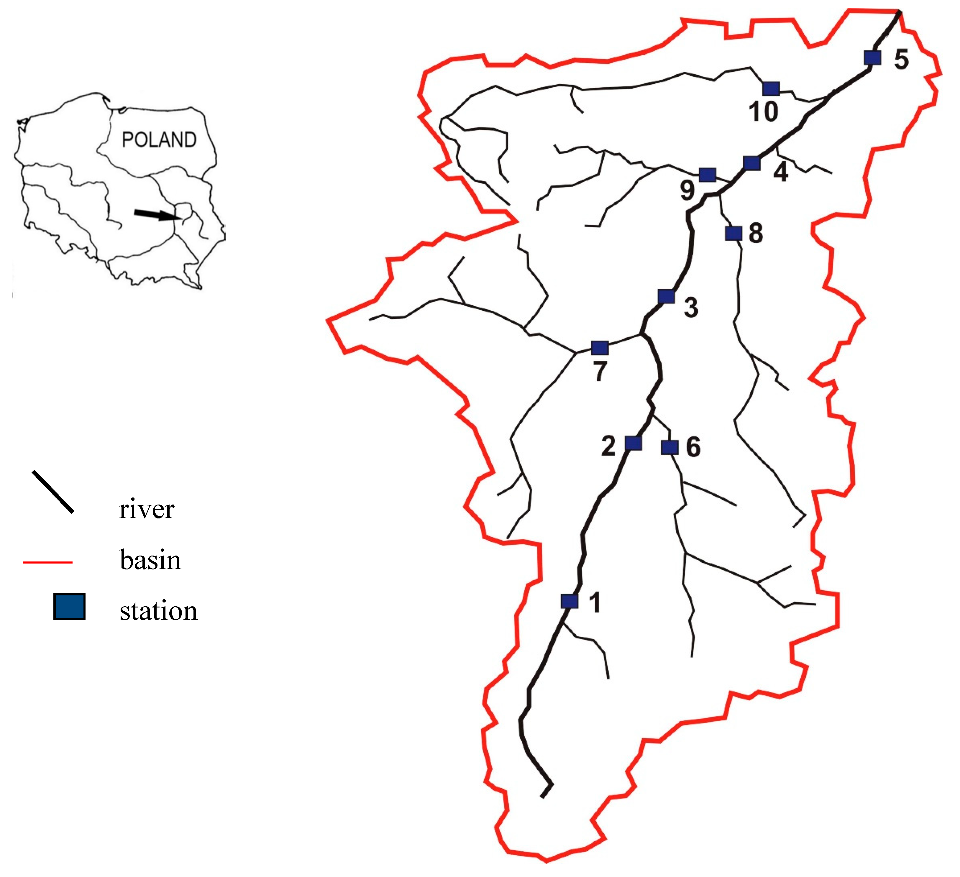
The Bystrzyca river basin, in terms of the physical and geographical location in Poland, is located in the macroregion of the Lublin Upland and in the mesoregions of the Świdnik Plateau and the Giełczew Plateau. According to the coding system for hydrographic units, the Bystrzyca river basin has the code 246 [56]. Typologically, Bystrzyca has been classified as a medium-sized river. Its ecological functioning is classified into various abiotic types: headwater section and all tributaries up to 6, middle section up to 9, and estuary section up to 15 [57]. The Bystrzyca River has its springs in Sulów at an altitude of 232 m above sea level, and the outlet near Spiczyn at an altitude of 152 m above sea level. The total area of the Bystrzyca basin is 1320 km2, and the part to the Sobianowice section, where hydrometric measurements were taken, covers 1260 km2. The river is 81.9 km long and is fed by five tributaries. The following tributaries have an outlet into the Bystrzyca River: Kosarzewka at 47 km, Kreżniczanka at 40 km, Czerniejówka at 26 km, Czechówka at 25 km, and Ciemięga at 12 km (from the outlet of the Bystrzyca river). From kilometer 18 to 38, the Bystrzyca River flows through the city of Lublin [51,52]. For this reason, the causes of eutrophication of surface water can be: intensive suburbanization, industrial activity, recreation, and agriculture. Suburbanization occurs in a ring-like system around the city of Lublin. Industry is mainly based in the eastern districts of the city. Recreational areas are concentrated in the southern part of the city, around the Zemborzyce reservoir. Agricultural areas are located downstream and upstream of the river. In 2014, five municipal sewage treatment plants and five industrial wastewater plants operated in the study area. In its catchment basin, there is the Zemborzyce reservoir with an area of 280 ha and three fishpond complexes with a total area of 70 ha. The basin includes agricultural land (78%): arable land constitutes 71%, grassland 4%, and orchards account for 3%. The land use structure of the basin is complemented by forestland (10%), urban areas (11%), and wasteland (1%). The soil cover consists mainly of Podzisols occurring in the top parts of the upland and on slopes, as well as Cambisols in the lowland parts [53,54,55]. In the years 2011–2014, the average annual air temperature was 9 °C, and the precipitation level was 570 mm. In the summer half-year, the precipitation was 370 mm, while in the winter half-year it was 200 mm. The average water runoff on the Sobianowice section was 4.1 m3 s−1, which was lower than the multi-year average.
2.2. Sample Collection
Surface water samples were collected for physical and chemical analyses over four years, 2011–2014, in four seasons (winter, spring, summer, autumn). A single 1 L sample was taken at each time at the depth of half of the water level in the river. The tests were carried out on five measuring sections along the Bystrzyca River and five on its tributaries (Table 1, Figure 1). Direct measurements with a Multi 340i multi-parameter meter (WTW, Weilheim, Germany) included: pH, dissolved oxygen (DO), and the electrolytic conductivity (EC) of water. Using the sampler, water samples were collected into PE bottles for laboratory testing. Physical and chemical analyses were carried out using a PC spectrophotometer (AQUALYTIC, Langen, Germany) and verified the following parameters: total phosphorus (P), phosphates (P-PO4), total nitrogen (N), and ammonium nitrogen (N-NH4), and by means of a LF300 photometer (SLANDI, Michałowice, Poland): sulphates (SO4) chloride (Cl), nitrate nitrogen (N-NO3), and Kjeldahl nitrogen (KN). Biochemical oxygen demand (BOD) was determined by the Winkler method, chemical oxygen demand (COD) by the bichromate method, suspended solids (SS) by the gravimetric method, and total organic carbon (TOC) using a TOC1200 analyzer (Trace Elemental Instruments, Delft, Netherlands).
Hydrometric measurements were also carried out at each measuring station, which included the measurement of water flow rate and cross-section parameters (river depth and width). This was done using a HEGA-1 hydrometric meter (Biomix, Poland) and a Leica Nova MS 50 total station (Leica, Switzerland).
2.3. Statistical Analysis
The assessment of the physical and chemical composition of the water in the Bystrzyca catchment basin was based on a set of data consisting of 15 water quality parameters. The study was carried out at ten measuring stations during the years 2011–2014 in four seasons (winter, spring, summer, autumn). Prior to the statistical analysis, the data was collated. Then, using the W test (Shapiro–Wilk), the compliance of the distribution of the physical and chemical parameters of water with normal distribution was checked. Environmental data was transformed and standardized to meet the normality assumption. In the case of chloride and sulphate concentrations, their distribution after transformation differed significantly from normal; therefore, these parameters were not included in chemometric analyses. In order to characterize the temporal and spatial variability of the remaining 13 water quality parameters, the multivariate analysis methods of classification and ordination were used. The hierarchical cluster analyses (HCA) were developed based on the monitoring stations’ measurements using the Ward’s minimum variance classification algorithm with Euclidean distance as a similarity measure. The principal component analysis with factor analysis (PCA/FA) was used to determine the relationships between water quality parameters at the measuring stations and individual test dates. Finally, the discriminant analysis (DA) was carried out, using the season as a discriminating variable. DA was applied to raw data, whereas CA and PCA were applied to standardized data to avoid misclassification arising from different parameter units.
3. Results and Discussion
3.1. Characteristics of Water Quality in the Bystrzyca River Basin
During the study period, the surface water in the Bystrzyca river basin showed an alkaline reaction ranging from 7.5 to 8.25. Nitrate nitrogen concentrations were low and ranged from 0.7 to 3.5 mg/L, ammonium nitrogen from 0.02 to 0.34 mg/L, and Kjeldahl nitrogen from 0.7 to 1.88 mg/L, while total nitrogen concentrations ranged from 1.5 to 5.2 mg/L. Low biochemical oxygen demand (BOD) was observed from 1.4 to 4.5 mg/L. Chemical oxygen demand (COD) ranged from 8.0 to 28.0 mg/L, and the concentrations of total organic carbon (TOC) ranged from 1.1 to 7.4 mg/L. Therefore, high DO concentrations above 7.6 mg/L could be observed. All the test samples were characterized by a very high content of suspended solids (SS), which ranged from 261 to 522 mg/L and the associated high electrolytic conductivity (EC) ranged from 393 to 802 μS/cm. In addition, high phosphorus concentrations ranging from 0.10 to 0.37 mg/L and very high phosphate concentrations (P-PO4) ranging from 0.05 to 0.24 mg/L were found in the test samples. The statistical parameters of water quality indicators for the testing seasons are presented in Table 2.
Based on the concentration of nitrogen, ammonium nitrogen, pH, DO, COD, and TOC, the water quality corresponded to a very good ecological status (class I). Based on the concentrations of total phosphorus, Kjeldahl nitrogen, nitrate nitrogen, and BOD, the water quality corresponded to good ecological status (class II). The standards of good ecological status are met for these oxygen and nutrient indicators. Achieving this goal was associated with the implementation of a program to protect the aquatic environment against degradation in the EU [2,51]. The test samples were characterized by very high EC, SS, and P-PO4 concentrations and the water quality did not meet the standards of good ecological status. Very high EC and SS concentrations are associated with the ionic composition of water and the runoff of soil and mineral salts from the slopes. Very high levels of orthophosphates are associated with the use of detergents and waste storage.
The analyzed surface waters had the best quality in the summer season, and the worst in the autumn season. The analysis of variance revealed fluctuations between the seasons in the study period in dissolved oxygen concentrations, biochemical oxygen demand, chemical oxygen demand, phosphates, electrolytic conductivity, and total phosphorus (statistically significant differences at the level α = 0.05). However, no differences in water quality parameters were found between the measuring stations.
3.2. Assessment of the Temporal and Spatial Variability
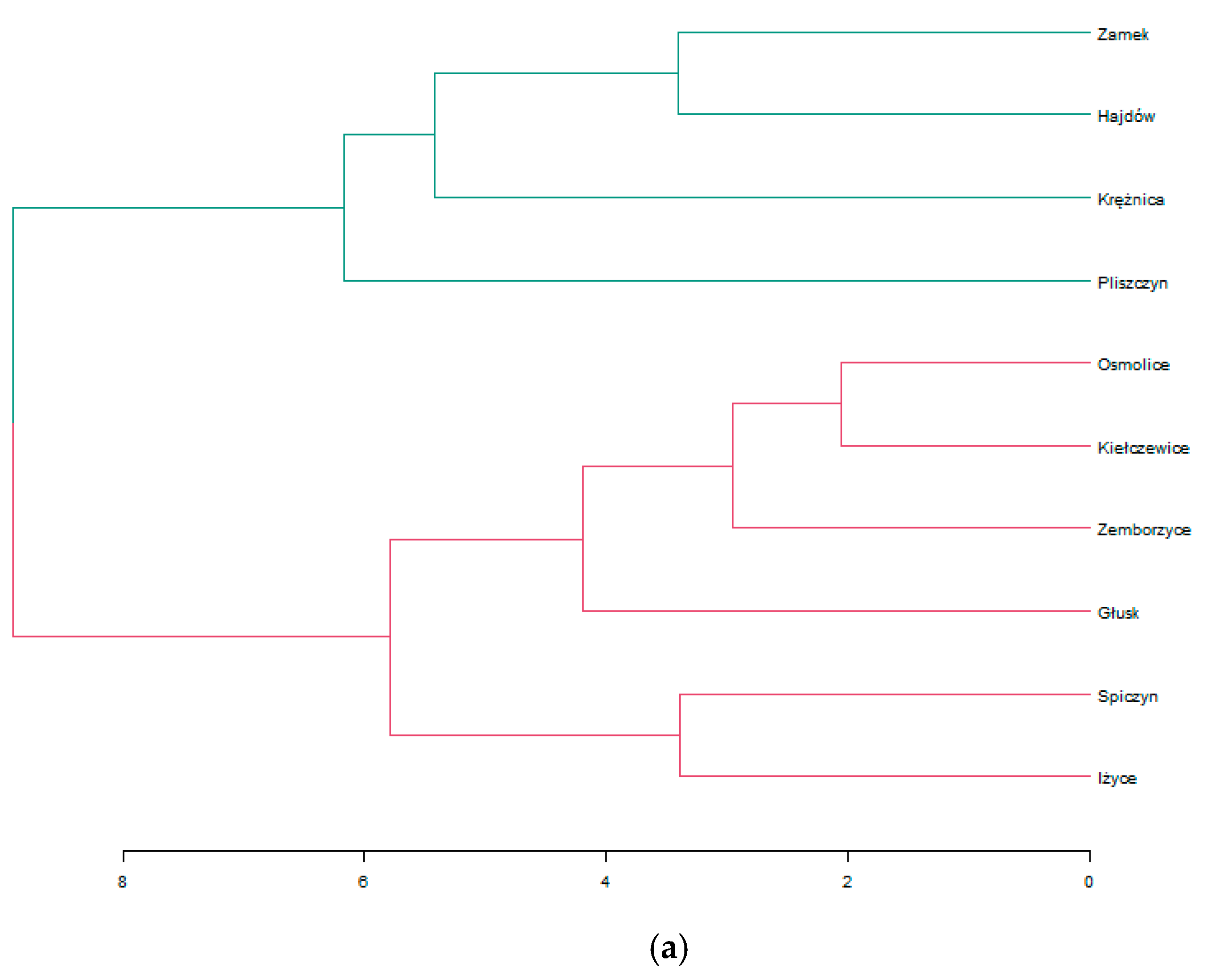
A hierarchical agglomerative cluster analysis was conducted to identify the temporal and spatial variability of water quality parameters at the monitored stations. Ward’s algorithm of minimum variance was used for clustering and the Euclidean distance was applied as a measure of similarity. The obtained results of classification are presented graphically as dendrograms (Figure 2a,b). The measuring sections were grouped into two statistically significant clusters (Dlink/Dmax) × 100 < 60. The first cluster consisted of the stations Pliszczyn, Krężnica, Zamek, and Hajdów (moderate pollution level). The stations Pliszczyn (10) and Krężnica (7) are located in eroded agricultural land, while the stations Zamek (9) and Hajdów (4) are located in an urban area. It follows that both intensive agriculture and urbanization contribute to water pollution. The second cluster includes the stations Kiełczewice (1), Osmolice (2), Zemborzyce (3), Spiczyn (5), Iżyce (6), and Głusk (8), with low water pollution (low pollution level). The investigated basin has a high capacity to retain dissolved chemical compounds. Therefore, the water quality parameters on the outlet stretch Spiczyn (5) have low values. In addition, despite the discharge of sewage from an industrial treatment plant, the Osmolice station was classified in the second group (low pollution level). It is similar in the case of the Hajdów station (moderate pollution level). This is where domestic sewage from the sewage treatment plant for the Lublin urban area (380,000 residents) is discharged. The cluster analysis detected no point source pollution in the form of industrial and domestic sewage discharges. This results from very good management of water resources and the use of the best available technology for wastewater treatment. In addition, point pollution is superimposed on area pollution from surface runoff. Stations located both in agricultural and urbanized areas were classified into one cluster. This indicates a comparable level of area and point pollution.
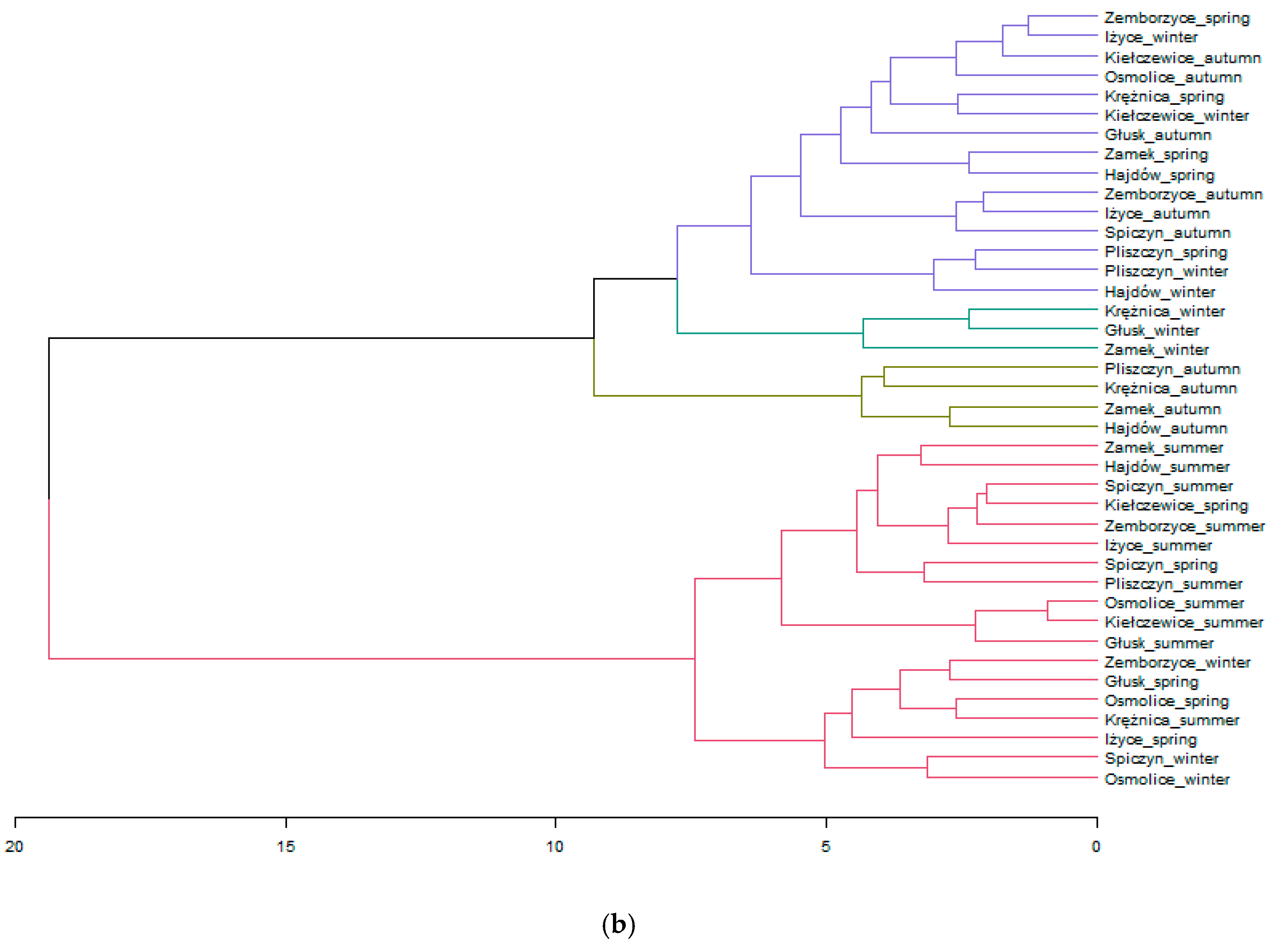
The CA was repeated taking into account both the stations and the date of sampling (Figure 2b). Four clusters were obtained and their analysis indicates that the date of sampling may be a factor determining that they should be included in a particular group. In particular, it can be seen that the samples taken in the summer season formed the first cluster (marked in pink). The second cluster comprised four samples from the autumn season (marked in olive green), while the third one comprised three samples from the winter season (marked in blue). The fourth cluster (marked in steel blue) includes the remaining samples from three different seasons. Samples taken during the summer and partly in the spring season show the lowest levels of pollution. This may be a result of highly diluted impurities and the uptake of nutrients by plants.
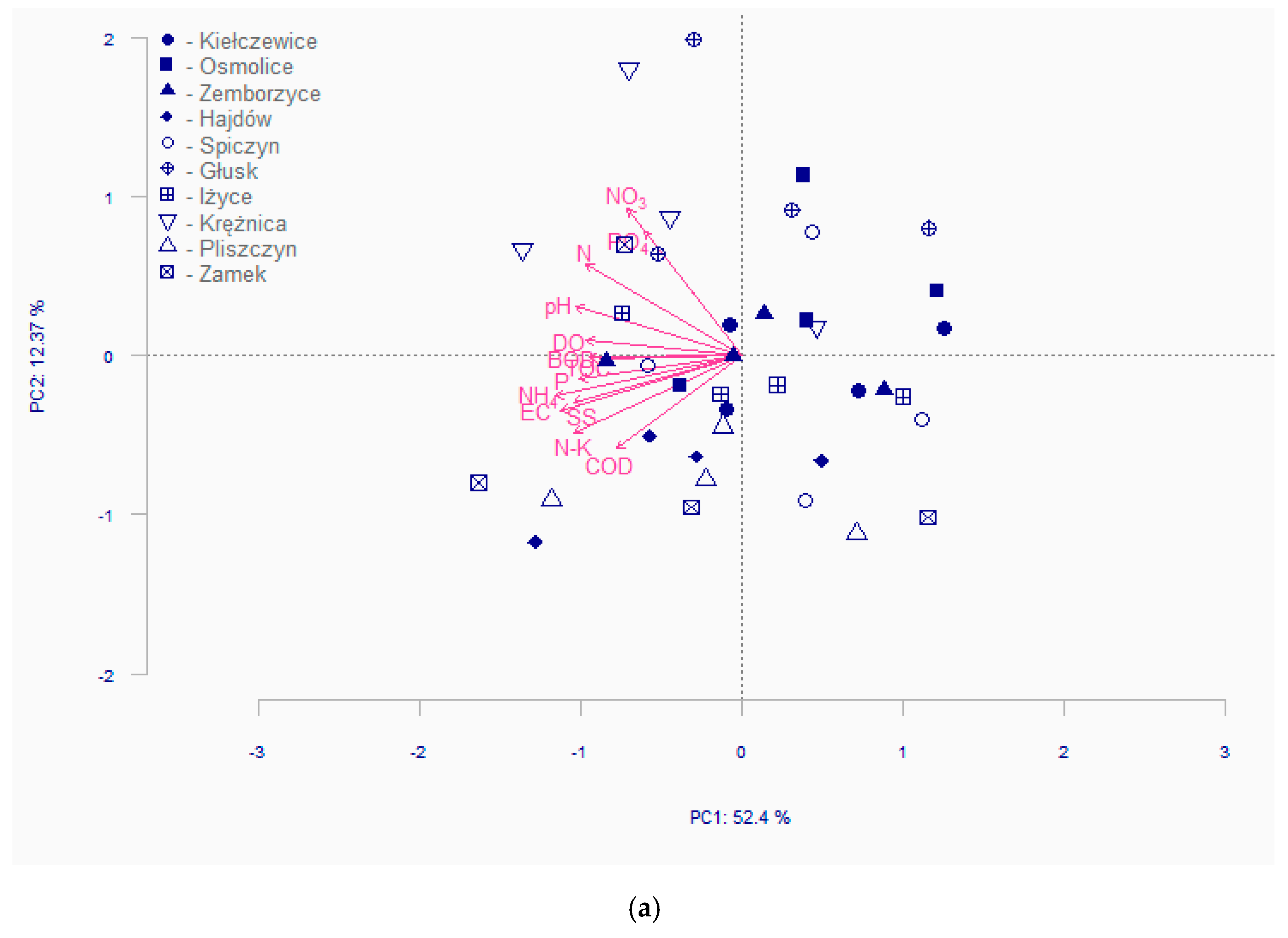
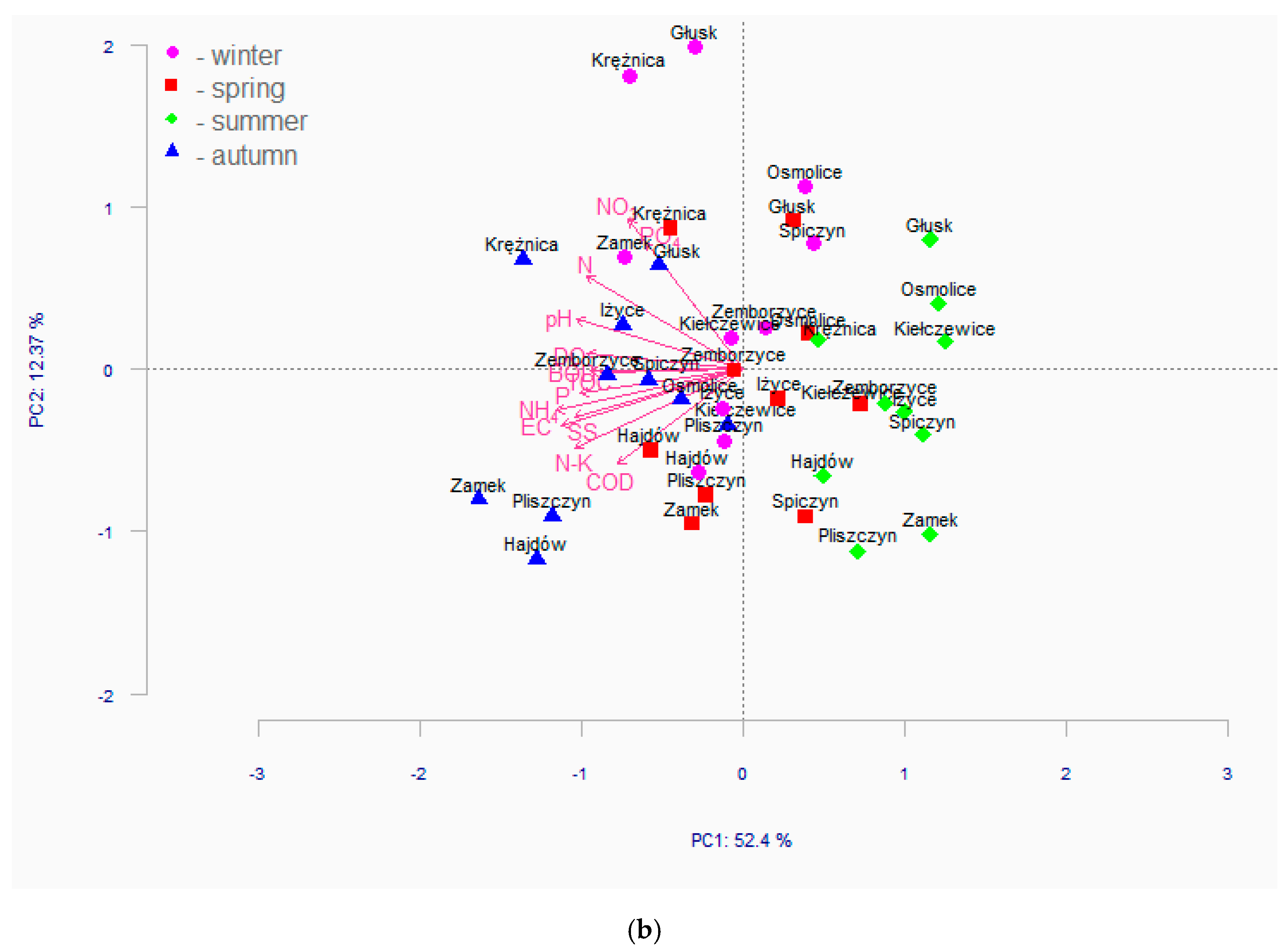
The next stage of the statistical analysis was the principal component analysis (PCA). Significant PCA axes were selected with the Kaiser–Gutman criterion [59]. The first three components (PC1, PC2, PC3) had eigenvalues greater than 1 (Table 3), which allowed 74.14% of the total variation to be explained. Assuming the assessment of the relationship between factor loadings for water quality parameters and individual components according to Reference [9], the following conclusions can be formulated. The factor analysis reduced the set of 13 parameters initially used to characterize water quality to three VF (Variations Factor) variations necessary for the identification of the river pollution sources. If the factor loadings between water quality parameters and VF coefficients are 0.75–1.00, the values are strongly correlated, while at 0.50–0.75, they are moderately correlated. The first factor, VF1 (corresponds to 68% of total variance), was strongly correlated with NK, N-NH4, EC, SS, pH, and P concentrations. The next two factors with a cumulative variance of 28% were, on average, correlated with the concentration of N-NO3 and P-PO4 (VF2), with organic carbon TOC (VF3). A negative factor correlation with the concentrations of nitrogen and phosphorus compounds suggests an impact of organic pollutants. These pollutants can be associated with intensive land use (fertilizers and pesticides) as well as industrial production (waste and sludge). Nitrogen and phosphorus compounds contribute to the eutrophication of water and the deterioration of the quality of aquatic ecosystems [60,61,62]. The negative correlation of the VF1 factor with pH level indicates that when the parameter has low values, carbon and calcium can be released from carbonate rocks. High concentrations of calcium carbonate occur in arable fields due to intensive soil erosion. A graphical representation of the PCA analysis for the first two components is shown in the graphs in Figure 3.
The principal component analysis did not provide an unambiguous assessment of the spatial variability of water composition in the catchment basin and its quality. Based on the PCA analysis, insignificant differences were identified in the physical and chemical parameters of the water analyzed on the sections Pliszczyn and Hajdów (Figure 3a), which is clearly influenced by both point sources of pollution (municipal sewage treatment plant) and area sources (soil erosion). No significant differentiation was found between the remaining points (the stations are mixed together).
However, the PCA analysis allowed significant differences in water quality to be determined between the testing seasons. With datasets for different periods, the PCA can also be used to investigate the temporal variations in water quality and find out the most important pollution sources for each period. By considering the deadline for sampling, the PCA can also be used to investigate the temporal variations in the water quality (Figure 3b). It can be seen that the first principal component is strongly correlated with the seasons. In particular, we can observe the clusters of samples in the summer and autumn seasons. The samples in the autumn season are characterized by a higher than average concentration of water quality parameters. Samples in the summer season are characterized by a lower than average concentration of the tested parameters. The lowest values of water pollution in the summer may be due to heavy rainfall and nutrient uptake by plants. In turn, in the autumn, rainfall is low, the vegetation period comes to an end, and the source of pollution is plant residues.
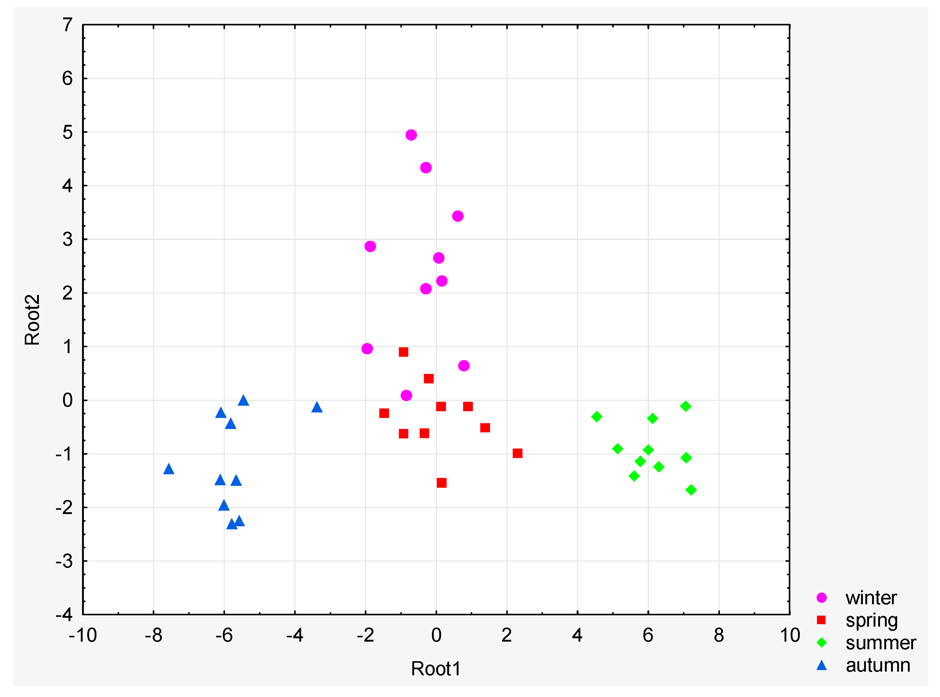
At the final stage of calculations, the discriminant analysis (DA) was performed on the data using a standard stepwise method. This made it possible to build a model containing 13 water quality parameters that were used to characterize the temporal variability of the physical and chemical composition of water in the basin (Table 3). The discriminant analysis allows for building orthogonal functions with a cumulative variance of 97% in the event of temporal variability. The DA was performed on raw data after splitting the dataset into four groups (spring, summer, autumn, and winter) based on the results of the CA and PCA. Since the grouping variable had four categories, three discriminant functions (DF) were obtained (Table 4). Only two of them were statistically significant (p < 0.01). The DA identified six variables (DO, SS, pH, N-K, N, and P-PO4) as the most important discriminating variables (Table 5). The first discriminant function is weighted most heavily by the SS and N (Table 6). The second function seems to be marked mostly by P-PO4 and EC. The graphical presentation of DA results is shown in Figure 4. It can be stated that we obtain discrimination between the summer and autumn seasons by means of the first discriminant function. However, the second discriminant function seems to distinguish between winter and autumn seasons.
4. Discussion
The HCA analysis allowed for the identification of two clusters represented as low pollution and moderate pollution levels. Cluster 1 was formed by sites 4, 7, 9, and 10, while the other six sites were assigned to cluster 2. Stations 7 and 10 were located on the tributaries of the river (Figure 1) in areas with no industrial activity and with dispersed single-family housing. Various factors influence the water quality in these stations: agricultural practices, animal husbandry, and domestic sewage [10,20]. Stations 4 and 9 were located in the city of Lublin in the area of intensive road infrastructure and clustered housing development. In these stations, increased levels of pollution can result from surface runoff and domestic sewage discharge. Increased levels of river pollution in these locations are due to seasonal human activity, which can lead to eutrophication. In stations located in the Bystrzyca river basin, increases are observed in pollution concentrations; however, they are not constant. Cyclical changes in rainfall intensity and human agricultural activity contribute to the formation of clear differences in water quality depending on the season of the year [63,64,65].
The low level of pollution in spring is probably due to dilution of melting snow by runoff. The relatively low concentration values of the tested parameters in spring are mainly caused by dilution. In turn, the very low level of pollution in summer is due to heavy rainfall and the uptake of nutrients by plants. The use of large amounts of fertilizers in agricultural areas and the use of salt for de-icing of roads in urban areas may contribute to increased concentrations of pollutants. Strong seasonal variation in pH, DO, BOD, and COD may result from photosynthesis, hydrological pollution, and natural chemical processes [22,23,66,67,68]. High TOC concentrations should be considered a result of the dissolution of minerals containing calcium carbonate, which occurs in loess soils [51,55]. The high SS content causes a reduction in DO, which affects the quality of water in the river. The high level of water quality parameters points to causes of pollution, such as withered and decaying plants, mineral acids, or agricultural and industrial waste discharged into the river [69,70]. For this reason, the highest values of pollution parameters were observed in autumn. Other studies show that the highest pollution values occurred in spring as a result of surface runoff. This indicates that, as a result of soil erosion processes, pollutants are accumulated in rivers [71]. Intensive erosion in highlands occurs during tillage and heavy rainfall. The frequency of pollution and soil erosion intensity depend on the land use and the type and manner of performing agricultural works [72,73].
The sources of pollution in a river basin can be identified on the basis of factor analysis [28,69,71]. The PCA used in the work did not allow for determining the spatial variability of the tested water quality parameters. No differences were found between stations located at sewage discharge points and in other places. This is due to the fact that point pollution is often superimposed on area pollution. The HCA and PCA/FA analysis showed that both sources of pollution are at a comparably high level. This suggests that potentially harmful substances may be of natural or anthropogenic origin, or both [74]. In addition, some man-made compounds also occur in natural conditions, e.g., gypsum [20,64,66]. In the studied Bystrzyca river catchment, water is only moderately polluted by agricultural practices or municipal sewage. The lowest quality water was found at station 4. This was due to surface runoff from the city and discharge from the municipal sewage treatment plant. At station 5, however, a significant improvement in water quality was observed, which reveals the river’s self-cleaning ability [69]. Previous studies show that heavy metal concentrations were characterized by very low values [57].
5. Conclusions
Chemometric techniques are a useful tool to describe water quality and its spatial and temporal variability caused by natural and anthropogenic factors. The cluster analysis allowed for the identification of two clusters. One included four stations with a moderate pollution level, while the other comprised six stations with a low level of water pollution. The principal component analysis did not provide an unambiguous assessment of the spatial variability of water quality in the basin and the identification of hot spots. This is due to the simultaneous occurrence of area and point source pollution in the analyzed basin with a similar effect on water quality. Analyses carried out using PCA and DA showed statistically significant temporal variability between the study seasons. In the Bystrzyca river basin, we get differences between the summer and autumn seasons using the first discriminant function. With the second discriminant function, we get differences between winter and autumn seasons. The differences between the seasons are due to human activity, the type of agricultural treatment, and agricultural runoff. The main task of managers is to limit the frequency and intensity of erosion. This can be achieved by introducing tree cover and good agricultural practices, and by limiting surface sealing. This study can help the water resources management in the region.
The analyzed surface waters had the best quality in the summer season, and the worst in the autumn season. The samples were characterized by very high EC, SS, and P-PO4 concentrations and the water quality did not meet the standards of good ecological status. Excess ortophosphate (P-PO4) from feed, fertilizers, and industrial waste, is an underlying factor contributing to the deterioration of water ecosystems. In turn, electrical conductivity (EC) and suspended solids (SS) as water salinity indicators reflect the impact of urbanization and soil erosion.
Author Contributions
Conceptualization, A.G.; Data curation, A.G.; Formal analysis, A.G. and U.B.-M.; Investigation, A.G.; Methodology, A.G. and U.B.-M.; Software, U.B.-M.; Supervision, A.G.; Visualization, A.G. and U.B.-M.; Writing—original draft, A.G. and U.B.-M.; Writing—review and editing, A.G. and U.B.-M. All authors have read and agreed to the published version of the manuscript.
Funding
Publication is funded by the Polish National Agency for Academic Exchange under the International Academic Partnerships Programme from the project, Organization of the 9th International Scientific and Technical Conference entitled Environmental Engineering, Photogrammetry, Geoinformatics—Modern Technologies and Development Perspectives.
Conflicts of Interest
The authors declare no conflict of interest.
References
- Pastuszak, M.; Igras, J. Temporal and Spatial Differences in Emission of Nitrogen and Phosphorus from Polish Territory to the Baltic Sea; INUG: Puławy, Poland, 2012; pp. 1–452. [Google Scholar]
- Szalińska, E. Water quality and management changes over the history of Poland. Bull. Environ. Contam. Toxicol. 2018, 100, 26–31. [Google Scholar] [CrossRef] [PubMed]
- Wijesiri, B.; Deilami, K.; Goonetilleke, A. Evaluating the relationship between temporal changes in land use and resulting water quality. Environ. Pollut. 2018, 234, 480–486. [Google Scholar] [CrossRef] [PubMed]
- Xu, G.; Li, P.; Lu, K.; Tantai, Z.; Zhang, J.; Ren, Z.; Wang, X.; Yu, K.; Shi, P.; Cheng, Y. Seasonal changes in water quality and its main influencing factors in the Dan River basin. Catena 2019, 173, 131–140. [Google Scholar] [CrossRef]
- Mainali, J.; Chang, H. Landscape and anthropogenic factors affecting spatial patterns of water quality trends in a large river basin, South Korea. J. Hydrol. 2018, 564, 26–40. [Google Scholar] [CrossRef]
- Melland, A.R.; Fenton, O.; Jordan, P. Effects of agricultural land management changes on surface water quality: A review of meso-scale catchment research. Environ. Sci. Policy 2018, 84, 19–25. [Google Scholar] [CrossRef]
- Barzegar, R.; Asghari Moghaddam, A.; Soltani, S.; Baomid, N.; Tziritis, E.; Adamowski, J.; Inam, A. Natural and anthropogenic origins of selected trace elements in the surface waters of Tabriz area, Iran. Environ. Earth Sci. 2019, 78, 254. [Google Scholar] [CrossRef]
- Dąbrowska, J.; Lejcuś, K.; Kuśnierz, M.; Czamara, A.; Kamińska, J.; Lejcuś, I. Phosphate dynamics in the drinking water catchment area of the Dobromierz Reservoir. Desalin. Water Treat. 2016, 57, 25600–25609. [Google Scholar] [CrossRef]
- Liu, C.W.; Lin, K.H.; Kuo, Y.M. Application of factor analysis in the assessment of groundwater quality in a black foot disease area in Taiwan. Sci. Total Environ. 2003, 313, 77–89. [Google Scholar] [CrossRef]
- Varol, M.; Gökot, B.; Bekleyen, A.; Sen, B. Spatial and temporal variations in surface water quality of the dam reservoirs in the Tigris River basin, Turkey. Catena 2012, 92, 11–21. [Google Scholar] [CrossRef]
- Mena-Rivera, L.; Salgado-Silva, V.; Benavides-Benavides, C.; Coto-Campos, J.; Swinscoe, T. Spatial and seasonal surface water quality assessment in a tropical urban catchment: Burío River, Costa Rica. Water 2017, 9, 558. [Google Scholar] [CrossRef] [Green Version]
- Parizi, S.H.; Samani, N. Geochemical evolution and quality assessment of water resources in the Sarcheshmeh copper mine area (Iran) using multivariate statistical techniques. Environ. Earth Sci. 2013, 69, 1699–1718. [Google Scholar] [CrossRef]
- Kaźmierska, A.; Szelag-Wasilewska, E. Evaluation of spatial and temporal variations in the quality of water: A case study of small stream in Poland. J. Ecology Environ. Sci. 2015, 6, 137–142. [Google Scholar]
- Kowalik, T.; Kanownik, W.; Bogdał, A.; Policht-Latawiec, A. Effect of change of small upland catchment use on surface water quality course. Rocz. Ochr. Srodowiska 2015, 16, 223–238. [Google Scholar]
- Sojka, M.; Jaskuła, J.; Wicher-Dysarz, J. Assessment of biogenic compounds elution from the Główna River Catchment in the years 1996–2009. Rocz. Ochr. Srodowiska 2016, 18, 815–830. (In Polish) [Google Scholar]
- Liberacki, D.; Szafrański, C. Contents of biogenic components in surface waters of small catchments in the Zielonka Forest. Rocz. Ochr. Srodowiska 2008, 10, 181–192. [Google Scholar]
- Miernik, W.; Wałęga, A. Anthropogenic influence on the quality of water in the Prądnik river. Environ. Prot. Eng. 2008, 34, 103–108. [Google Scholar]
- Heathwaite, A.L.; Quinn, P.F.; Hewett, C.J.M. Modelling and managing critical source areas of diffuse pollution from agricultural land using flow connectivity simulation. J. Hydrol. 2005, 304, 446–461. [Google Scholar] [CrossRef]
- Spiess, E. Nitrogen, phosphorus and potassium balances and cycles of Swiss agriculture from 1975 to 2008. Nutr. Cycl. Agroecosyst. 2011, 91, 351–365. [Google Scholar] [CrossRef]
- Bu, H.; Tan, X.; Li, S.; Zhang, Q. Temporal and spatial variations of water quality in the Jinshui River of the South Qinling Mts., China. Ecotoxicol. Environ. Saf. 2010, 73, 907–913. [Google Scholar] [CrossRef]
- Kozak, J.; Ostapowicz, K.; Bytnerowicz, A.; Wyżga, B. The Carpathians: Integrating nature and society towards sustainability. In Environmental Science Engineering; Springer: Berlin, Germany, 2013. [Google Scholar]
- Kurunc, A.; Ersahin, S.; Sonmez, N.K.; Kaman, H.; Uz, I.; Uz, B.Y.; Aslan, G.E. Seasonal changes of spatial variation of some groundwater quality variables in a large irrigated coastal Mediterranean region of Turkey. Sci. Total Environ. 2016, 554, 53–63. [Google Scholar] [CrossRef]
- Wang, J.; Hu, M.; Hang, F.; Gao, B. Influential factors detection for surface water quality with geographical detectors in China. Stoch. Env. Res. Risk Assess. 2018, 32, 2633–2645. [Google Scholar] [CrossRef]
- Ngoye, E.; Machiwa, J.F. The influence of land-use patterns in the Ruvu river watershed on water quality in the river system. Phys. Chem. Earth Parts A/B/C 2004, 29, 1161–1166. [Google Scholar] [CrossRef]
- Orzepowski, W.; Pulikowski, K. Magnesium, calcium, potassium and sodium content in groundwater and surface water in arable lands in the commune of Kąty Wrocławskie. J. Elementol. 2008, 13, 605–614. [Google Scholar]
- Astel, A.; Biziuk, M.; Przyjazny, A.; Namieśnik, J. Chemometrics in monitoring spatial and temporal variations in drinking water quality. Water Res. 2006, 40, 1706–1716. [Google Scholar] [CrossRef] [PubMed]
- Gamble, A.; Babbar-Sebens, M. On the use of multivariate statistical methods for combining in-stream monitoring data and spatial analysis to characterize water quality conditions in the White River, Indiana, USA. Environ. Monit. Assess. 2012, 184, 845–875. [Google Scholar] [CrossRef]
- Li, S.; Li, J.; Zhang, Q. Water quality assessment in the rivers along the water conveyance system of the Middle Route of the South to North Water Transfer Project (China) using multivariate statistical techniques and receptor modeling. J. Hazard. Mater. 2011, 195, 306–317. [Google Scholar] [CrossRef]
- López-López, J.A.; Mendiguchían, C.; García-Vargasn, M.; Morenon, C. Multi-way analysis for decadal pollution trends assessment: The Guadalquivir River estuary as a case study. Chemosphere 2014, 111, 47–54. [Google Scholar] [CrossRef]
- Mostafaei, A. Application of multivariate statistical methods and water-quality index to evaluation of water quality in the Kashkan River. Environ. Manag. 2014, 53, 865–881. [Google Scholar] [CrossRef]
- Osman, R.; Saim, N.; Juahir, H.; Abdullah, M. Chemometric application in identifying sources of organic contaminants in Langat river basin. Environ. Monit. Assess. 2012, 184, 1001–1014. [Google Scholar] [CrossRef]
- Wang, Y.B.; Liu, C.W.; Liao, P.Y.; Lee, J.J. Spatial pattern assessment of river water quality: Implications of reducing the number of monitoring stations and chemical parameters. Environ. Monit. Assess. 2014, 186, 1781–1792. [Google Scholar] [CrossRef]
- Khan, M.Y.A.; Gani, K.M.; Chakrapani, G.J. Assessment of surface water quality and its spatial variation. A case study of Ramganga River, Ganga Basin, India. Arab. J. Geosci. 2016, 9, 1–9. [Google Scholar]
- Kumarasamy, P.; James, R.A.; Dahms, H.U.; Byeon, C.W.; Ramesh, R. Multivariate water quality assessment from the Tamiraparani river basin, Southern India. Environ. Earth Sci. 2014, 71, 2441–2451. [Google Scholar] [CrossRef]
- Phung, D.; Huang, C.; Rutherford, S.; Dwirahmadi, F.; Chu, C.; Wang, X.; Nguyen, M.; Nguyen, N.H.; Manh Do, C.; Nguyen, T.H.; et al. Temporal and spatial assessment of river surface water quality using multivariate statistical techniques: A study in Can Tho City, a Mekong Delta area, Vietnam. Environ. Monit. Assess. 2015, 187, 1–13. [Google Scholar] [CrossRef]
- Sharma, M.; Kansal, A.; Jain, S.; Sharma, P. Application of multivariate statistical techniques in determining the spatial temporal water quality variation of Ganga and Yamuna Rivers present in Uttarakhand State, India. Water Qual. Expo. Health 2015, 7, 567–581. [Google Scholar] [CrossRef]
- Thuong, N.T.; Yoneda, M.; Matsui, Y. Does embankment improve quality of a river? A case study in To Lich River inner city Hanoi, with special reference to heavy metals. J. Environ. Prot. 2013, 4, 361–370. [Google Scholar] [CrossRef] [Green Version]
- Varekar, V.S.; Karmakar, J.R.; Ghosh, N.C. Design of sampling locations for river water quality monitoring considering seasonal variation of point and diffuse pollution loads. Environ. Monit. Assess. 2015, 187, 376. [Google Scholar] [CrossRef]
- Barakat, A.; El Baghdadi, M.; Rais, J.; Aghezzaf, B.; Slassi, M. Assessment of spatial and seasonal water quality variation of Oum Er Rbia River (Morocco) using multivariate statistical techniques. Int. Soil. Water Cons. Res. 2016, 4, 284–292. [Google Scholar] [CrossRef]
- Sun, X.; Zhang, H.; Zhong, M.; Wang, Z.; Liang, X.; Huang, T.; Huang, H. Analyses on the Temporal and Spatial Characteristics of Water Quality in a Seagoing River using Multivariate Statistical Techniques: A Case Study in the Duliujian River, China. Int. J. Environ. Res. Public Health 2019, 16, 1020. [Google Scholar] [CrossRef] [Green Version]
- Zhang, W.; Jin, X.; Liu, D.; Lang, C.; Shan, B. Temporal and spatial variation of nitrogen and phosphorus and eutrophication assessment for a typical arid river—Fuyang River in northern China. J. Environ. Sci. 2017, 55, 41–48. [Google Scholar] [CrossRef]
- Zhang, X.; Wang, Q.; Liu, Y.; Wu, J.; Yu, M. Application of multivariate statistical techniques in the assessment of water quality in the Southwest New Territories and Kowloon, Hong Kong. Environ. Monit. Assess. 2011, 173, 17–27. [Google Scholar] [CrossRef]
- Ismail, A.H.; Abed, B.S.; Abdul-Qader, S. Application of multivariate statistical techniques in the surface water quality assessment of Tigris River at Baghdad stretch, Iraq. J. Univ. Babylon 2014, 22, 450–462. [Google Scholar]
- Kausar, F.; Qadir, A.; Ahmad, S.R.; Baqar, M. Evaluation of surface water quality on spatiotemporal gradient using multivariate statistical techniques: A case study of River Chenab, Pakistan. Pol. J. Environ. Stud. 2019, 28, 2645–2657. [Google Scholar] [CrossRef]
- Malik, R.N.; Hashmi, M.Z. Multivariate statistical techniques for the evaluation of surface water quality of the Himalayan foothills streams, Pakistan. Appl. Water Sci. 2017, 7, 2817–2830. [Google Scholar] [CrossRef]
- Sojka, M.; Siepak, M.; Zioła, A.; Frankowski, M.; Murat-Błażejewska, S.; Siepak, J. Application of multivariate statistical techniques to evaluation of water quality in the Mała Wełna River (Western Poland). Environ. Monit. Assess. 2008, 147, 159–170. [Google Scholar] [CrossRef]
- Glińska-Lewczuk, K.; Gołaś, I.; Koc, J.; Gotkowska-Płachta, A.; Karnisz, M.; Rochwerger, A. The impact of urban areas on the water quality gradient along a lowland river. Environ. Monit. Assess. 2016, 188, 624–640. [Google Scholar] [CrossRef]
- Bogdał, A.; Wałęga, A.; Kowalik, T.; Cupak, A. Assessment of the impact of forestry and settlement-forest use of the catchments on the parameters of surface water quality: Case studies for Chechło Reservoir catchment, southern Poland. Water 2019, 11, 964. [Google Scholar] [CrossRef] [Green Version]
- Czekaj, J.; Jakóbczyk-Karpierz, S.; Rubin, H. Identification of nitrate sources in groundwater and potential impact on drinking water reservoir (Goczałkowice reservoir, Poland). Phys. Chem. Earth Parts A/B/C 2016, 94, 35–46. [Google Scholar] [CrossRef]
- Siepak, M.; Sojka, M. Application of multivariate statistical approach to identify trace elements sources in surface waters: A case study of Kowalskie and Stare Miasto reservoirs. Environ. Monit. Assess. 2017, 189, 364–374. [Google Scholar] [CrossRef] [Green Version]
- Grzywna, A.; Jóźwiakowski, K.; Gizińska-Górna, M.; Marzec, M.; Mazur, A.; Obroślak, R. Analysis of ecological status of surface waters in the Bystrzyca river in Lublin. J. Ecol. Eng. 2016, 17, 203–207. [Google Scholar] [CrossRef]
- Grzywna, A.; Sender, J.; Bronowicka-Mielniczuk, U. Analysis of the ecological status of surface waters in the Region of the Lublin conurbation. Rocz. Ochr. Środowiska 2017, 19, 439–450. [Google Scholar]
- Skowron, P.; Igras, J. Anthropogenic sources of nitrogen in the Bystrzyca. Przem. Chem. 2012, 91, 970–977. (In Polish) [Google Scholar]
- Skowron, P.; Igras, J. Anthropogenic sources of phosphorus in the catchment of the Bystrzyca river. Preliminary analysis of the share of agriculture in the process of water pollution. Przem. Chem. 2013, 92, 787–790. (In Polish) [Google Scholar]
- Skowron, P.; Skowrońska, M.; Bronowicka-Mielniczuk, U.; Filipek, T.; Igras, J.; Kowalczyk-Juśko, A.; Krzepiło, A. Anthropogenic sources of potassium in surface water: The case study of the Bystrzyca river catchment, Poland. Agric. Ecosys. Environ. 2018, 265, 454–460. [Google Scholar] [CrossRef]
- Czarnecka, H. Atlas Podziału Hydrograficznego Polski; PWN: Warszawa, Poland, 2005. [Google Scholar]
- Wojewódzki Inspektorat Ochrony Środowiska. Wartości Minimalne, Maksymalne i Średnie Wyników w Monitorowanych Jcwp w 2016 Roku. Available online: http://www.wios.lublin.pl/srodowisko/monitoring-wod/ocena-jakosci-wod-rzek/ (accessed on 24 December 2019).
- Oksanen, J.; Blanchet, F.G.; Friendly, M.; Kindt, R.; Legendre, P.; Mc Glinn, D.; Minchin, P.R.; O’Hara, R.B.; Simpson, G.L.; Solymos, P.; et al. Vegan: Community Ecology Package ver. 2.4-6; CRAN, 2018. Available online: https://cran.r-project.org/web/packages/vegan/index.html (accessed on 24 December 2019).
- R Core Team. R: A Language and Environment for Statistical Computing; R Foundation for Statistical Computing: Vienna, Austria, 2017. [Google Scholar]
- Borcard, D.; Gillet, F.; Legendre, P. Numerical Ecology with R; Springer: New York, NY, USA, 2011. [Google Scholar]
- Decrem, M.; Spiess, E.; Richner, W.; Herzog, F. Impact of Swiss agricultural policies on nitrate leaching from arable land. Agron. Sustain. Dev. 2007, 27, 243–253. [Google Scholar] [CrossRef]
- Pérez-Gutiérrez, J.D.; Paz, J.O.; Tagert, M.L.M. Seasonal water quality changes in on-farm water storage systems in a south-central U.S. agricultural watershed. Agric. Water Manag. 2017, 187, 131–139. [Google Scholar] [CrossRef] [Green Version]
- Viswanathan, C.V.; Jiang, Y.; Berg, M.; Hunkeler, D.; Schirmer, M. An integrated spatial snap-shot monitoring method for identifying seasonal changes and spatial changes in surface water quality. J. Hydrol. 2016, 539, 567–576. [Google Scholar] [CrossRef] [Green Version]
- Adeogun, A.O.; Babatunde, T.A.; Chukwuka, A.V. Spatial and temporal variations in water and sediment quality of Ona river, Ibadan, Southwest Nigeria. Eur. J Scien. Res. 2012, 74, 186–204. [Google Scholar]
- Varol, M.; Gökot, B.; Bekleyen, A.; Şen, B. Water quality assessment and apportionment of pollution sources of Tigris River (Turkey) using multivariate statistical techniques—A case study. River Res. Appl. 2012, 28, 1428–1438. [Google Scholar] [CrossRef]
- Guo, H.; Wang, Y. Hydrogeochemical processes in shallow quaternary aquifers from the northern part of the Datong Basin, China. Appl. Geochem. 2004, 19, 19–27. [Google Scholar] [CrossRef]
- Olias, M.; Ceron, J.C.; Moral, F.; Ruiz, F. Water quality of the Guadiamar River after the Aznalcollar spill (SW Spain). Chemosphere 2006, 62, 213–225. [Google Scholar] [CrossRef]
- Ravichandran, S. Hydrological influences on the water quality trends in Tamiraparani Basin, south India. Environ. Monit. Assess. 2003, 87, 293–309. [Google Scholar] [CrossRef] [PubMed]
- Kannel, P.R.; Lee, S.; Lee, Y.S. Assessment of spatial–temporal patterns of surface and ground water qualities and factors influencing management strategy of groundwater system in an urban river corridor of Nepal. J. Environ. Manag. 2008, 86, 595–604. [Google Scholar] [CrossRef] [PubMed]
- Sun, W.; Xia, C.; Xu, M.; Guo, J.; Sun, G. Application of modified water quality indices as indicators to assess the spatial and temporal trends of water quality in the Dongjiang River. Ecol. Indic. 2016, 66, 306–312. [Google Scholar] [CrossRef]
- Kowalkowski, T.; Zbytniewski, R.; Szpejna, J.; Buszewski, B. Application of chemometrics in river water classification. Water Res. 2006, 40, 744–752. [Google Scholar] [CrossRef]
- Absalon, D.; Matysik, M. Changes in water quality and runoff in the Upper Oder River Basin. Geomorphology 2007, 92, 106–118. [Google Scholar] [CrossRef]
- Mazur, A. Quantity and quality of surface and subsurface runoff from an eroded loess slope used for agricultural purposes. Water 2018, 10, 1132. [Google Scholar] [CrossRef] [Green Version]
- Caccia, V.G.; Boyer, G.N. Spatial patterning of water quality in Biscayne Bay, Florida as a function of land use and water management. Mar. Pollut. Bull. 2005, 50, 1416–1429. [Google Scholar] [CrossRef]
Figure 1.
The hydrographic network of the Bystrzyca river basin.

Figure 2.
A dendrogram of the hierarchical cluster analysis based on the Euclidean measure and Ward’s method: (a) measuring stations, (b) measuring stations and seasons.
Figure 2.
A dendrogram of the hierarchical cluster analysis based on the Euclidean measure and Ward’s method: (a) measuring stations, (b) measuring stations and seasons.


Figure 3.
Results of the principal component analysis for: (a) measuring stations, (b) seasons.


Figure 4.
Results of the discriminant analysis (DA) for sample collection seasons.


Table 1.
Location of the station in the Bystrzyca river basin.
| No. | Station | River | Outlet (km) | Flow (m−3·s−1) |
|---|---|---|---|---|
| 1 | Kiełczewice | Bystrzyca Lublin | 60 | 0.4 |
| 2 | Osmolice | 48 | 1.0 | |
| 3 | Zemborzyce | 38 | 2.2 | |
| 4 | Hajdów | 20 | 3.8 | |
| 5 | Spiczyn | 3 | 4.9 | |
| 6 | Iżyce | Kosarzewka | 3 | 0.9 |
| 7 | Krężnica | Krężniczanka | 5 | 0.9 |
| 8 | Głusk | Czerniejówka | 7 | 0.7 |
| 9 | Zamek | Czechówka | 1 | 0.2 |
| 10 | Pliszczyn | Ciemięga | 4 | 0.6 |
Table 2.
Season-specific values of the physical and chemical parameters.
| Seasons | DO | BOD | COD | TOC | EC | SS | pH | N-NH4 | N-K | N-NO3 | N | P-PO4 | P | |
|---|---|---|---|---|---|---|---|---|---|---|---|---|---|---|
| Unit | mgO2/L | mgO2/L | mgO2/L | mgC/L | μS/cm | mg/L | - | mg/L | mg/L | mg/L | mg/L | mg/L | mg/L | |
| Winter | Mean | 9.89 | 2.8 | 18 | 5.07 | 533.5 | 386.13 | 8.03 | 0.142 | 1.163 | 2.252 | 3.291 | 0.194 | 0.263 |
| SD | 0.351 | 0.636 | 5.578 | 1.365 | 67.605 | 63.344 | 0.082 | 0.054 | 0.169 | 0.698 | 0.686 | 0.056 | 0.125 | |
| Min | 9.3 | 1.9 | 11 | 3.0 | 393 | 261 | 7.9 | 0.10 | 0.9 | 1.5 | 2.4 | 0.1 | 0.13 | |
| Max | 10.5 | 3.7 | 28 | 7.4 | 625 | 457 | 8.2 | 0.25 | 1.4 | 3.47 | 4.74 | 0.3 | 0.44 | |
| Spring | Mean | 9.77 | 2.63 | 15.70 | 4.10 | 561.10 | 382.56 | 7.92 | 0.16 | 1.30 | 1.93 | 3.11 | 0.13 | 0.20 |
| SD | 0.769 | 0.690 | 4.715 | 1.046 | 61.167 | 47.006 | 0.116 | 0.065 | 0.192 | 0.628 | 0.708 | 0.055 | 0.059 | |
| Min | 8.5 | 1.9 | 9.0 | 2.1 | 490.0 | 300.0 | 7.7 | 0.1 | 1.0 | 1.3 | 1.8 | 0.1 | 0.1 | |
| Max | 10.8 | 4 | 23 | 5.8 | 656 | 434 | 8.04 | 0.32 | 1.6 | 3.1 | 4 | 0.24 | 0.31 | |
| Summer | Mean | 8.50 | 1.89 | 12.40 | 2.78 | 482.00 | 343.67 | 7.74 | 0.07 | 0.96 | 1.47 | 2.31 | 0.08 | 0.16 |
| SD | 0.552 | 0.515 | 3.836 | 1.022 | 37.880 | 30.952 | 0.137 | 0.067 | 0.208 | 0.576 | 0.497 | 0.037 | 0.052 | |
| Min | 7.6 | 1.4 | 8.0 | 1.1 | 445.0 | 305.0 | 7.5 | 0.0 | 0.7 | 0.7 | 1.5 | 0.01 | 0.1 | |
| Max | 9.1 | 3 | 20 | 4.4 | 563 | 402 | 7.89 | 0.25 | 1.19 | 2.46 | 2.95 | 0.173 | 0.26 | |
| Autumn | Mean | 10.80 | 3.53 | 19.40 | 5.47 | 658.60 | 419.33 | 8.13 | 0.27 | 1.44 | 2.26 | 3.86 | 0.15 | 0.27 |
| SD | 0.655 | 0.778 | 4.274 | 1.398 | 95.690 | 62.942 | 0.031 | 0.052 | 0.195 | 0.517 | 0.761 | 0.043 | 0.069 | |
| Min | 9.9 | 2.6 | 15.0 | 2.6 | 500.0 | 344.0 | 8.1 | 0.2 | 1.2 | 1.5 | 3.0 | 0.1 | 0.2 | |
| Max | 12.1 | 4.5 | 28 | 6.9 | 802 | 522 | 8.2 | 0.34 | 1.88 | 3.2 | 5.24 | 0.24 | 0.37 |
Table 3.
Matrix of factor loadings calculated on the basis of water quality parameters.
| Parameter | PC1 | PC2 | PC3 |
|---|---|---|---|
| DO | −0.73 b | 0.07 | −0.09 |
| BOD | −0.72 b | −0.01 | −0.49 |
| COD | −0.59 b | −0.44 | 0.21 |
| TOC | −0.67 b | −0.01 | −0.67 b |
| EC | −0.85 a | −0.26 | 0.27 |
| SS | −0.79 a | −0.22 | 0.24 |
| pH | −0.78 a | 0.23 | 0.02 |
| N-NH4 | −0.88 a | −0.19 | −0.02 |
| N-K | −0.79 a | −0.37 | 0.05 |
| N-NO3 | −0.54 b | 0.70 b | 0.38 |
| N | −0.73 b | 0.44 | 0.32 |
| P-PO4 | −0.46 | 0.60 b | −0.32 |
| P | −0.76 a | −0.11 | −0.03 |
| Eigenvalue | 6.81 | 1.61 | 1.22 |
| Variance % | 52.40 | 12.37 | 9.37 |
| Cumulative variance % | 52.40 | 64.77 | 74.14 |
a Strongly correlated factor loadings; b Medium correlated factor loadings.
Table 4.
Wilk’s lambda and chi-square test for the discriminant analysis of temporal variation.
| Discriminant Factor | Eigenvalue | R | Wilk’s Lambda | Chi-Square | p-Level |
|---|---|---|---|---|---|
| 0 | 19.50412 | 0.975310 | 0.009453 | 142.1747 | 0.000000 |
| 1 | 2.26927 | 0.833139 | 0.193817 | 50.0456 | 0.001397 |
| 2 | 0.57818 | 0.605276 | 0.633641 | 13.9163 | 0.237659 |
Table 5.
The discriminant analysis of water quality parameters measured at 10 stations, variable grouping—season.
Table 5.
The discriminant analysis of water quality parameters measured at 10 stations, variable grouping—season.
| Parameter | Wilks’ Lambda | Partial Wilks’ Lambda | F-Remove | p-Level | Tolerance |
|---|---|---|---|---|---|
| DO | 0.013783 | 0.685831 | 3.664690 | 0.026379 | 0.606812 |
| BOD | 0.011303 | 0.836268 | 1.566316 | 0.223442 | 0.253237 |
| COD | 0.012709 | 0.743786 | 2.755789 | 0.064460 | 0.432741 |
| OWO | 0.012701 | 0.744268 | 2.748818 | 0.064916 | 0.210628 |
| EC | 0.012914 | 0.731978 | 2.929291 | 0.054131 | 0.151339 |
| SS | 0.014432 | 0.654958 | 4.214523 | 0.015763 | 0.165511 |
| pH | 0.018440 | 0.512605 | 7.606565 | 0.000962 | 0.448278 |
| N-NH4 | 0.009703 | 0.974196 | 0.211903 | 0.887158 | 0.383435 |
| N-K | 0.014939 | 0.632754 | 4.643150 | 0.010690 | 0.239602 |
| N-NO3 | 0.009785 | 0.966057 | 0.281081 | 0.838510 | 0.177250 |
| N | 0.013395 | 0.705667 | 3.336785 | 0.036190 | 0.152398 |
| P-PO4 | 0.015121 | 0.625147 | 4.796987 | 0.009324 | 0.387294 |
| P | 0.011541 | 0.819024 | 1.767728 | 0.180194 | 0.450575 |
Table 6.
Standardized canonical discriminant function coefficients.
| Root1 | Root2 | |
|---|---|---|
| DO | −0.638 | 0.052 |
| BOD | −0.206 | −0.491 |
| COD | −0.355 | 0.656 |
| OWO | −0.971 | 0.442 |
| EC | −0.483 | −1.414 |
| SS | 1.371 | 0.584 |
| pH | −0.979 | 0.059 |
| N-NH4 | −0.110 | −0.281 |
| N-K | −0.506 | 0.397 |
| N-NO3 | 0.383 | −0.134 |
| N | −1.348 | 0.502 |
| P-PO4 | 0.649 | 0.903 |
| P | 0.309 | −0.266 |
© 2020 by the authors. Licensee MDPI, Basel, Switzerland. This article is an open access article distributed under the terms and conditions of the Creative Commons Attribution (CC BY) license (http://creativecommons.org/licenses/by/4.0/).
Share and Cite
MDPI and ACS Style
Grzywna, A.; Bronowicka-Mielniczuk, U. Spatial and Temporal Variability of Water Quality in the Bystrzyca River Basin, Poland. Water 2020, 12, 190. https://doi.org/10.3390/w12010190
AMA Style
Grzywna A, Bronowicka-Mielniczuk U. Spatial and Temporal Variability of Water Quality in the Bystrzyca River Basin, Poland. Water. 2020; 12(1):190. https://doi.org/10.3390/w12010190
Chicago/Turabian StyleGrzywna, Antoni, and Urszula Bronowicka-Mielniczuk. 2020. "Spatial and Temporal Variability of Water Quality in the Bystrzyca River Basin, Poland" Water 12, no. 1: 190. https://doi.org/10.3390/w12010190
Note that from the first issue of 2016, this journal uses article numbers instead of page numbers. See further details here.