Characterization of Kyagar Glacier and Lake Outburst Floods in 2018 Based on Time-Series Sentinel-1A Data


1
Key Laboratory of Digital Earth Science, Institute of Remote Sensing and Digital Earth, Chinese Academy of Sciences, No. 9 Dengzhuang South Road, Beijing 100094, China
2
University of Chinese Academy of Sciences, Beijing 100049, China
3
Hainan Key Laboratory of Earth Observation, Institute of Remote Sensing and Digital Earth, Chinese Academy of Sciences, Sanya 572029, China
*
Author to whom correspondence should be addressed.
Water 2020, 12(1), 184; https://doi.org/10.3390/w12010184
Submission received: 25 November 2019
/
Revised: 26 December 2019
/
Accepted: 6 January 2020
/
Published: 9 January 2020
(This article belongs to the Section Water Resources Management, Policy and Governance)
Abstract
:Early recognition of glacial lake outburst floods (GLOFs) is required for timely and cost-effective remedial efforts to be implemented. Although the formation of ice-dammed lakes is known to begin as a pond or river that was blocked by ice from the glacier terminus, the relationship between glacier dynamics and lake development is not well understood. Using a time-series of Sentinel-1A synthetic aperture radar (SAR) data acquired just before and after the lake outburst event in 2018, information is presented on the dynamic characteristics of Kyagar Glacier and its ice-dammed lake. Glacier velocity data derived from interferometry show that the glacier tongue experienced an accelerated advance (maximum velocity of 20 cm/day) just one month before the lake outburst, and a decreased velocity (maximum of 13 cm/day) afterward. Interferometric and backscattering properties of this region provide valuable insight into the diverse glaciated environment. Furthermore, daily temperature and total precipitation data derived from the ECMWF re-analysis (ERA)Interim highlight the importance of the sustained high-temperature driving force, supporting empirical observations from previous studies. The spatial and temporal resolution offered by the Sentinel-1A data allows variations in the glacier surface motion and lake evolution to be detected, meaning that the interaction mechanism between the glacial lake and the associated glacier can be explored. Although the glacier surge provided the boundary conditions favorable for lake formation, the short-term high temperatures and precipitation caused the melting of ice dams and also a rapid increase in the amount of water stored, which accelerated the potential for a lake outburst.
1. Introduction
In the context of global climate warming, glaciers have been retreating and thinning markedly in high mountain areas. This has led to the formation of numerous glacial lakes impounded by end-moraines, glacier tongues, or stagnating glacier snouts [1,2]. The abundant storage and then release of water from glacial lakes can cause hazardous flooding, commonly known as glacial lake outburst floods (GLOFs). GLOFs refer to sudden-onset outburst floods which may be induced by a moraine-dam failure, other outburst floods from a glacier, such as those caused by an ice dam failure, or the water suddenly released from a subglacial or englacial channel [3]. They are extremely complex and natural phenomena, which are characterized by the triggering mechanisms, lake hypsometry, the structure, geometry, and composition component of the surrounding dam, as well as the geology and topography where the flood pass through [4]. Generally, the peak discharge of these GLOFs is several orders of magnitude larger than that of floods induced by precipitation [5], which may greatly threaten life, property, and infrastructure in downstream areas. The floods can also impact glacier dynamics and cause substantial erosion to valley floors [6,7,8]. Consequently, early warning measures are very important in terms of reducing the risk to local communities.
Ice-dammed lakes are one typical kind of glacial lake formed by the advance of glaciers and dammed by glacier ice, regardless of their position relative to the glacier [9,10]. These lakes are short-lived, with a duration of only a few months, and are closely associated with glacier surging. Historical reports show that between the years 1533 and 2000, 71 GLOFs originated from ice breaches in the Karakoram Mountains, the region most seriously affected by lake outburst floods [9]. The Kyagar Glacier is a surge-type glacier situated on the northern slopes of the Karakoram Mountains. It has already caused GLOFs with devastating impacts on the downstream areas in the Yarkant River basin in northwest China [11,12,13]. The most recent lake outburst flood occurred on 10 August 2018 and had a flood discharge of 1570 m3/s, as measured at the Kuluklangan station on the lower reaches of the Yarkant River, and eventually poured approximately 35,000,000 m3 of water into the Shaksgam River. These serious disasters imply that, currently, it is necessary to carry out studies related to glacier motion, study how this motion influences glacial lakes and determine the mechanism causing lake outbursts.
Researchers have made substantial progress in identifying ice-dammed lakes and characterizing the dynamics of entire glacier systems at the present and during the Pleistocene, and including lakes at the base of ice sheets and ice caps, and in low-latitude regions of Asia and in Europe [3,4,14]. So far, three main approaches have been used for the estimation of glacier motion: in situ survey (e.g., GPS measurement), offset-tracking using optical data or synthetic aperture radar (SAR) data, and interferometric techniques using SAR data. Field measurement campaigns are often spatially and temporally hampered because most glaciers are in remote and desolate areas. Glacier flow velocity can be computed from optical data based on spatio-temporal intensity gradients [15]. However, this method is greatly limited in terms of the regular modeling of glaciers and glacial lake change patterns since most glaciated regions are characterized by bad weather, such as rain and snowfall, and also by cirrus clouds, all of which interfere with the imaging intensity to some extent. Besides, selecting the optimal cloudless data obtained over these regions is not an easy task. Under these conditions, SAR data has proved to be more suitable due to its being less affected by weather and illumination conditions [16,17]. SAR offset-tracking utilizes the backscattered intensity information of the radar image to determine the pixel offsets, which can be estimated to a small fraction of a pixel depending on the patch size used [18,19]. The advantages of differential SAR interferometry (DInSAR) over comparable techniques used to measure glacier velocities include the level of precision that can be achieved, which is typically around ±0.01 cm/day, and also that two-dimensional motion can be derived from a single SAR Single Look Complex (SLC) pair. In order to explore the proper glacier morphological conditions for lake development, Quincey et al. calculated glacier velocity using three tandem pairs of ERS-1 and ERS-2 data [20]. Using the same data, Capps et al. identified dynamic subglacial lakes and quantified changes in the vertical displacement of the glacier surface [21]. Sánchez-Gámez and Navarro made Interferometric Synthetic Aperture Radar (InSAR) observations of glacier motion in the southern Ellesmere ice caps (Canadian Arctic) using Sentinel-1 data [22]. Although the DInSAR technique has had some successful applications to the cryosphere, these studies only involved the movement of the glaciers, the role of glacier activity in the formation of glacial lakes and outburst floods has previously been unrecognized.
In this study, we conducted a detailed InSAR analysis characterizing a large mountain glacial system—The Kyagar Glacier. This glacier has a tendency to surge, leading to the formation of ice-dammed lakes and other changes over a time scale of a few days. To identify the mechanism behind the glacial lake outbursts, changes in the velocity distribution of the glacier were calculated from interferometry using a time series of Sentinel-1A data. This was then considered in terms of the connection to lake development. Supplementary information relating to the dynamics and structure of this typical glaciated region were revealed by coherence and backscattering information. Finally in this paper, we discuss the driving forces behind daily climatic changes with respect to the seasonal movement of the glacier from July to August and also the GLOF event.
2. Study Site and Data Sources
2.1. Study Site
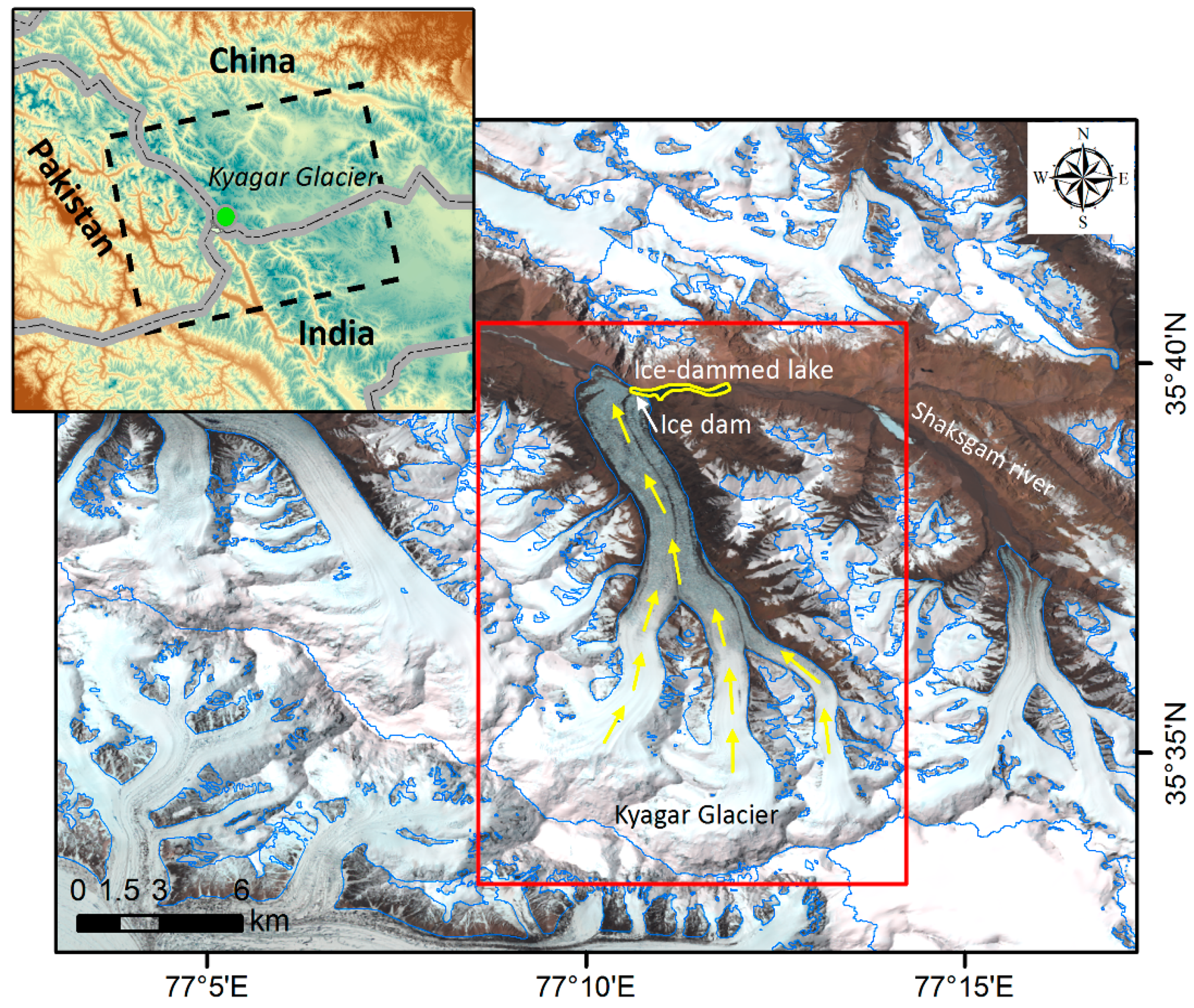
Our study area was the Kyagar Glacier, a large polythermal valley glacier located in the Chinese Karakoram Mountains. The glacier consists of three separate glacier tributaries 6–10 km in length that join into an 8 km-long glacier tongue, extending from 4800 m to almost 8000 m a.s.l. (Figure 1). The total area of the glacier is approximately 100 km2 based on the Randolph Glacier Inventory Version 5.0 dataset [23]. Kyagar Glacier has relatively gentle slopes, with an average surface slope of 2–3° over the tongue and 4–20° over the branches [24]. The Shaksgam Valley passes under the terminus of Kyagar Glacier. It was first recognized in the 1990s that this glacier sometimes dams the river in the Upper Shaksgam Valley and that there had been periods of advance or thickening in the late 1920s, 1970s, and 1990s [9]. During the past few years, the glacier terminus has advanced by several hundred meters and completely blocked the Shaksgam Valley, forming an ice-dammed lake. Kyagar Lake used to be one of the largest ice-dammed lakes in the world, with regular fill-up and drainage.
This region is largely controlled by westerly weather systems, with much of the precipitation occurring in the relatively warm season (May to September) and snow accumulating mainly in winter [25]. The average annual temperature is below 0 °C, indicating a cold climate. In recent studies, the observed mass balance values for the Karakoram glaciers have been near zero or slightly positive, which is in obvious contrast to the global trend of negative glacier mass balance in line with global warming [26,27]. However, these observations can possibly be explained by the regional precipitation increase in winter [25].
2.2. Data Sources
Recent advances in SAR technologies have provided much higher spatial resolution data from, for example, the TerraSAR-X and RADARSAT-2 sensors, data from which should be good options for the detection and analysis of glaciers and ice-dammed lakes [12,19,28]. However, Sentinel-1A data was chosen for use in this study because TerraSAR-X data works in the X-band (RADARSAT-2 and Sentinel-1 work in the C-band), which may result in incoherent data sets in the case of the monitoring of alpine glaciers. In addition, the free availability of Sentinel data means that it has a wide user community and has great potential to push forward remote sensing-based cryospheric research.
In order to evaluate how the dynamics of the Kyagar Glacier relate to the development of the impounded lake and to access its GLOF events of 10 August 2018, we used four pairs of interferometric wide swath (IW) mode Sentinel-1A images acquired during July to August of that year. These images had a fixed off-nadir look angle of 39.51°. Table 1 presents details of the Sentinel-1A data that were used, including their system parameters. The area covered by these images is indicated by a dashed rectangle in the inset in Figure 1. All the images were acquired in ascending orbit; the interval between the images in each pair was the shortest available—12 days. The range and azimuth pixel spacing of a standard IW mode Sentinel-1A image is ~5 m and 20 m, respectively [29,30]. Coherence and interferometric fringe maps derived from the SAR pairs were used for the characterization of typical cryospheric elements. Time series of SAR intensity data were used for visual assessment of lake formation and evolution. For the evaluation of climatic influences on the glacier surface area, meteorological variables including air temperature and precipitation amount were obtained from the ERA-Interim dataset produced by the European Centre for Medium-Range Weather Forecasts (ECMWF), recorded at the daily intervals during the whole year of 2018.
3. Methodology
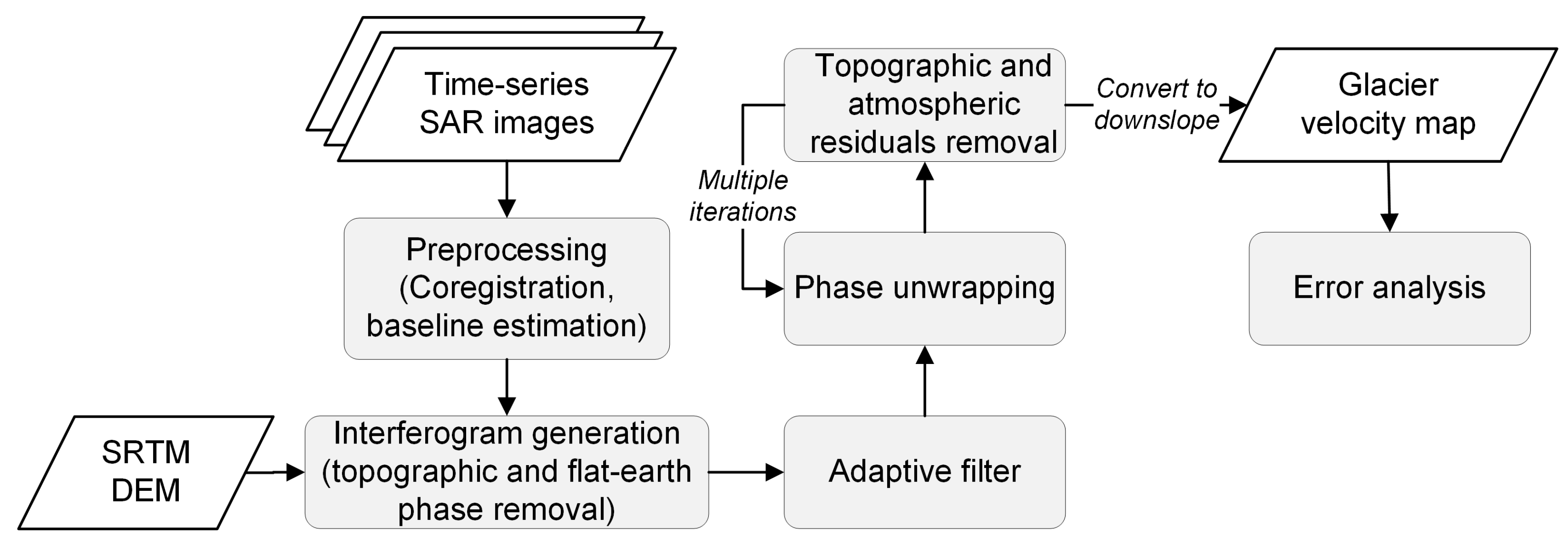
The methodology used for evaluating the spatio-temporal dynamics of the glacier surface and characterizing the ice-dammed lakes is given in Figure 2. Three steps were involved: preprocessing of SAR time series and generation of interferograms; converting the phase information to a glacier velocity map for the downslope; error analysis of the derived velocity value. More details of these steps are discussed in the sub-sections below.
3.1. Interferogram Processing
The preprocessing of SAR data and generation of interferograms were both implemented using the SARscape V5.2.1 software developed by the SARMAP SA Company. First, all the SAR data sets were geometrically coregistered to a reference image; perpendicular baselines between consecutive images were then derived so that the initial image coherence could be evaluated. Secondly, the standard InSAR processing procedures [31] were applied to the preprocessed image pairs to generate corresponding interferograms. Since the terrain in the study area is rugged, the topographic phase in the interferograms varies a lot and greatly influences the extracted displacement-dependent phase. Here, the 30-m Shuttle Radar Topography Mission (SRTM) Digital Elevation Model (DEM) was used to simulate the topography-related phase and then subtracted from the interferometric phase. We also used the fringe patterns over bedrock areas, where coherence is high and constant, to adjust the baseline so that the fringes over bedrock areas were flattened. In order to reduce the speckle noise and improve the signal-to-noise ratio of the interferograms, we applied an adaptive spectral filter [32] using a window size of 32 × 32 pixels. This interferometric phase was represented as a value in the range −π–π, with an unknown integer ambiguity of 2π. As the interferometric phase unwrapping is the most critical step in InSAR processing, the minimum cost flow (MCF) [33] method was used for this due to its superior ability to deal with sparse points. Finally, the residual topographic and atmospheric phase components were estimated by two-dimensional regression and removed after several iterations.
3.2. Glacier Surface Velocity Calculations
A surface velocity map () can be derived after converting the unwrapped phase to the magnitude of the displacement in the horizontal plane:
Here λ is the wavelength of the SAR signal, i.e., 5.6 cm in this study, and is the unwrapped interferometric phase due to glacier motion. refers to the interval between the acquisition times of the images in the pair.
However, these velocities in single-track interferograms are in the direction of the sensor line-of-sight (LOS). Additional steps are required to convert the LOS relative velocities to down-slope velocities along the glacier. Using the SRTM DEM slope information and the sensor−terrain geometry at the time of the image acquisitions [34], the horizontal flow velocity values () at the glacier surface can be calculated using the equation:
where is the radar incidence angle, and is the angle between the horizontal flow vector and the azimuth direction.
3.3. Error Analysis
The final InSAR velocity values may be influenced by many potential sources of error, which include the phase noise, noise related to atmospheric effects, the baseline error, the DEM error, and the phase unwrapping errors. Of these, the phase noise is caused by the incoherence between the images of the pair and generally contributes a relatively high component of about () cm/day to the noise in the velocity measurements [31]. Atmospheric noise is directly related to the local variations in atmospheric conditions over the study area and has a small effect on the glacier motion data of about ±0.5 cm/day. As for the baseline error, in the current study, due to the lack of ground control points (GCPs) in the field, the baseline estimation was based on the Precise Orbit Determination (POD) Precise Orbit Ephemerides files, which have a positioning accuracy better than 5 cm [35], and thus non-baseline refinement was not necessary. The DEM error is proportional to the baseline length and can be negligible in the case of sufficiently small baselines [34]. Finally, phase unwrapping from a starting point with non-zero velocity may introduce a small offset typically less than () cm/day to the derived velocity data [31]. Based on the above analyses, the total error from these sources in the calculated glacier surface velocities was approximately 2 cm/day and thus considerably smaller than the glacier movement signals, which are usually in the order of tens of centimeters.
4. Experimental Results
4.1. Analysis of Interferometric and Backscattering Properties
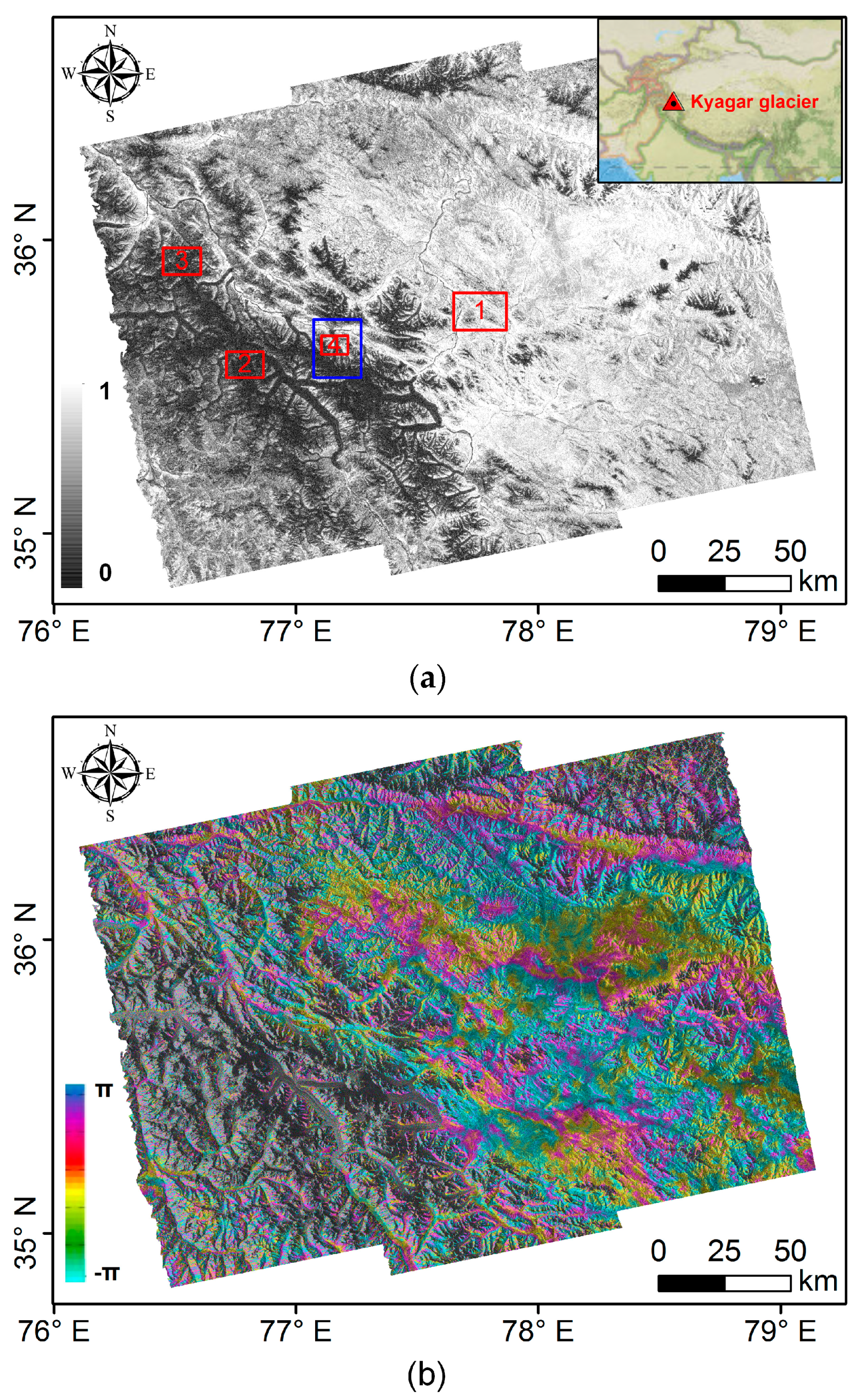
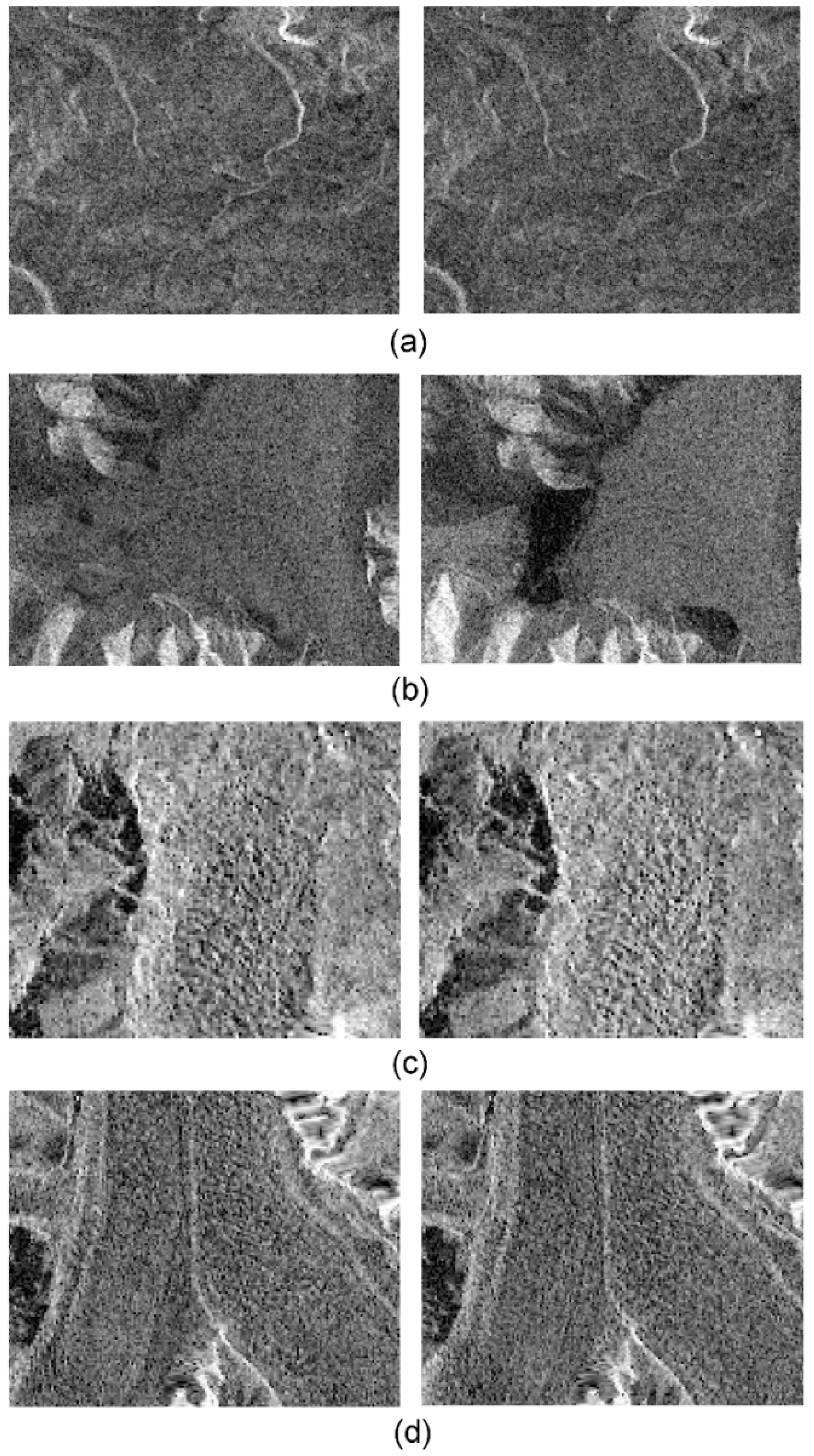
For the evaluation of the quality and reliability of DInSAR for the calculation of glacier surface velocities over such areas with surge-type glaciers, the coherence was estimated for change detection (Figure 3a). The region as a whole can be seen to have a high coherence of about 0.43, with a standard deviation of 0.17. This means that the coherence varies greatly across the region as the various cryospheric elements are characterized by distinct hydrological and geological processes. Four typical areas indicated in Figure 3a were selected for detailed comparison and analysis. In the no-motion area (e.g., bedrock), the homogeneous intensity implies that there was little movement during the time period, resulting in a high level of coherence (Figure 4a). A characteristic of the surface of ice-dammed lakes is a large amount of floating ice. Therefore, the physical properties of the ice-dammed lake may change over time in a natural manner [36]. Lake ice is a typical example of this kind of inherent change that occurs as a result of climate conditions. In particular, it should be noted that serious loss of coherence can be related to the ice thickness, which makes the characteristics of radar responses from glacial lakes much more complicated [37,38]. The ice-free lake can be easily identified in the image acquired on 18 August due to the low returns from the water surface (Figure 4b). However, the presence of ice on the lake may introduce multiple backscattering between the ice and water, and thus increase the return power, making the lake almost indistinguishable from the background. Glacier motion is frequently observed in these glaciated areas. Although a coherent interferometric phase cannot always be obtained for a glacier, offset motion is more likely to result in coherent data [18,39]. Therefore, this motion type was analyzed for two different areas shown in Figure 4c,d. Debris-covered glaciers, which can appear to be normal terrain with ponds and vegetation, produce incoherent values (Figure 4c). This can produce uncertainty in the estimates of velocity in areas with this type of glacial feature. However, for moving glaciers that are free of debris, the coherent phase obtained over a small time-scale allows complete measurement of the surface flow (Figure 4d). The analysis of four experimental results shows that fairly accurate estimates of glacier movement can be made for the study area using the InSAR-based technique; it should also be remembered that each estimate is directly related to the characteristics of the target objects.
4.2. Time Series of Velocity Estimates for the Whole Glacier
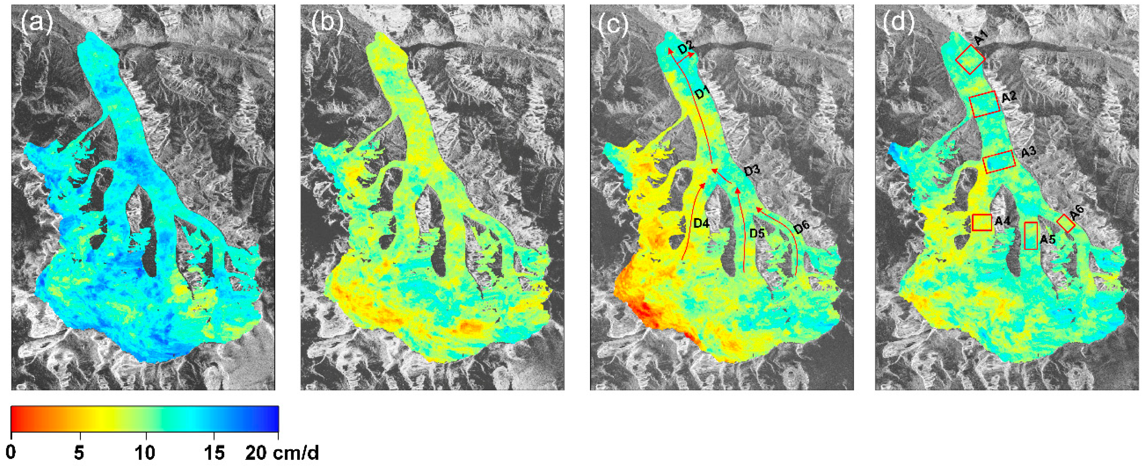
The detection of the surface velocity field over a whole glacier and velocity changes over time can be continuously carried out using InSAR-based technology. These velocity fields were calculated for consecutive 12-day periods (Figure 5). The surge acceleration appears to be significant at the beginning of July, with a maximum velocity of around 20 cm/day over 12 days (Figure 5a). The maximum instantaneous velocity is higher than the values averaged over 12-day periods. After the surge peak that started on 1 July, there was a rapid deceleration, causing the maximum velocities to drop to about 13 cm/day by 25 July (Figure 5b). This abrupt slow-down coincided with the pre-drainage of the subglacial water. After that, it was followed by a new phase of acceleration, which continued from 25 July to 6 August, with the velocity reaching almost 18 cm/day on 18 August (Figure 5c,d), slightly faster than the peak velocity in the previous phase. Although there was a slight acceleration after 25 July, velocities were still significantly below the surge phase, remaining below 15 cm/day over the tongue. Moreover, it was noticed that, after the drainage of the lake on 10 August, the flow velocities in the tributary did not sharply decrease because drainage mass loss needed to be replenished by the fast flow of ices [19].
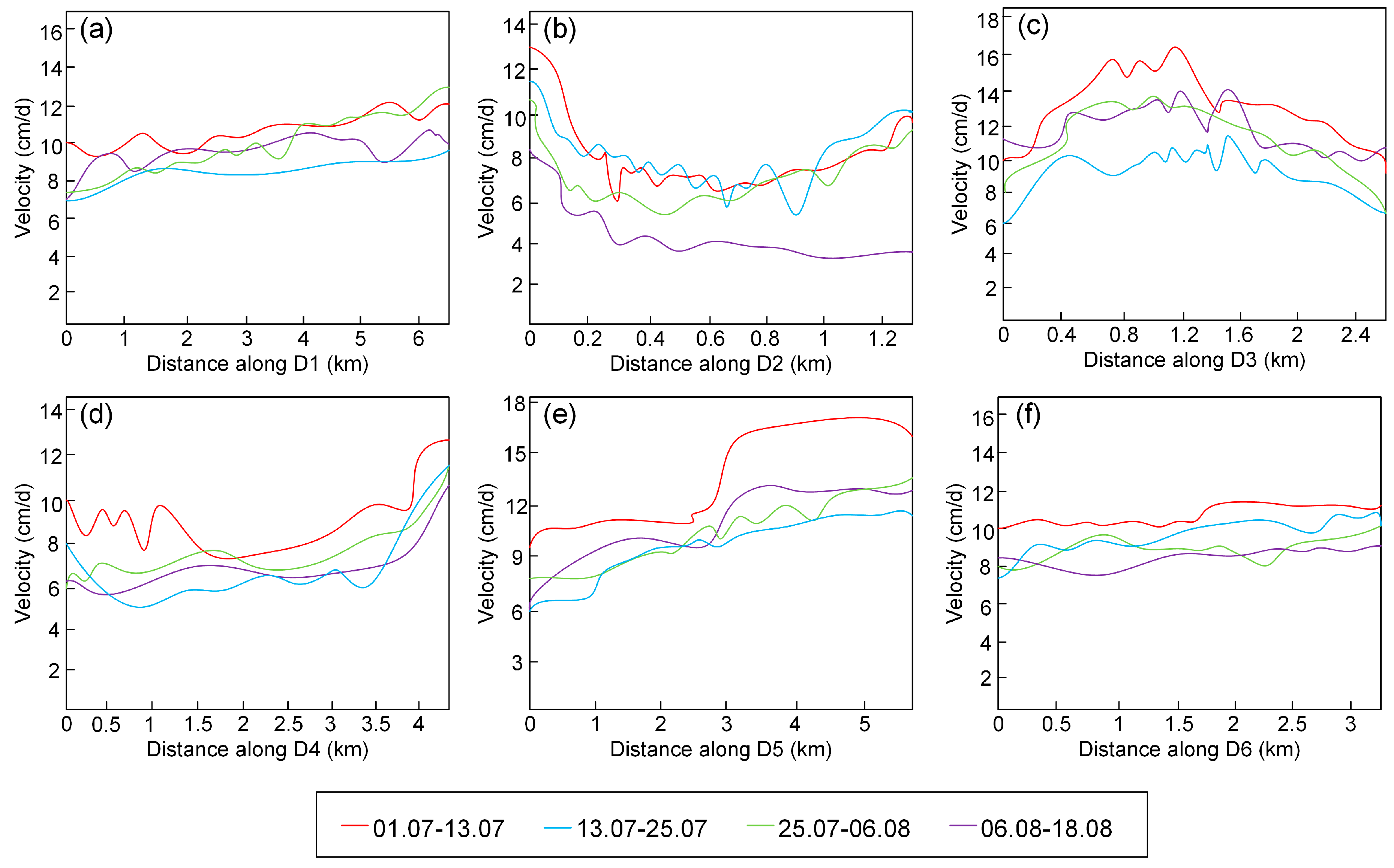
We also extracted the velocities along six profiles (indicated in Figure 5c) and within six regions (indicated in Figure 5d) over the entire study period so that quantitative comparisons could be made (Figure 6 and Table 2). The spatial variations in the glacier velocities were continuous, which is consistent with the basic features of glacier movement [39]. The peak of glacier motion also occurred between 1 July and 13 July. During the surge development, a clear movement occurred that was the greatest over the main axis along the glacier tongue (profiles D1, D3, and D5) and which had a maximum velocity of about 17 cm/day in early July (Figure 6a,c,e). There was a substantial change at the front of the ice dam before and after the lake outburst (Figure 6b), with a gradual deceleration towards the glacial lake. Except for the trunk glacier (Figure 6e), most of the lateral tributary had velocities between 6 cm/day and 11 cm/day during the observation periods (Figure 6d,f). The western side of the tributary showed larger fluctuations than the relatively steady velocities observed on the eastern side.
Table 2 shows the average values of the motion estimates for the key regions. Apart from the fast movement observed in the early study period, from 13 July to 18 August, the glacier tongue (A1−A3) velocity increased: the increasing gradient was greater in the upper reaches of region A3 with a continuous increase by 57.5% from 7.3 cm/day to 11.5 cm/day. The downward velocity increased by only 13.0% (0.9 cm/day) in region A1, glacier terminus that shows large variations during this time, and by 26.9% (2.4 cm/day) in region A2. The velocity across the tributary above the confluence (A4−A6) showed different trends. In region A5, the velocity increased by 16.2% (1.7 cm/day). However, in regions A4 and A6 it decreased by 11.8% (0.9 cm/day) and 10.2% (1.0 cm/day), respectively.
These results and the associated analysis demonstrate that an obvious acceleration in the motion of Kyagar Glacier can be observed in the pre-drainage phase of its glacial lake. Rapid deceleration first became evident between 13 July and 25 July; after that, the velocities continued increasing steadily until the lake outburst event that occurred on 10 August. There was a much larger increase in the velocity of the upper part of the glacier tongue prior to the lake outburst.
4.3. Lake Development and Drainage
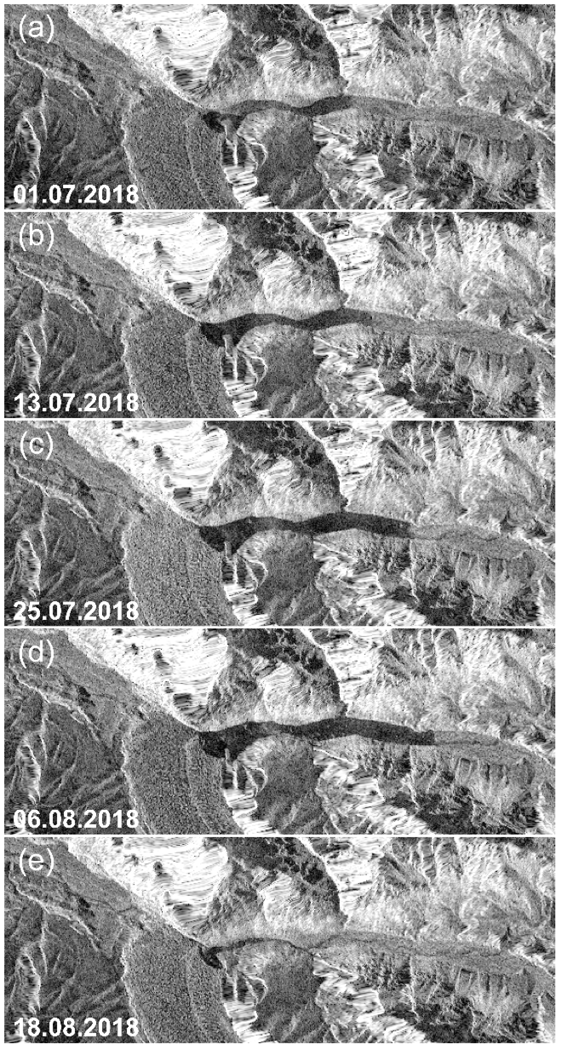
Rapidly developing glacial lakes are generally identified as potentially dangerous glacial lakes. These lakes are more vulnerable to GLOFs than other glacial lakes, and deserve more attention in term of continuous monitoring. Time series of radar backscattering images from Sentinel-1A for the Kyagar Glacier show that this glacial lake formed in the river basin upstream of the glacier terminus (Figure 7). During July and August 2018, the lake appeared to fill faster in line with the onset of summer ice melting. Compared with 13 July, by 25 July the water surface had risen significantly. This is because the high-temperature water had eroded the base of the ice dam and part of the ice dam finally loosened and collapsed. The water level of the lake continued to rise on 6 August as the broken and floating ice melted until the lake reached an estimated area of 2.4 km2 before draining. With the increasing lake area and thus the increasing water pressure on the ice dam, the probability of dam failure increased, which finally led to the sudden drainage of the lake on 10 August 2018. It can be clearly seen that the outburst events for this large ice-dammed lake are most probably characterized by the process of dam collapse or overtopping, rather than through subglacial drainage [9]. On 18 August, the lake area had shrunk considerably to form a new space and the lower reaches of the river had widened. Due to the glacier surge movement and abundant glacial meltwater, new ice-dammed lakes will develop and suddenly breach periodically [40].
4.4. Glaciological Observations
Through the evolution of a subglacial drainage system of Kyagar Glacier towards the end of August, it can be observed rapid acceleration at the early stage of July, which can be explained by the much more input of meltwater and subsequently the increased water pressure for an inefficient subglacial drainage system. This subglacial drainage system seems to be present during the whole observation period. After reaching maximum velocities, the deceleration indicates there was a transient decrease in subglacial water pressure that results from the decreased input meltwater and possible subglacial drainage. Through August, as meltwater continued to input, another acceleration reflects that subglacial water pressure is increasing during this time. The observed lake formation is clear evidence for the drainage of en- or sub-glacially stored water [36]. The drainage of subglacial water appeared to end in mid-August with the growth of the ice-dammed lake. When the lake outburst event happened, most subglacial water was drained, and subglacial drainage channels perhaps closed towards the end of the summer. This rapid evolution of the drainage system was caused by the boundary condition change, namely the sudden decrease in water pressure as the lake at the glacier terminus drained [41].
4.5. Meteorological Observations
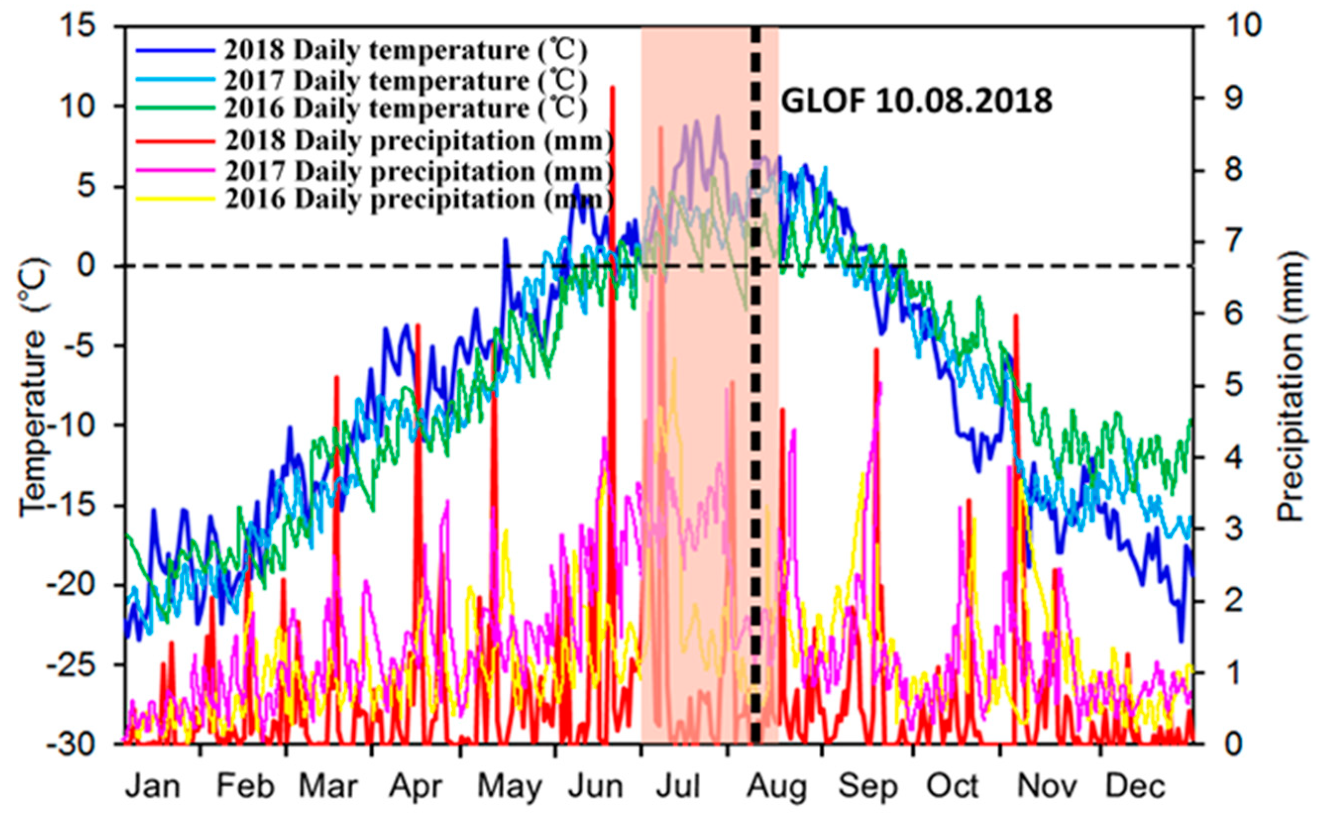
The dynamics of recent glacier movements and ice-dammed lake outbursts have definite strong connections to climate change. We used daily air temperatures and precipitation data from the ECMWF numerical weather prediction model for operational analysis (Figure 8). From 2016 to 2018, air temperature exhibited a similar trend. A constant increase in air temperature began in March, with the temperature reaching its peak values in July and August, at a time when temperatures were consistently well above 0 °C. Meanwhile, it was surprising to find that precipitation was higher in June and July of 2018 compared with previous years. The relatively higher and sustained increase in air temperature in 2018, together with a simultaneous increase in precipitation, intensified the ablation process on the glacier surface. The calculated total melt is about 3972.8 mm during the ablation season [42], this high total melt further confirms the accelerating melting of Kyagar Glacier. Before the GLOF events, an apparent peak in the air temperature and extremely high precipitation which last for several days can be observed. A large amount of rainfall and meltwater increased the pressure at the glacier base, leading to a reduction in frictional strength and finally to an increase in the basal sliding of the glacier [19,43]. The contribution of precipitation and ice-melt to the discharge of the Shaksgam River is expected to have large variations in a short time. Coincided with melt seasons, the discharge of Shaksgam River increased significantly, which intensify the en- and sub-glacial water drainage, and finally influence ice dam breaching. Overall, we can conclude that glacier motion changes should be interpreted as a consequence of this rather warm period and high precipitation just before the lake outburst, and the behavior of the ice dam was also affected by the Shaksgam River discharge changes.
5. Discussion
5.1. Interactions of Kyagar Glacier with the Glacial Lake and Its Surge Mechanism
We investigated the interactions of Kyagar Glacier with the ice-dammed lake using the DInSAR technique to derive a time-series of glacier motion. The Kyagar Glacier has experienced a rapid surge termination before the 2018 GLOF. During the active surge phase, the glacier surface displacement maps demonstrate that the glacier typically experiences dramatic lengthening or thickening at the terminus with potentially hazardous consequences (Figure 5), such as the formation of an ice-dammed lake. The lake area quickly expanded during the summer because of significant snow/ice ablation as a result of most of the days being above 0 °C (Figure 7). This is because there is a well-established relationship between positive degree-day totals and snow/ice melting [44,45,46,47]. Another source of the glacial lake is the flowing water from the Shaksgam River, which may also increase the lake water level. The surge process enabled much more ice from the glacier tongue to extend into the lake [48]. With declined velocity towards the end of the glacier tongue (Figure 6b), the morphology of the glacier tongue longitudinal profile has changed. At the ice-flow direction, there are radial and transverse crevasses due to the completely detached and separated ice blocks, which may transform into ice bungles during the surge. Under the glacier, the depth and width of these crevasses also increase. Specifically, due to the thermal erosion, the increase in lake volume during the ablation season increased contact ice ablation and the risk of a dam collapse. Ice calving then began when the lake water gradually lifted the ice dam, causing greater loss of glacier mass than that due to normal ablation. To try to replenish the front mass loss, during the post-outburst phases, the tributary accelerated and therefore the mass loss from the glacier further intensified.
A surge mechanism is usually defined as a switch in basal thermal conditions, namely, when glacier basal conditions switch from cold to temperate, a surging occurs. As a typical polythermal glacier, Kyagar Glacier has already been temperate at the base [49,50], and its surge can be explained by a hydrological switch mechanism. When the subglacial drainage system is inefficient, the pressure from subglacial water increases, and accelerates the rapid sliding of the base, a surge will occur [51,52]. Therefore, rapid basal sliding during the glacier surge is seemingly controlled by high water pressure, which is caused by the surface water entering the inefficient subglacial drainage system or unstable subglacial till. The various phases of the glacier surge were all triggered by a basal motion mechanism [48]. The spatial distribution and temporal changes in velocity over the Kyagar Glacier provide additional information about the nature of surge. It is obvious that the tongue of the glacier primarily experienced surging—this observation is supported by the risen velocity along the glacier tongue during the data acquisition period (Table 2). The surge phenomenon was mainly confined to the flatter, lower part of the glacier as has already been observed for a number of Karakoram glacier surges [53,54].
5.2. Lake Outburst Mechanism
Long-term observations confirm that outbursts from this ice-dammed lake are periodic [9,11]. Based on our findings and previous results, we suggest that these periodic outbursts are the result of the combined effects of ice dam collapse and overtopping. The subglacial channels provide a weaker, preferential pathway for lake drainage, and thus lead to an earlier outburst. In this case, the obvious deceleration at the end of July 2018, occurring in association with the subglacial drainage, is an early warning signal of the lake outburst (Figure 5). It seems that the opening of subglacial channels beneath the terminus before the lake outburst reduced the subglacial water pressure and, hence, the velocity decreased beneath the entire glacier tongue within 12 days. In certain circumstances, the cracking of the englacial cavity and the lifting of the ice dam play key roles in the acceleration of glacial lake outburst floods. However, the lifting of the ice dam is a gradual process and the excessive englacial pressure from the volume of lake water, rather than the floating of the ice dam, appears to control this particular water drainage system.
6. Conclusions
The recent surge cycle of Kyagar Glacier, in the Chinese Karakoram, caused the formation of an ice-dammed lake and subsequent GLOFs on 10 August 2018, but the role of this glacier surge in GLOF formation was previously unrecognized. Besides, in the glacial environment, due to snowfall, melting, and ice flows at a variety of spatial and temporal scales, glacier monitoring exhibits complex spatial and temporal dynamics. The harsh climate conditions during the lake outburst event make cryospheric studies even more challenging. All these complex characteristics mean that special techniques and new satellite sensors with wider applications, high data availability, and spatio-temporal resolution, such as Sentinel-1, are required for the characterization of Kyagar Glacier and the associated lake outburst floods.
In this study, it has been demonstrated that a time-series of glacier motion based on the InSAR technique is effective for assessing the dynamics of a mountain glacial system and the interactions between the glacier and the glacial lake. Velocity fields show the maximum velocity reached in early July, followed by a sudden deceleration from the middle of July to August. During this time the velocity changed in a consistent way but slightly increased overall. The dramatic acceleration of the glacier also coincided with the melt season and high rainfall, and the surge continued following the 2018 GLOF. Combing these velocity data with detailed meteorological information indicates that the glacial lake is sensitive to the movement of the glacier and also local climate variations. Ice dam collapse or water overtopping were direct factors leading to this GLOF, while subglacial water under a large part of the glacier tongue also occurred during the lake outburst event. Considering the repeated occurrences of outburst flood hazards, this ice-dammed lake formation and its evolution should be carefully monitored using advanced remote sensing techniques for the warning of large GLOFs in the future.
Author Contributions
M.Z., F.C., and B.T. contributed the main idea and designed the experiments; M.Z. and D.L. performed the experiments; A.Y. analyzed the SAR data; M.Z. wrote the manuscript, which was then improved by the contribution of all the co-authors. All authors have read and agreed to the published version of the manuscript.
Funding
This research was funded by the National Key R&D Program of China (Grant No.2017YFE0100800), the International Partnership Program of the Chinese Academy of Sciences (Grant No.131551KYSB20160002/131211KYSB20170046), and the National Natural Science Foundation of China (41871345).
Conflicts of Interest
The authors declare no conflict of interest.
References
- Richardson, S.D.; Reynolds, J.M. An overview of glacial hazards in the Himalayas. Quat. Int. 2000, 65, 31–47. [Google Scholar] [CrossRef]
- Huggel, C.; Kääb, A.; Haeberli, W.; Teysseire, P.; Paul, F. Remote sensing based assessment of hazards from glacier lake outbursts: A case study in the Swiss Alps. Can. Geotech. J. 2002, 39, 316–330. [Google Scholar] [CrossRef] [Green Version]
- Weckwerth, P.; Wysota, W.; Piotrowski, J.A.; Adamczyk, A.; Krawiec, A.; Dąbrowski, M. Late weichselian glacier outburst floods in North-eastern Poland: Landform evidence and palaeohydraulic significance. Earth-Sci. Rev. 2019, 194, 216–233. [Google Scholar] [CrossRef]
- Meinsen, J.; Winsemann, J.; Weitkamp, A.; Landmeyer, N.; Lenz, A.; Dölling, M. Middle pleistocene (saalian) lake outburst floods in the münsterland embayment (NW Germany): Impacts and magnitudes. Quat. Sci. Rev. 2011, 30, 2597–2625. [Google Scholar] [CrossRef]
- Westoby, M.J.; Glasser, N.F.; Brasington, J.; Hambrey, M.J.; Quincey, D.J.; Reynolds, J.M. Modelling outburst floods from moraine-dammed glacial lakes. Earth-Sci. Rev. 2014, 134, 137–159. [Google Scholar] [CrossRef] [Green Version]
- Dan, H.S.; Clague, J.J. The sedimentology and geomorphology of rock avalanche deposits on glaciers. Sedimentology 2011, 58, 1762–1783. [Google Scholar]
- Cook, K.L.; Andermann, C.; Gimbert, F.; Adhikari, B.R.; Hovius, N. Glacial lake outburst floods as drivers of fluvial erosion in the Himalaya. Science 2018, 362, 53–57. [Google Scholar] [CrossRef] [Green Version]
- Krabbendam, M.; Glasser, N.F. Glacial erosion and bedrock properties in NW Scotland: Abrasion and plucking, hardness and joint spacing. Geomorphology 2011, 130, 374–383. [Google Scholar] [CrossRef] [Green Version]
- Hewitt, K.; Liu, J.S. Ice-dammed lakes and outburst floods, Karakoram Himalaya: Historical perspectives on emerging threats. Phys. Geogr. 2010, 31, 528–551. [Google Scholar] [CrossRef]
- Emmer, A. Glofs in the wos: Bibliometrics, geographies and global trends of research on glacial lake outburst floods (web of science, 1979–2016). Nat. Hazards Earth Syst. Sci. 2018, 18, 813–827. [Google Scholar] [CrossRef] [Green Version]
- Haemmig, C.; Huss, M.; Keusen, H.; Hess, J.; Wegmüller, U.; Ao, Z.; Kulubayi, W. Hazard assessment of glacial lake outburst floods from Kyagar Glacier, Karakoram Mountains, P.R. China. Ann. Glaciol. 2014, 55, 34–44. [Google Scholar] [CrossRef] [Green Version]
- Round, V.; Leinss, S.; Huss, M.; Haemmig, C.; Hajnsek, I. Surge dynamics and lake outbursts of Kyagar Glacier, Karakoram. Cryosphere 2017, 11, 723–739. [Google Scholar] [CrossRef] [Green Version]
- Liu, J.J.; Cheng, Z.L.; Su, P.C. The relationship between air temperature fluctuation and glacial lake outburst floods in Tibet, China. Quat. Int. 2014, 321, 78–87. [Google Scholar] [CrossRef]
- Hogas, F.; Longva, O. Mega deposits and erosive features related to the glacial lake nedre glomsjø outburst flood, Southeastern Norway. Quat. Sci. Rev. 2016, 151, 273–291. [Google Scholar] [CrossRef]
- Erten, E.; Reigber, A.; Hellwich, O.; Prats, P. Glacier velocity monitoring by maximum likelihood texture tracking. IEEE Trans. Geosci. Remote Sens. 2009, 47, 394–405. [Google Scholar] [CrossRef] [Green Version]
- Tian, B.; Li, Z.; Tang, P.; Zou, P.; Zhang, M.; Niu, F. Use of intensity and coherence of x-band sar data to map thermokarst lakes on the Northern Tibetan Plateau. IEEE J. Sel. Top. Appl. Earth Obs. Remote Sens. 2016, 9, 3164–3176. [Google Scholar] [CrossRef]
- Xia, G.S.; Liu, G.; Yang, W.; Zhang, L. Meaningful object segmentation from SAR images via a multiscale nonlocal active contour model. IEEE Trans. Geosci. Remote Sens. 2015, 54, 1860–1873. [Google Scholar] [CrossRef] [Green Version]
- Kumar, V.; Venkataraman, G.; Høgda, K.A.; Larsen, Y. Estimation and validation of glacier surface motion in the Northwestern Himalayas using high-resolution SAR intensity tracking. Int. J. Remote Sens. 2013, 34, 5518–5529. [Google Scholar] [CrossRef]
- Jia, L.; Li, Z.W.; Wu, L.X.; Bing, X.; Hu, J.; Zhou, Y.S.; Miao, Z.L. Deriving a time series of 3d glacier motion to investigate interactions of a large mountain glacial system with its glacial lake: Use of synthetic aperture radar pixel offset-small baseline subset technique. J. Hydrol. 2018, 559, 596–608. [Google Scholar]
- Quincey, D.J.; Richardson, S.D.; Luckman, A.; Lucas, R.M.; Reynolds, J.M.; Hambrey, M.J.; Glasser, N.F. Early recognition of glacial lake hazards in the Himalaya using remote sensing datasets. Glob. Planet. Chang. 2007, 56, 137–152. [Google Scholar] [CrossRef]
- Capps, D.M.; Rabus, B.; Clague, J.J.; Shugar, D.H. Identification and characterization of alpine subglacial lakes using interferometric synthetic aperture radar (insar): Brady Glacier, Alaska, USA. J. Glaciol. 2010, 56, 861–870. [Google Scholar] [CrossRef] [Green Version]
- Sánchez-Gámez, P.; Navarro, F. Glacier surface velocity retrieval using d-insar and offset tracking techniques applied to ascending and descending passes of sentinel-1 data for southern ellesmere ice caps, Canadian Arctic. Remote Sens. 2017, 9, 442. [Google Scholar] [CrossRef] [Green Version]
- Arendt, A.; Bolch, T.; Cogley, J.; Gardner, A.; Hagen, J.; Hock, R.; Kaser, G.; Pfeffer, W.; Moholdt, G.; Paul, F. Randolph Glacier Inventory—A Dataset of Global Glacier Outlines: Version 5.0; GLIMS Technical Report; Digital Media: Boulder, CO, USA, 2015. [Google Scholar]
- Searle, M.P.; Phillips, R.J. Relationships between right-lateral shear along the Karakoram fault and metamorphism, magmatism, exhumation and uplift: Evidence from the k2-gasherbrum-pangong ranges, North Pakistan and Ladakh. J. Geol. Soc. 2007, 164, 439–450. [Google Scholar] [CrossRef]
- Kapnick, S.B.; Delworth, T.L.; Ashfaq, M.; Malyshev, S.; Milly, P.C.D. Snowfall less sensitive to warming in Karakoram than in Himalayas due to a unique seasonal cycle. Nat. Geosci. 2014, 7, 834–840. [Google Scholar] [CrossRef]
- Gardner, A.S.; Moholdt, G.; Cogley, J.G.; Wouters, B.; Arendt, A.A.; Wahr, J.; Berthier, E.; Hock, R.; Pfeffer, W.T.; Kaser, G. A reconciled estimate of glacier contributions to sea level rise: 2003 to 2009. Science 2013, 340, 852–857. [Google Scholar] [CrossRef] [PubMed] [Green Version]
- Bhambri, R.; Bolch, T.; Kawishwar, P.; Dobhal, D.P.; Pratap, B. Heterogeneity in glacier response in the upper shyok valley, Northeast Karakoram. Cryosphere 2013, 7, 1385–1398. [Google Scholar] [CrossRef] [Green Version]
- Strozzi, T.; Wiesmann, A.; Kaab, A.; Joshi, S. Glacial lake mapping with very high resolution satellite sar data. Nat. Hazards Earth Syst. Sci. Discuss. 2012, 12, 2487–2498. [Google Scholar] [CrossRef] [Green Version]
- Nguyen, D.B.; Gruber, A.; Wagner, W. Mapping rice extent and cropping scheme in the Mekong Delta using sentinel-1a data. Remote Sens. Lett. 2016, 7, 1209–1218. [Google Scholar] [CrossRef]
- Zinno, I.; Casu, F.; Luca, C.D.; Elefante, S.; Lanari, R.; Manunta, M. A cloud computing solution for the efficient implementation of the p-sbas dinsar approach. IEEE J. Sel. Top. Appl. Earth Obs. Remote Sens. 2017, 10, 802–817. [Google Scholar] [CrossRef]
- Fatland, D.R.; Lingle, C.S. Analysis of the 1993–1995 bering glacier (Alaska) surge using differential sar interferometry. J. Glaciol. 1998, 44, 532–546. [Google Scholar] [CrossRef] [Green Version]
- Goldstein, R.M.; Werner, C.L. Radar interferogram filtering for geophysical applications. Geophys. Res. Lett. 1998, 25, 4035–4038. [Google Scholar] [CrossRef] [Green Version]
- Costantini, M. A novel phase unwrapping method based on network programming. Geosci. Remote Sens. IEEE Trans. 1998, 36, 813–821. [Google Scholar] [CrossRef]
- Goldstein, R.M.; Engelhardt, H.; Kamb, B.; Frolich, R.M. Satellite radar interferometry for monitoring ice sheet motion: Application to an Antarctic ice stream. Science 1993, 262, 1525–1530. [Google Scholar] [CrossRef] [PubMed]
- Peter, H.; Jäggi, A.; Fernández, J.; Escobar, D.; Ayuga, F.; Arnold, D.; Wermuth, M.; Hackel, S.; Otten, M.; Simons, W. Sentinel-1a-first precise orbit determination results. Adv. Space Res. 2017, 60, 879–892. [Google Scholar] [CrossRef]
- Xie, Z.; Zhang, S.; Ding, Y.; Liu, S.; Shangguan, D. Index for hazard of glacier lake outburst flood of Lake Merzbacher by satellite-based monitoring of lake area and ice cover. Glob. Planet. Chang. 2012, 107, 229–237. [Google Scholar] [CrossRef]
- Dammert, P.B.G.; Lepparanta, M.; Askne, J. Sar interferometry over baltic sea ice. Int. J. Remote Sens. 1998, 19, 3019–3037. [Google Scholar] [CrossRef]
- Arp, C.D.; Jones, B.M.; Urban, F.E.; Grosse, G. Hydrogeomorphic processes of thermokarst lakes with grounded-ice and floating-ice regimes on the Arctic coastal plain, Alaska. Hydrol. Process. 2011, 25, 2422–2438. [Google Scholar] [CrossRef]
- Neelmeijer, J.; Motagh, M.; Wetzel, H.U. Estimating spatial and temporal variability in surface kinematics of the Inylchek Glacier, Central Asia, using terrasar–x data. Remote Sens. 2014, 6, 9239–9259. [Google Scholar] [CrossRef] [Green Version]
- Glazirin, G.E. A century of investigations on outbursts of the ice-dammed Lake Merzbacher (Central Tien Shan). Austrian J. Earth Sci. 2010, 103, 171–179. [Google Scholar]
- Thompson, S.S.; Benn, D.I.; Dennis, K.; Luckman, A. A rapidly growing moraine-dammed glacial lake on Ngozumpa Glacier, Nepal. Geomorphology 2012, 145, 1–11. [Google Scholar] [CrossRef]
- Braun, L.N.; Grabs, W.; Rana, B. Application of a conceptual precipitation-runoff model in the Langtang Khola Basin, Nepal Himalaya. Snow and glacier hydrology. IAHS Publ 1993, 218, 221–237. [Google Scholar]
- Helgi, B. Hydrological characteristics of the drainage system beneath a surging glacier. Nature 1998, 395, 771–774. [Google Scholar]
- Braithwaite, R.J. Positive degree-day factors for ablation on the Greenland ice sheet studied by energy-balance modelling. J. Glaciol. 1995, 41, 153–160. [Google Scholar] [CrossRef] [Green Version]
- Hughes, P.D.; Braithwaite, R.J. Application of a degree-day model to reconstruct pleistocene glacial climates. Quat. Res. 2008, 69, 110–116. [Google Scholar] [CrossRef]
- Hughes, D.P. Twenty-first century glaciers and climate in the Prokletije Mountains, Albania. Arct. Antarct. Alp. Res. 2009, 41, 455–459. [Google Scholar] [CrossRef] [Green Version]
- Hughes, P.D. Response of a Montenegro glacier to extreme summer heatwaves in 2003 and 2007. Geogr. Ann. 2008, 90, 259–267. [Google Scholar] [CrossRef]
- Sobota, I.; Weckwerth, P.; Nowak, M. Surge dynamics of Aavatsmarkbreen, Svalbard, inferred from the geomorphological record. Boreas 2016, 45, 360–376. [Google Scholar] [CrossRef]
- Sevestre, H.; Benn, D.I. Climatic and geometric controls on the global distribution of surge-type glaciers: Implications for a unifying model of surging. J. Glaciol. 2015, 61, 646–662. [Google Scholar] [CrossRef] [Green Version]
- Lyså, A.; Larsen, E.A.; Høgaas, F.; Jensen, M.A.; Szczuciński, W. A temporary glacier-surge ice-dammed lake, Braganzavågen, Svalbard. Boreas 2018, 47, 837–854. [Google Scholar] [CrossRef] [Green Version]
- Sobota, I.; Nowak, M.; Weckwerth, P. Long-term changes of glaciers in North-western Spitsbergen. Glob. Planet. Chang. 2016, 144, 182–197. [Google Scholar] [CrossRef]
- Lovell, A.M.; Carr, J.R.; Stokes, C.R. Topographic controls on the surging behaviour of Sabche Glacier, Nepal (1967 to 2017). Remote Sens. Environ. 2018, 210, 434–443. [Google Scholar] [CrossRef] [Green Version]
- Mayer, C.; Fowler, A.C.; Lambrecht, A.; Scharrer, K. A surge of north Gasherbrum Glacier, Karakoram, China. J. Glaciol. 2011, 57, 904–916. [Google Scholar] [CrossRef] [Green Version]
- Quincey, D.J.; Glasser, N.F.; Cook, S.J.; Luckman, A. Heterogeneity in Karakoram glacier surges. J. Geophys. Res. Earth Surf. 2015, 120, 1288–1300. [Google Scholar] [CrossRef] [Green Version]
Figure 1.
Study area (Shaksgam Valley). Blue curves: outlines of glaciers; yellow curve: outline of the ice-dammed lake; yellow arrows: approximate directions of horizontal glacier flow; dashed rectangle in inset: frame of Sentinel-1A images; red rectangle in the main panel: area shown in Figure 5.
Figure 1.
Study area (Shaksgam Valley). Blue curves: outlines of glaciers; yellow curve: outline of the ice-dammed lake; yellow arrows: approximate directions of horizontal glacier flow; dashed rectangle in inset: frame of Sentinel-1A images; red rectangle in the main panel: area shown in Figure 5.

Figure 2.
InSAR-based processing steps for the calculation of glacier surface velocities.

Figure 3.
(a) Differential synthetic aperture radar (SAR) interferometry (DInSAR) coherence image, derived from Sentinel-1A SAR data acquired on 6 August 2018 and 18 August 2018. The numbered areas marked in the coherence image are test samples shown in Figure 4; the blue rectangle indicates the location of Kyagar Glacier. (b) Interferometric phase map of the test area. The background is from the intensity image. The color scale gives the DInSAR phase.

Figure 4.
Intensity images of four test areas: (a) no-motion area; (b) small glacial lake with ice on the surface. The ice thickness complicates the radar response characteristics. The lake can easily be identified in the second image based on the low return whereas it is almost invisible in the first image due to the high return; (c) typical glacier surface with debris cover; (d) part of the glacier that has coherent characteristics. The first and second column shows the intensity images obtained on 6 August 2018 and 18 August 2018, respectively.

Figure 5.
Time series of glacier flow velocities during four periods: (a) 1 July 2018−13 July 2018; (b) 13 July 2018−25 July 2018; (c) 25 July 2018−6 August 2018; (d) 6 August 2018−18 August 2018. The background image is from Sentinel-1A intensity data. The red curves (D1−D6) in (c) mark the profiles shown in Figure 6, and the red rectangles (A1−A6) in (d) mark the areas shown in Table 2.

Figure 6.
Velocities along the six profiles (D1−D6) indicated in Figure 5c.
Figure 6.
Velocities along the six profiles (D1−D6) indicated in Figure 5c.

Figure 7.
Radar backscattering images of the glacier terminus showing the lake dynamics before drainage (a−d) and (e) after the drainage.
Figure 7.
Radar backscattering images of the glacier terminus showing the lake dynamics before drainage (a−d) and (e) after the drainage.

Figure 8.
Daily 2 m temperature and total precipitation values for 2016–2018 for the Kyagar Glacier area taken from the European Centre for Medium-Range Weather Forecasts (ECMWF) model. The dashed line marks the glacial lake outburst flood (GLOF) in 2018 and the shaded rectangle marks the time frame covered by the observational data in this study.


Table 1.
List of temporal pairs of Sentinel-1A Interferometric Wide Swath (IW) mode data used for glacier movement estimation.
Table 1.
List of temporal pairs of Sentinel-1A Interferometric Wide Swath (IW) mode data used for glacier movement estimation.
| No. | Temporal Pairs(dd/mm/yyyy) | Temporal Baseline | Perpendicular Baseline (m) | System Parameters |
|---|---|---|---|---|
| 1 | 01/07/2018 and 13/07/2018 | 12 days | 8.197 | Pass direction: Ascending Range pixel spacing: 5 m Azimuth pixel spacing: 20 m Off-nadir angle: 39.51° |
| 2 | 13/07/2018 and 25/07/2018 | 12 days | 43.773 | |
| 3 | 25/07/2018 and 06/08/2018 | 12 days | 39.391 | |
| 4 | 06/08/2018 and 18/08/2018 | 12 days | 54.600 |
Table 2.
Average velocities for the six regions A1−A6, indicated in Figure 5d, during four time periods.
Table 2.
Average velocities for the six regions A1−A6, indicated in Figure 5d, during four time periods.
| Region | Area (km2) | Average Velocity (cm/day) | |||
|---|---|---|---|---|---|
| 1 July–13 July | 13 July–25 July | 25 July–6 August | 6 August–18 August | ||
| A1 | 1.50 | 13.3 | 6.9 | 10.9 | 7.8 |
| A2 | 2.32 | 14.1 | 8.9 | 10.3 | 11.3 |
| A3 | 2.01 | 16.7 | 7.3 | 10.2 | 11.5 |
| A4 | 0.78 | 13.5 | 7.6 | 6.8 | 6.7 |
| A5 | 1.69 | 18.4 | 10.5 | 11.2 | 12.2 |
| A6 | 0.62 | 12.5 | 9.8 | 9.7 | 8.8 |
© 2020 by the authors. Licensee MDPI, Basel, Switzerland. This article is an open access article distributed under the terms and conditions of the Creative Commons Attribution (CC BY) license (http://creativecommons.org/licenses/by/4.0/).
Share and Cite
MDPI and ACS Style
Zhang, M.; Chen, F.; Tian, B.; Liang, D.; Yang, A. Characterization of Kyagar Glacier and Lake Outburst Floods in 2018 Based on Time-Series Sentinel-1A Data. Water 2020, 12, 184. https://doi.org/10.3390/w12010184
AMA Style
Zhang M, Chen F, Tian B, Liang D, Yang A. Characterization of Kyagar Glacier and Lake Outburst Floods in 2018 Based on Time-Series Sentinel-1A Data. Water. 2020; 12(1):184. https://doi.org/10.3390/w12010184
Chicago/Turabian StyleZhang, Meimei, Fang Chen, Bangsen Tian, Dong Liang, and Aqiang Yang. 2020. "Characterization of Kyagar Glacier and Lake Outburst Floods in 2018 Based on Time-Series Sentinel-1A Data" Water 12, no. 1: 184. https://doi.org/10.3390/w12010184
Note that from the first issue of 2016, this journal uses article numbers instead of page numbers. See further details here.