Drought in the Twenty-First Century in a Water-Rich Region: Modeling Study of the Wabash River Watershed, USA


1
Department of Earth and Atmospheric Sciences, Indiana University, Bloomington, IN 47405, USA
2
College of Natural Resources, University of Wisconsin-Stevens Point, Stevens Point, WI 54481, USA
*
Author to whom correspondence should be addressed.
Water 2020, 12(1), 181; https://doi.org/10.3390/w12010181
Submission received: 17 December 2019
/
Revised: 3 January 2020
/
Accepted: 4 January 2020
/
Published: 8 January 2020
(This article belongs to the Section Hydrology)
Abstract
:Climate change is expected to alter drought regimes across North America throughout the twenty-first century, and, consequently, future drought risk may not resemble the past. To explore the implications of nonstationary drought risk, this study combined a calibrated, regional-scale hydrological model with statistically downscaled climate projections and standardized drought indices to identify intra-annual patterns in the response of meteorological, soil moisture, and hydrological drought to climate change. We focus on a historically water-rich, highly agricultural watershed in the US Midwest—the Wabash River Basin. The results show likely increases in the frequency of soil moisture and hydrological drought, despite minimal changes in the frequency of meteorological drought. We use multiple linear regression models to interpret these results in the context of climate warming and show that increasing temperatures amplify soil moisture and hydrological drought, with the same amount of precipitation yielding significantly lower soil moisture and significantly lower runoff in the future than in the past. The novel methodology presented in this study can be transferred to other regions and used to understand how the relationship between meteorological drought and soil moisture/hydrological drought will change under continued climate warming.
1. Introduction
Droughts—defined as prolonged periods of below-average water availability [1]—are one of the main types of weather-related disasters. Drought can be classified into three main types—meteorological drought, soil moisture drought, and hydrological drought—representing below-normal conditions in precipitation, soil moisture, and streamflow, respectively. Meteorological droughts often precede other types of drought; however, the common impacts of drought, including reduced agricultural yield, forest fires, and water scarcity, are directly related to soil moisture and hydrological drought and only indirectly related to meteorological drought [2,3]. For example, the 1988 and 2012 droughts in the continental United States (US) resulted in an estimated US $40 billion and US $30 billion in mostly agricultural losses [4].
Due to the growing world population and increasing water demands, the adverse impacts of droughts are likely to worsen in the future. Recent drought studies [5,6,7] have shown an increasing trend in drought extent and affected population, and climate change is predicted to lead to more extremes [8]. Due to these factors (increasing population + increasing water demand + climate change), research on the climate change impacts on drought are economically and socially necessary.
Many previous studies have investigated climate change impacts on drought in North America [7,9,10] and regional studies have focused on the western, central, and eastern United States, see [11,12,13] among others. Most of these studies focus on meteorological and soil moisture drought, and a common conclusion for water-rich regions, like the US Midwest, is that soil moisture droughts will increase in frequency and severity despite decreasing frequency of meteorological droughts [13,14]. The contrasting changes in meteorological drought and soil moisture drought highlight the importance of incorporating temperature into assessments of future drought regimes. While the role of temperature in changing drought regimes has received increasing attention over the last decade [15,16], the implications of a nonstationary climate on future drought risk are not yet well understood [17].
To explore the potential implications of nonstationary drought risk, this study focuses on a historically water-rich, highly agricultural region—the Wabash River Basin. The Wabash Basin covers more than 65% of the state of Indiana, and more than 72% of the watershed is agricultural, with 66% cultivated crops and 6% pasture/hay. Cropland in this region is primarily rainfed [18] and thus exhibits relatively high drought sensitivity [19]. This study uses a large ensemble of 61 hydrological model simulations to investigate climate change impacts on seasonal water availability in the Wabash River Basin. Specifically, this study focuses on seasonal water availability and addresses three main questions: (1) How will climate change impact the annual and intra-annual water balance? (2) Will there be significant changes in the frequency and severity of short-term droughts and do the changes vary seasonally? and (3) Will the relationships between meteorological drought and soil moisture and hydrological drought change with continued climate warming?
2. Materials and Methods
2.1. Study Area
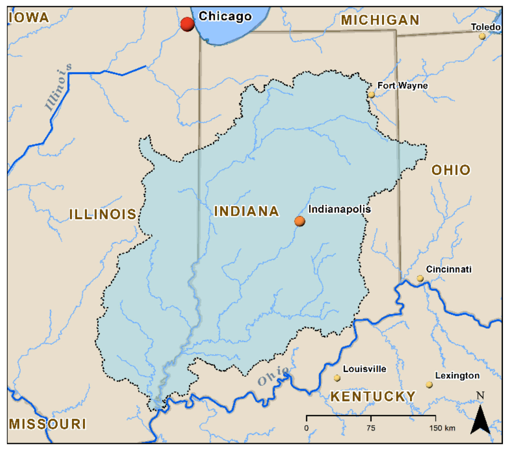
The domain for this study is the Wabash River Basin located in Midwest USA, which is the largest northern tributary of the Ohio River. The Wabash Basin drains over 90,000 km2, including most of the state of Indiana, part of eastern Illinois, and a small section of western Ohio (Figure 1). The watershed has a humid continental climate, with a mean annual temperature of 11.3 °C and mean annual precipitation of 122.7 cm over the 1971–2000 period.
2.2. Hydrologic Model
The Soil and Water Assessment Tool (SWAT) hydrological model (version 2012) was used to model the hydrologic cycle of the Wabash River Basin. SWAT is a semi-distributed watershed modeling program developed by the Agricultural Research Service (ARS) of the U.S. Department of Agriculture [20,21]. SWAT model construction requires inputs of hydrography, topography, soils, and land cover. For this study, model construction was facilitated by the program ArcSWAT [22], a SWAT interface for the geographic information systems (GIS) software ArcGIS. Further model setup included the choice of the curve number method [23] for estimating surface runoff and the Penman-Monteith method [24,25] for estimating potential evapotranspiration (PET) and actual evapotranspiration (AET).
The following sections outline the main steps in setting up the Wabash Basin SWAT model, including the gathering and pre-processing the required model inputs (Section 2.2.1) and the definition of hydrological response units (Section 2.2.2). Additional details on model setup, including the incorporation of tile drains [26,27,28,29,30,31], the aggregation of pond and lake area by subbasin, and the parameterization of reservoirs, are included in supplemental Text S1, Figures S1 and S2, and Tables S1 and S2.
2.2.1. Model Inputs
SWAT input datasets, including topography, delineated subbasins, soil properties, and land use/landcover (LULC) were compiled from multiple governmental agencies. Basin topography, in the form of a 10 m (1/3 arc-second) digital elevation model (DEM), was obtained from the National Elevation Dataset (NED) via the National Map Seamless Server (https://viewer.nationalmap.gov/basic/). Delineated subbasin polygons were obtained from the United States Geological Survey’s National Hydrography Dataset (NHD), with pre-defined streams and subbasins in the SWAT model corresponding to NHD 12-digit Hydrologic Unit Code (HUC) basins (Figure S1). Soil properties were obtained from the State Soil Geographic Database (STATSGO), which lumps soils into four hydrologic groups. Soils within the Wabash Basin are dominated by hydrologic groups B and C (Table S5).
Two land use/landcover (LULC) datasets were used to parameterize SWAT: (1) the 2001 National Land Cover Data (NLCD) [32] and (2) the National Agricultural Statistics Service (NASS) cropland data layers [33]. The NASS dataset contains detailed spatial data on agricultural crop types—information that is not available in the NLCD dataset. NASS, however, has missing data due to cloud cover and has less detailed classification for non-agricultural lands. The distribution of different crop types is potentially important for future SWAT model applications. For example, corn and soybeans have different optimal growth temperatures and will, therefore, respond differently to continued climate warming. Therefore, a combined NLCD and NASS LULC dataset was created for the Wabash Basin (Table S4; Figure S3). The primary LULC classes are soybean and corn, encompassing 26.1% and 25.3% of the area within the Wabash Basin. Details on the pre-processing steps for the LULC inputs can be found in supplemental Text S1.
Historical meteorological data and climate projections were obtained from the University of Notre Dame [34,35]. These gridded time series have a daily time step and include maximum temperature, minimum temperature, precipitation, and wind speed. The climate change projections have been statistically downscaled using the hybrid delta method (HD) for a subset of ten different global climate models (GCMs) from Phase 5 of the Coupled Model Intercomparison Project (CMIP5) under representative concentration pathways (RCPs) 4.5 and 8.5 (Table 1). RCP 4.5 represents a medium stabilization scenario; and RCP 8.5 represents a very high baseline emissions scenario [36]. The gridded time series have a 1/16° spatial resolution and were aggregated at the subbasin level for use in the SWAT model.
For the historical baseline, a single model simulation was completed using the gridded observation-based meteorological dataset (1915–2013). Three future periods, representing 30-year windows centered on the 2020s (2011–2040), 2050s (2041–2070), and 2080s (2071–2100), were used for the climate change scenario modeling. The 10-member GCM ensemble combined with the two emissions scenarios (RCPs 4.5 and 8.5) lead to a suite of 60 SWAT model runs for the climate change analysis (10 GCMs × 2 RCPs × three future periods), plus one SWAT model run for the historical baseline. Model runs were completed using Indiana University’s high-performance computing resources, with post-processing and model result visualization and analysis supported by Extreme Science and Engineering Discovery Environment (XSEDE) [37]. While the climate change projections are keyed to 30-year time periods, they have the same time series length as the baseline historical dataset due to the HD downscaling method, as described in [34,38]. For all model runs, the first 14 calendar years were used as the model spin-up period, resulting in 85 years (1929–2013) of daily model output. These relatively long time series have key advantages for estimating changes in extremes [38]; therefore, this dataset is well-suited for investigating changes in drought frequency and severity.
The 10-member GCM ensemble projects increases in temperature across all seasons, reaching a 5 °C increase in the mean annual temperature by the 2080s relative to the 1980s baseline under RCP 8.5. A comparison of annual and seasonal precipitation between the historical baseline and the three future periods, 2020s, 2050s, and 2080s, is presented in the results section, alongside the SWAT model water balance outputs. Further details on the projected changes in climate, the HD downscaling method, and the rationale for the selection of the 10-member GCM subset can be found in [34].
2.2.2. Hydrological Response Unit (HRU) Definition
In SWAT, hydrological response units (HRUs) are defined as unique combinations of land cover, soil, and/or slope classes within a subbasin. The HRU method is an effective way to simplify representation and simulation of watershed processes [39]. ArcSWAT allows users to specify two types of thresholds to define HRUs: percent-based and area-based. Higher thresholds result in fewer HRUs and thus shorter model run times. However, higher thresholds also result in greater generalization and thus a greater loss of information. Slope within the Wabash Basin is strongly correlated with landuse/landcover and soils; therefore, only one slope class was used, with slope set to the subbasin average. Based on an analysis of the trade-off between model simplicity versus information loss (see supplemental Text S1, Figure S4), area-based thresholds values were set as follows: land cover = 250 ha and soils = 650 ha, leading to a total of 6852 HRUs.
2.3. Model Calibration and Validation
After the initial data assimilation and model construction, the Wabash Basin SWAT model was calibrated and validated. Model calibration was completed in two stages. Stage 1 consisted of automated parameter regionalization, where a cascading methodology like the method outlined in [40] was used to set the calibration parameter values to an initial “best guess”. Parameter regionalization was completed in nine subbasin sets, where upstream reaches were parameterized with the “best guess” parameter sets before moving to the next downstream gauges (Figure S5, Table S6). The goal of this regionalization was to account for regional variations in the performance of initial parameter values, especially with regard to the most sensitive parameters. For each round in this cascading scheme, 500 model runs were completed. Stage 2 of the model calibration consisted of a multi-site, multi-criteria sequential uncertainty fitting (SUFI) procedure, similar to the method outlined by [41]. For Stage 2, two rounds were completed with 850 model iterations each. This two-stage calibration routine was completed using the R statistical programming software [42].
Both stages of the calibration routine use the same observed stream flow data and the same multi-criteria objection function, which are described in the following Section 2.3.1 and Section 2.3.2. Additional details on the calibration methodology, including (1) parameter constraints for deep aquifer recharge [43] and ground water recession constants [44,45], (2) initial parameter ranges, (3) parameter modification with Latin hypercube sampling [46], and (4) baseflow separation [47,48] and the detailed use of the multi-criteria objective function, are included in Text S2, Figures S4–S6, and Tables S7 and S8.
2.3.1. Stream Flow Calibration Sites
Observed stream flow records for all gauging stations within the Wabash River Basin were downloaded from the United States Geological Survey (USGS) using the R package waterData [49]. A time series plot of total annual stream flow at the downstream main-stem gauge (ID 03377500) was used to select the calibration and validation periods for the model, with the goal of including high flow and low flow years in both periods and maximizing the number of active gauging stations. The 8-year period from 1993–2000 was chosen as the calibration period, with 2001–2012 serving as the validation period, and 1981–1992 serving as the warm-up period (Figure S6).
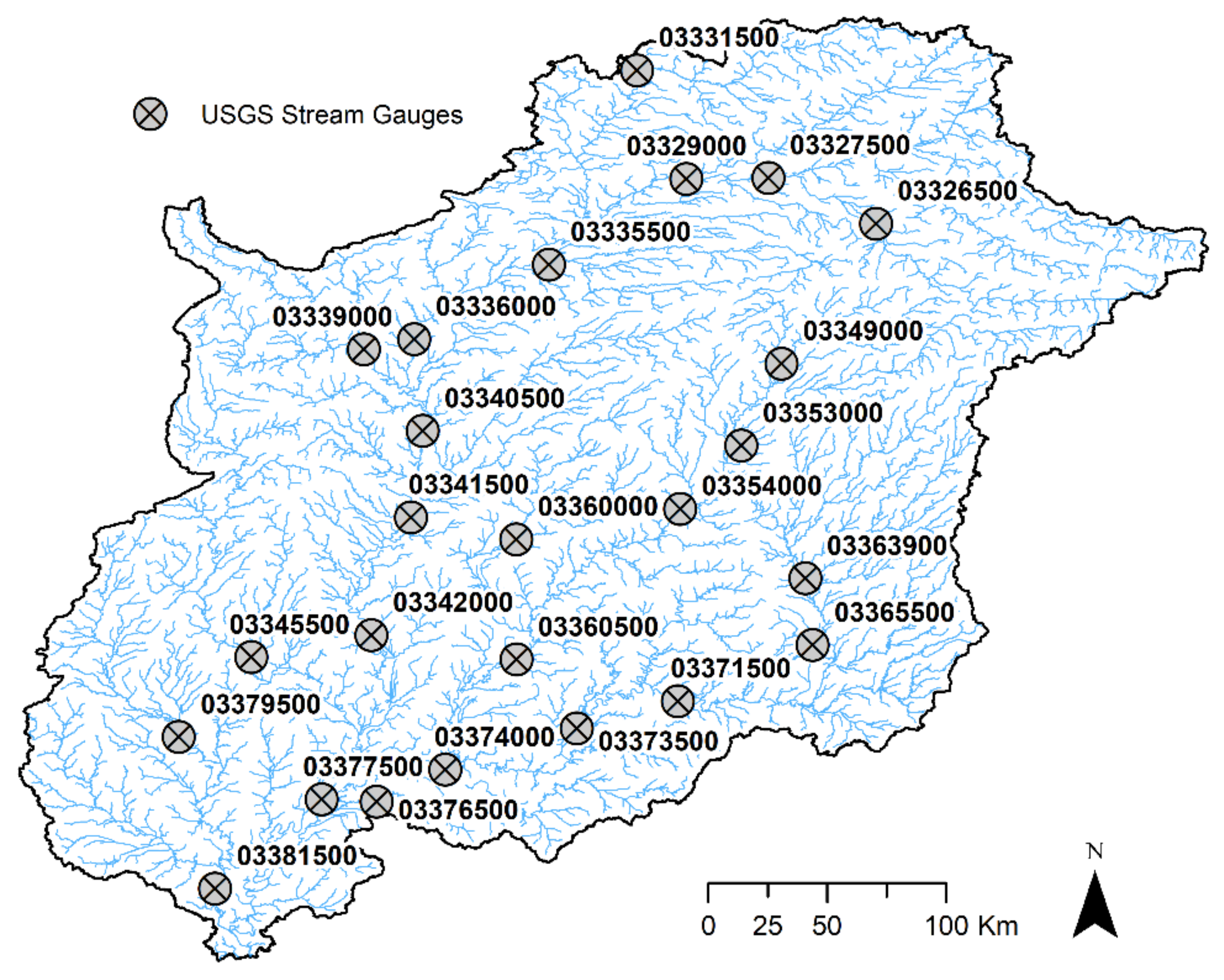
As part of the initial data screening, a subset of gauging stations within the Wabash Basin was chosen based on: (1) record completeness—no missing data 1993–2012, (2) spatial distribution—avoid clusters of gauging stations, and (3) proximity to lakes reservoirs—gauging stations with reservoir and lake effects were removed. The final selection included 25 gauging stations located throughout the Wabash River Basin, with drainage areas ranging from 1383 km2 to 74,164 km2 (Figure 2, Table 2).
2.3.2. Multi-Criteria Objective Function
The Nash–Sutcliffe efficiency criterion (NSE) [50] is often used to evaluate the performance of hydrological models. However, several shortcomings in the use of NSE as a single objective function have been pointed out [51] with one of the main problems being a greater emphasis on high flows. Therefore, other error metrics, including percent bias (PBIAS), root mean square error standard deviation ratio (RSR), and the volumetric efficiency criterion (VE) proposed by [51] were incorporated into a multi-criteria objective function (Table 3). VE was included because it represents the fraction of water delivered at the proper time. VE values range from 0 to 1, where 1 represents a perfect match. RSR and NSE are based on the minimization of the square of the residuals, while PBIAS and VE are based on the minimization of the absolute (VE) and relative (PBIAS) differences. These two error function types are complementary [52], and, thus, used together, help constrain parameter ranges, reduce model uncertainty, and increase model skill.
The “best” parameter set was chosen based on the minimization of a multi-criteria objective function, which incorporates the four different error metrics in Table 3. See Text S2 for additional details. For Stage 1 of model calibration, the objective function was calculated independently for each gauging station. For Stage 2, the objective function was calculated jointly for all 25 gauging stations by calculating a weighted mean for each error statistic, where the weights for each gauging station were equal to the ratio of the gauging station drainage (1383 km2 to 74,164 km2) area to the total drainage area upstream of all gauging stations (89,198 km2).
2.4. Quantification of Drought
To understand how climate change will impact drought, drought must first be quantified. A group of related drought indices—the standardized precipitation index (SPI) [54], the standardized soil moisture index (SSI) [55], and the standardized runoff index (SRI) [56]—are flexible, multi-scale indices that can be calculated over a range of timescales, typically 1 to 48 months. The multi-scale nature of these indices enables the quantification of both short-term and long-term drought characteristics. SPI, SSI, and SRI provide an assessment of meteorological, soil moisture, and hydrological drought, respectively. Hydrological drought is associated with deficiencies in the both surface water and groundwater; it is often diagnosed by streamflow drought. For this study, the quantification of hydrological drought focuses only on streamflow and does not consider groundwater storage.
The majority (66%) of the Wabash River Basin is cultivated agricultural land, and, in general, agricultural regions are the most sensitive to short-term droughts that coincide with critical crop development periods in July to August [19]. Therefore, SPI was calculated at 1- to 6-month timescales, and SSI and SRI were calculated at the 1-month timescale. The three drought indices—SPI, SSI, and SRI—were calculated using the same basic methodology:
- The time series of watershed-averaged precipitation, soil water content, and runoff were obtained from the SWAT model output for the historical baseline model simulation.
- The probability distributions of monthly precipitation, soil water content, and runoff were calculated separately for each month. Distribution fits were tested with the Shapiro–Wilk test. The gamma distribution produced a satisfactory fit for precipitation. No satisfactory distribution was found for soil moisture or runoff. Therefore, percentiles for soil moisture and runoff were estimated empirically, following recommendations in [56].
- Monthly time series of cumulative probabilities were calculated using the fitted distributions (for baseline and climate change scenarios) and then converted to z-values, representing the number of standard deviations below or above the mean of a normal distribution with a mean of 0 and a variance of 1.
The standardized index values provide a measure of drought severity, with more negative values indicating more severe drought conditions. Drought frequency was calculated as the fraction of years with moderately dry (moderate drought) to extremely dry (extreme drought) conditions, i.e., standardized index value of less than −1 (Table 4). The significance of changes in the frequency and severity of drought was then tested using the chi-square, Wilcoxon signed-rank, and Mann–Whitney U tests. The chi-square test was used to test for significant changes in drought frequency. The Wilcoxon signed-rank test [57] was used to test for significant shifts in the drought indices toward higher (wetter conditions) or lower (drier conditions) values. The Mann–Whitney U test [58] was used to test for significant changes in median drought severity.
The Wilcoxon signed-rank test is a nonparametric statistical hypothesis test to determine if there is a significant difference between two matched samples, where the matched samples correspond to the drought indices calculated from (1) the historical baseline and (2) the climate change scenarios. The Mann–Whitney U test is an alternate version of the Wilcoxon signed-rank test and is used to determine if there is a significant difference between to independent (i.e., unmatched) samples. For this study, the independent samples corresponded to the subset of drought index values (i.e., SPI, SSI, SRI values less than −1) for (1) drought events in the historical baseline and (2) drought events in the climate change scenarios.
To further investigate climate change impacts on the drought regime, the relationships between the different drought types were analyzed with bivariate correlation analysis and multiple linear regression. Identifying relationships between different drought types provides a basis for understanding how drought propagates through the hydrologic system, specifically the propagation of meteorological drought into soil moisture or hydrological drought. Therefore, SSI and SRI at the 1-month timescale were used as the dependent variables (predictands) with SPI at 1- to 6-month timescales used as the independent variables (predictors). Combinations of predictor variables were tested using automatic stepwise (combined forward and backward) regression analysis, with final model selection based on the Akaike Information Criterion (AIC) [59].
3. Results
The following sections present the model calibration and validation (Section 3.1) and the results of the climate change scenario modeling, including climate change impacts on the annual and intra-annual water balance (Section 3.2) and the frequency and severity of drought (Section 3.3). Further analysis using multiple linear regression models to investigate how climate warming impacts the relationship between meteorological and soil moisture and hydrological drought is included in Section 3.4.
3.1. Model Calibration and Validation
The SWAT model was calibrated with the 1993–2000 period and validated with the 2001–2012 period. The error statistics for the calibration and validation periods for the “best” model simulation are included in Tables S9 and S10. For the calibration period, PBIAS was below the calibration target of ±25% for all 25 gauging stations, and the majority (23/25) of stations met the calibration goal for NSE and RSR. All calibration targets were met at the downstream main-stem gauging station (Wabash River at Mt Carmel—USGS gauge 03377500) in both the calibration and validation periods (Tables S9 and S10; Figures S8 and S9).
Overall, model performance in the validation period is similar to the calibration period. The main-stem gauging station (03377500) had a higher PBIAS value compared to the calibration period (−3.3% calibration, +7.0% validation). This pattern is similar for the other stream flow gauges; however, only three out of the 25 gauging stations have PBIAS values higher than the calibration target of ±25%. This tendency toward higher PBIAS values indicates an over-prediction of stream flow in the validation period compared to the calibration period. While the cause of the over-prediction in the validation period is unclear, it may be due to changing land and water use patterns, which were not incorporated into the model. For this study, the model outputs for the full 61-member model ensemble are analyzed in terms of the sensitivity to climate change, focusing on the relative change rather than on absolute change. With this focus, the implications of the higher PBIAS values are minimal.
3.2. Climate Change Impacts on Annual and Intra-Annual Water Balance
A water balance analysis was completed for each of the 61 scenarios (one historical baseline; 60 climate change). The water balance components of interest for this study include the input precipitation and the model outputs of the amount of precipitation falling as snow, AET, soil moisture, ground water recharge, and stream flow. Water balance results for individual GCMs are not shown, but rather lumped by RCP (4.5, and 8.5) and period (2020s, 2050s, and 2080s) and reported by the inter-model spread and the ensemble mean for simplicity. Results are presented as the percent change from the historical baseline (((future - baseline)/baseline) × 100) at both the annual (Figure 3) and monthly (Figure 4) time scale.
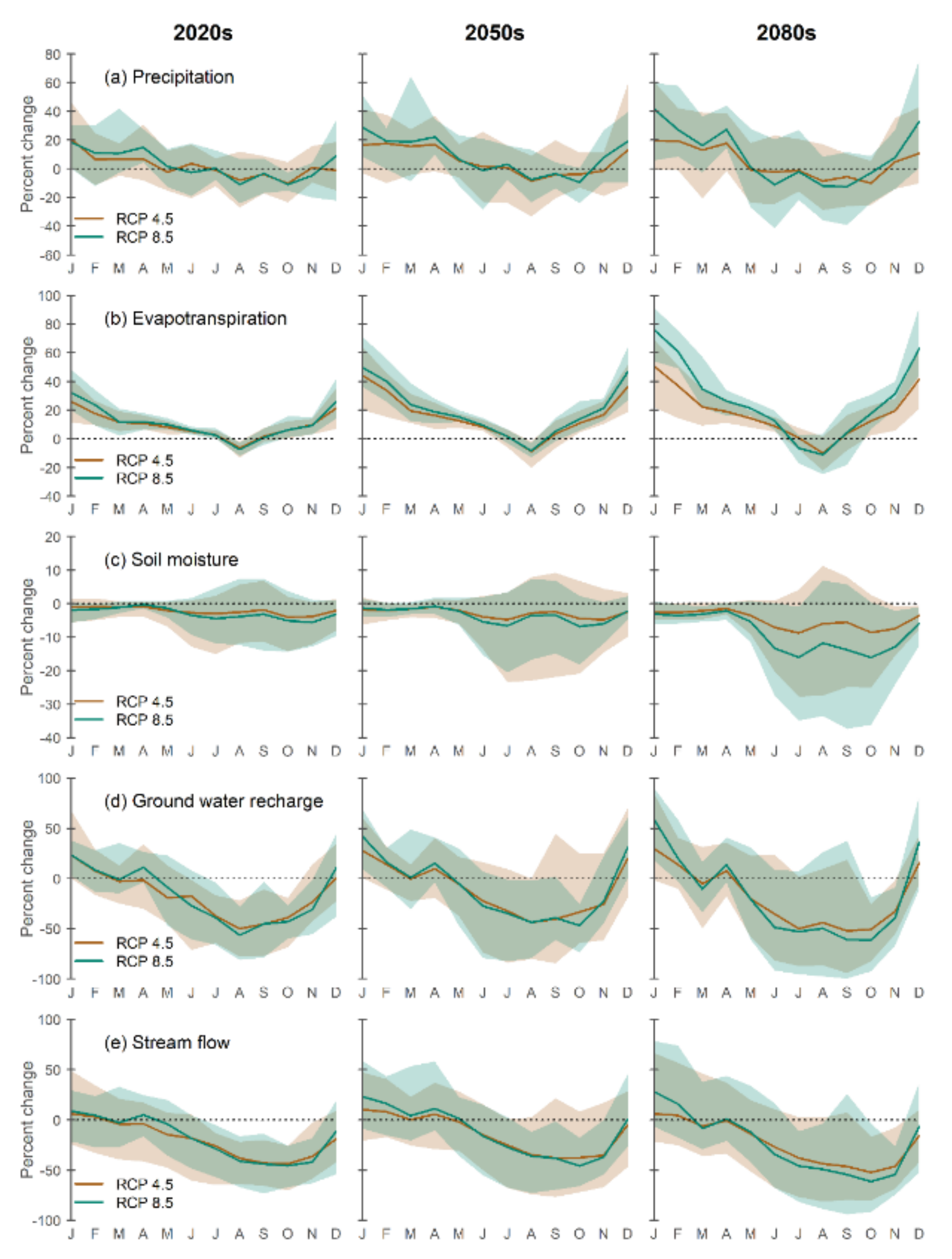
Based on statistically downscaled climate projections, there is high certainty that regional temperatures will increase in the future [34]; however, the direction and magnitude of precipitation change is less certain. The inter-model variability of projected precipitation is high and increases from near future (2020s) to far future (2080s) (Figure 3a). In general, precipitation in winter (December, January, and February) is projected to increase while precipitation in late summer and fall (August, September, and October) is likely to exhibit no change or decrease slightly (Figure 4a).
Water balance variables that are closely linked to temperature, i.e., snow and AET, exhibit consistent changes and a low amount of inter-model variability (Figure 3 and Figure 4). The amount of precipitation falling as snow decreases (Figure 3b) while AET increases (Figure 3c). As expected, the largest increases in AET occur in the far future (2080s) under the high emissions scenario (RCP 8.5). Seasonally, AET increases the most in winter (December to February) and decreases slightly or exhibits no substantial change during late summer and early fall (July to August; Figure 4b). The seasonal pattern in the AET change is related to seasonal water availability. Increasing temperatures cause PET to increase in all months (results not shown). AET, however, is dependent on both the PET and water availability. If little or no water is available, AET will be small or zero even when PET is high.
Soil moisture, ground water recharge, and stream flow are more closely linked to precipitation than to temperature. The mean annual values of soil moisture, ground water recharge, and stream flow exhibit both increases and decreases relative to the historical baseline, due to the high inter-model variability in precipitation (Figure 3d–f). Seasonally, ground water recharge, stream flow, and soil moisture exhibit a pattern of decreased water availability in summer (June, July, August) and fall (September, October, November; Figure 4c–e).
3.3. Projected Changes in Meteorological, Soil Moisture, and Hydrological Drought
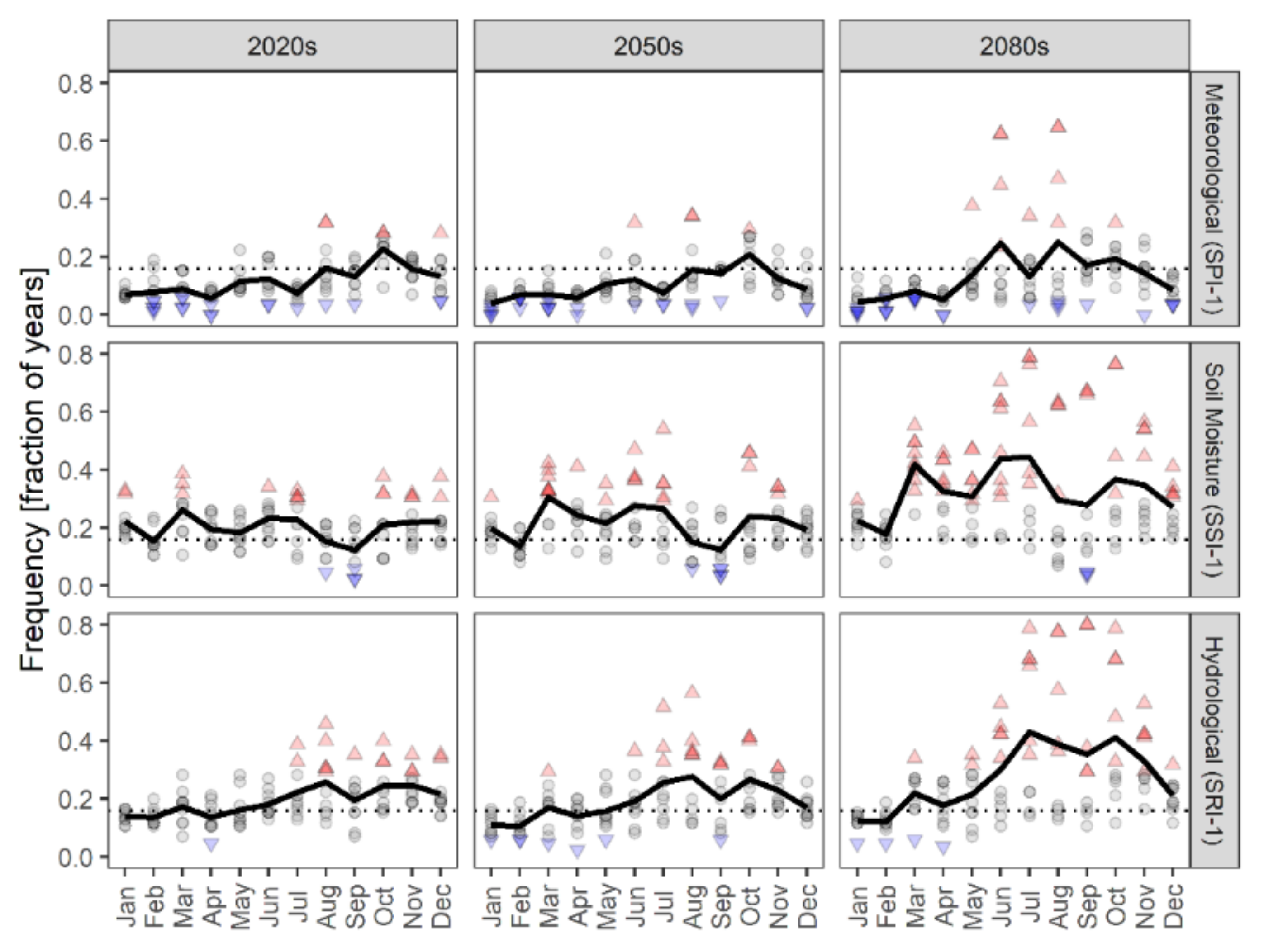
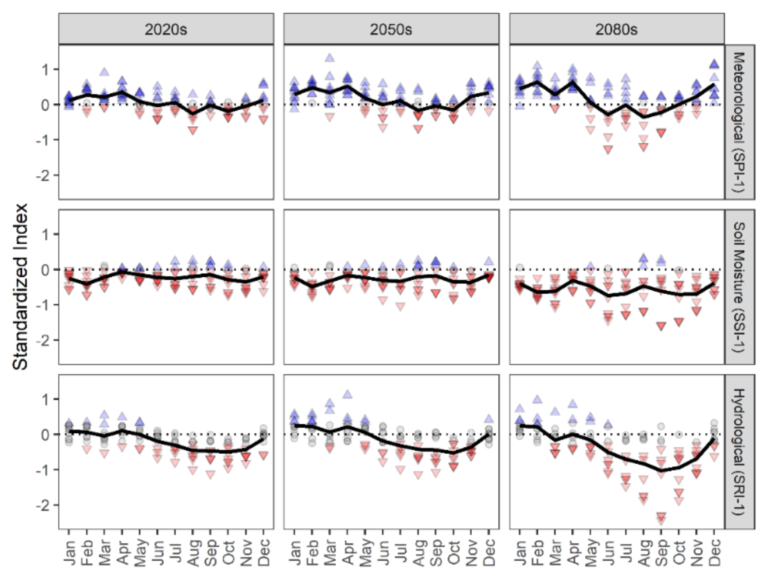
Soil moisture and hydrological droughts become significantly more frequent in the far future under both emissions scenarios, particularly during the summer months (Figure 5 and Figure S10). Meteorological droughts, however, exhibit either decreasing frequency or no significant change, with relatively few GCMs showing a significant increase in meteorological drought frequency. Changes in monthly drought indexes, SPI, SSI, and SRI, mirror the patterns shown in the results for the monthly water balance presented in Section 3.2, with a shift toward drier conditions (lower SSI and SRI values) in summer and fall (Figure 6 and Figure S11) and higher precipitation (higher SPI values) in winter.
Despite the increased frequency of soil moisture and hydrological drought (Figure 5) and the general shift toward lower SSI and SRI values (Figure 6) there is, in general, no significant change in the mean severity of moderate to severe drought events (Figures S12 and S13). Therefore, while soil moisture and hydrological droughts will likely be more frequent in the future, the average drought severity will not be significantly different from the historical baseline.
3.4. Climate Warming Impacts on Relationship between Drought Types
Soil moisture and runoff over 1-month timescales, represented by SSI-1 and SRI-1, exhibit the strongest correlations with precipitation over 3- to 4-month timescales (SPI-3, SPI-4; Table 5). In the historical baseline period, the magnitude of SPI, SSI and SRI are also closely linked, and near-normal precipitation results in near-normal soil moisture and runoff. However, as the climate warms, this relationship changes, and there is a shift toward lower soil moisture and lower runoff for the same near-normal amount of precipitation (Figures S14 and S15).
This shift toward lower runoff and lower soil moisture indicates an amplification of soil moisture and hydrological drought due to climate warming. To quantify the degree of drought amplification, multiple linear regression (MLR) models were used. Since the relationships between SPI and SSI/SRI vary seasonally (Figures S14 and S15), separate MLR models were created for each month, for a total of 732 MLR models each for SSI and SRI (61 SWAT simulations × 12 months). The final MLR models account for an average of 71% and 78% of the variability in SSI and SRI, respectively (Figure S16).
From these MLR models, the y-intercept represents the predicted SSI or SRI from an SPI of 0 and thus provides a simple estimate of the degree of drought amplification for each of the climate change scenarios. As expected, the y-intercept is non-significant and near zero for the baseline historical 1980s, when near-normal precipitation (SPI of 0) corresponds to near-normal soil moisture and runoff (SSI and SRI of 0). For the three future periods (2020s, 2050s, and 2080s), however, the y-intercept has a negative value and is significant at the 5% level in most months (Figure S17), indicating that the shift toward lower soil moisture and lower runoff for the same near-normal amount of precipitation is statistically significant.
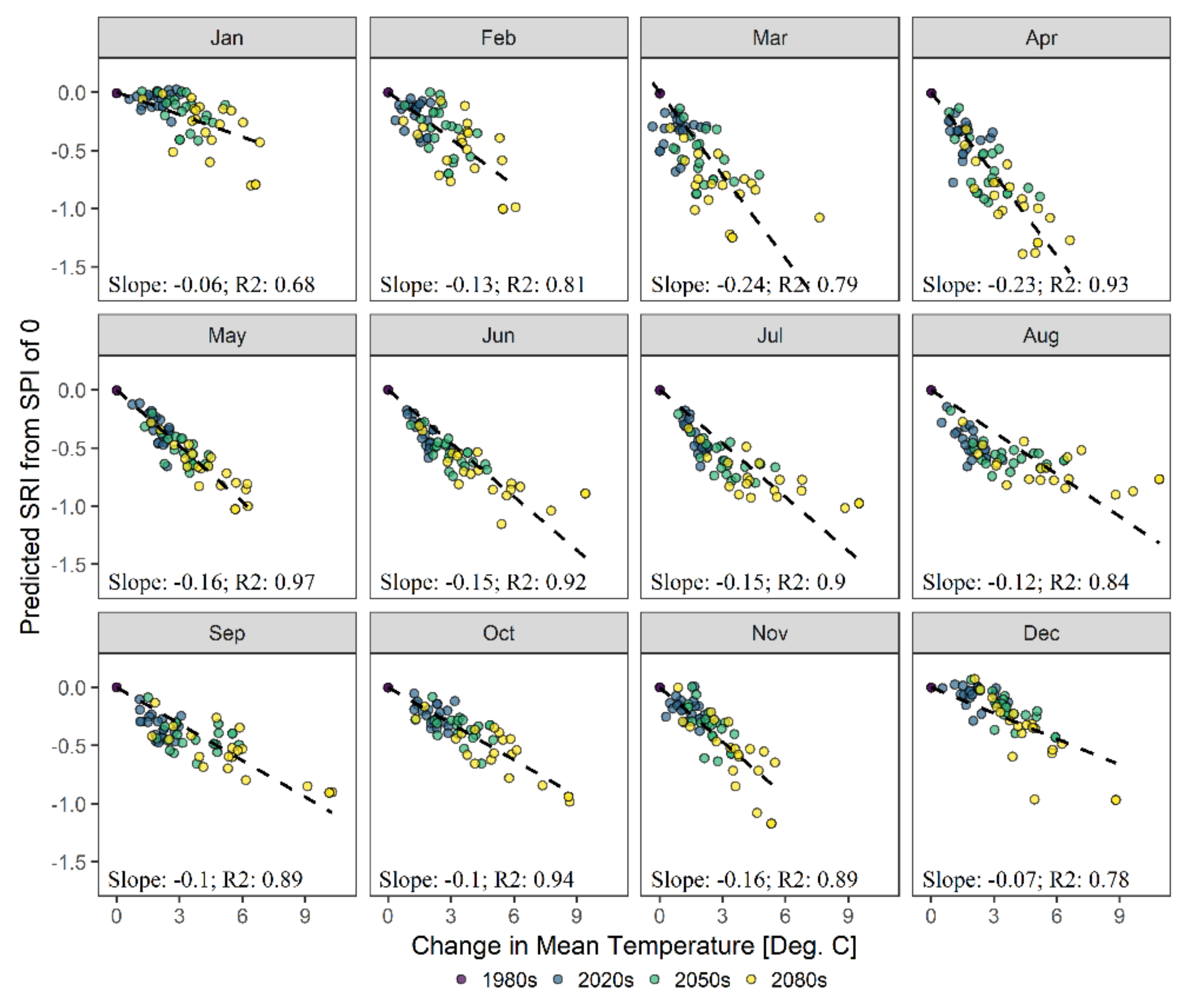
Plotting the y-intercepts from the MLR models versus change in monthly mean temperature shows that, in these model simulations, climate warming is driving the amplification of soil moisture and hydrological drought. Further, the rate of this amplification, in terms of the change in standardized drought index per °C (SI °C−1), can be quantified using the simple linear model fits shown on Figure 7 and Figure 8. For soil moisture, drought amplification from climate warming is greatest in the months of February, March, and April. For runoff, it is greatest in the months of March and April. The implications of this are clarified by framing the amplification in terms of drought severity. In the historical baseline period, moderate meteorological droughts propagate into moderate soil moisture and hydrological droughts. A slope of −0.1 SI °C−1 indicates that, with 5 °C of warming, moderate meteorological droughts will be amplified into severe soil moisture and hydrological droughts. Further, under 5 °C of warming and a slope of −0.2 SI °C−1, moderate soil moisture and hydrological droughts are likely to occur even with near-normal precipitation.
4. Discussion
While several recent studies have used hydrological models to investigate climate change impacts on meteorological, soil moisture, and hydrological drought [13,14,61], no previous studies have specifically focused on short-term drought events and identified intra-annual patterns in the drought response to climate change. In this study, a large ensemble of 61 hydrological models was combined with an analysis of monthly drought indices and MLR models. Climate change projections show increases in temperature and in the seasonality of precipitation, leading to increased frequency of soil moisture drought and hydrological drought. Hydrological modeling results show that climate warming amplifies soil moisture and hydrological drought, with the same amount of precipitation yielding significantly lower soil moisture and significantly lower runoff in the future than in the past.
The role of above-average temperatures in the amplification of soil moisture and hydrological drought has been documented by previous studies in California [16], central and western Europe [15], and the Iberian Peninsula [62]. In this study, we focus on a historically water-rich agricultural region within the US Midwest and quantify drought amplification in terms of the increase in drought severity per degree increase in monthly mean temperature. Results show that the degree of drought amplification varies seasonally. For soil moisture, the seasonal variation is related to the local hydroclimatology. With the same near-normal precipitation, climate warming amplifies soil moisture drought more in energy-limited months (e.g., March–April, Figure 7) when the PET and AET are near equal than in moisture-limited months (e.g., August–October; Figure 7) when the PET is substantially higher than the AET.
Climate warming also amplifies hydrological droughts most in spring (March–April, Figure 8). However, the impact of climate warming on hydrological drought is lowest in winter (December–January, Figure 8), likely due to the added complexity of snow accumulation and melt. Even with the seasonal variations, results clearly show that temperature plays a significant role in the amplification of soil moisture and hydrological droughts. Under 5 °C of warming, moderate meteorological droughts will be amplified into severe soil moisture and streamflow droughts for most months of the year. While the results presented here are region-specific and dependent on the local hydroclimatology, the methodology could be transferred to other regions and used to understand how the relationship between meteorological drought and soil moisture/hydrological drought will change under continued climate warming.
Like all hydrological models, the calibrated SWAT model used in this study is a simplified numerical representation of the natural flow system, and it cannot duplicate the natural flow system exactly. Uncertainties are inherent in model structure, input data, parameterization, and GCM selection. However, the model is physics-based and assessment with multiple error statistics indicates good performance (Tables S9 and S10). Attributing model uncertainty among the different sources is difficult and beyond the scope of this paper. Additionally, land use change and climate change mitigation were assumed to be constant in both the baseline and future climate change scenarios. Incorporation of land use change and climate change mitigation is beyond the scope of this paper but is a promising direction for future research.
Additional limitations of this study stem from aggregation of the water balance and drought indices to the watershed scale. The response of soil moisture drought and hydrological drought to climate change may vary spatially due to heterogeneity of the catchment’s physical properties, e.g., land use, soil type, and geology. Additionally, this study only analyzed total soil moisture. Shallow soil moisture and deep soil moisture may exhibit different responses to climate change [63,64]. A useful extension of this work would be to (1) investigate if the physical properties of the catchment control the degree of soil moisture and hydrological drought amplification under climate warming and (2) determine if shallow and deep soil moisture exhibit different responses to climate warming.
5. Conclusions
In climate change projections, the uncertainty in precipitation is inherently higher than the uncertainty in temperature. Since precipitation dominates the hydrologic regime in water-rich regions, the uncertainty in projected precipitation carries through to uncertainty in the direction and magnitude of future change in the hydrological regime. The analysis presented here, however, separates out the role of temperature and shows that increased temperatures cause an amplification of soil moisture and hydrological drought. In general, for this study region, the frequency and severity of meteorological drought does not change significantly from the frequency and severity of meteorological droughts in the historical period. However, our analysis shows that while moderate meteorological droughts propagate into moderate soil moisture and hydrological droughts in the baseline period, this relationship changes in the future periods, and moderate meteorological droughts will propagate into severe soil moisture and hydrological droughts under 5 °C of warming.
Supplementary Materials
The following are available online at https://www.mdpi.com/2073-4441/12/1/181/s1, Text S1: Model Construction, Text S2: Model Calibration, Figure S1: Tile drained agricultural land, Figure S2: Subbasin area draining to lakes, ponds, or wetlands, Figure S3: Reclassified land use/land cover, Figure S4: Average relative error of aggregation (aREA), Figure S5: Parameter regionalization zones, Figure S6: Warm up, calibration, and validation periods, Figure S7: Initial values for the proportion of recharge to the deep aquifer, Figure S8: Observed versus simulated stream flow–calibration period, Figure S9: Observed versus simulated stream flow–validation period, Figure S10: Projected change in the frequency of moderate to extreme meteorological, soil moisture, and hydrological droughts under representative concentration pathway (RCP) 4.5, Figure S11: Monthly means of the standardized indices (SPI-1, SSI-1, SRI-1) under RCP 4.5, Figure S12: Mean drought severity under RCP 4.5, Figure S13: Mean drought severity under RCP 8.5, Figure S14: Point density plots of SPI-3 versus SSI-1, Figure S15: Point density plots of SPI-3 versus SRI-1, Figure S16: Multiple linear regression (MLR) model performance for (a) SSI and (b) SRI, Figure S17: Count of MLR models with significant y-interceptstitle, Table S1: Tile drainage parameters, Table S2: Lakes and reservoirs in SWAT model, Table S3: Land cover/land use reclassification, Table S4: Reclassified land use, Table S5: Percent area of soil hydrologic groups, Table S6: Cascading calibration scheme, Table S7: Parameter modification method and initial ranges—Stage 1, Table S8: Parameter modification method and initial ranges—Stage 2, Table S9: Calibration period error statistics, Table S10: Validation period error statistics, Table S11: Tabular version of Figure 3.
Author Contributions
Conceptualization, J.R.D. and C.Z.; Methodology, J.R.D. and C.Z.; Software, J.R.D.; Validation, J.R.D.; Formal analysis, J.R.D.; Investigation, J.R.D.; Resources, C.Z.; Data curation, J.R.D.; Writing—Original draft preparation, J.R.D.; Writing—Review and editing, J.R.D. and C.Z.; Visualization, J.R.D.; Supervision, C.Z.; Project administration, C.Z.; Funding acquisition, C.Z. All authors have read and agreed to the published version of the manuscript.
Funding
This research was funded by Indiana University through the Grand Challenges Prepared for Environmental Change project, grant number 23-272-65 and through an Extreme Science and Engineering Discovery Environment (XSEDE) Startup Allocation and Extended Collaboration Support, grant number EAR190021.
Acknowledgments
This project was partly supported by the Environmental Resilience Institute, funded by Indiana University’s Prepared for Environmental Change Grand Challenge initiative. This work used XSEDE resources, including Jetstream at Indiana University’s Pervasive Technology Institute and Stampede2 at the Texas Advanced Computing Center, which are supported by National Science Foundation grant number ACI-1548652. We thank Sudhakar Pamidighantam, Eroma Abeysinghe, Jun Wang, Marcus Christie, Suresh Marru, Marlon Pierce, Alan Walsh, and Kent Milfeld for their assistance in using Indiana University’s High Performance Computing systems and XSEDE resources and in developing a science gateway, which was made possible through the XSEDE Extended Collaborative Support Service (ECSS) program.
Conflicts of Interest
The authors declare no conflict of interest.
References
- Palmer, W.C. Meteorological Drought; United States Department of Commerce: Washington, DC, USA, 1965.
- Dracup, J.A.; Lee, K.S.; Paulson, E.G. On the definition of droughts. Water Resour. Res. 1980, 16, 297–302. [Google Scholar] [CrossRef]
- Van Loon, A.F. Hydrological drought explained. Wiley Interdiscip. Rev. Water 2015, 2, 359–392. [Google Scholar] [CrossRef]
- Rippey, B.R. The U.S. drought of 2012. Weather Clim. Extrem. 2015, 10, 57–64. [Google Scholar] [CrossRef] [Green Version]
- Sheffield, J.; Wood, E.F. Drought: Past Problems and Future Scenarios; Earthscan: London, UK, 2011. [Google Scholar]
- Feyen, L.; Dankers, R. Impact of global warming on streamflow drought in Europe. J. Geophys. Res. Atmos. 2009, 114, 1–17. [Google Scholar] [CrossRef]
- Dai, A. Drought under global warming in observations and models. Nat. Clim. Chang. 2013, 3, 52–58. [Google Scholar] [CrossRef]
- Intergovernmental Panel on Climate Change (IPCC). Climate Change 2013: The Physical Science Basis. Contribution of Working Group I to the Fifth Assessment Report of the Intergovernmental Panel on Climate Change; Stocker, T.F., Qin, G.-K., Plattner, M., Tignor, S.K., Allen, J., Boschung, A., Nauels, Y., Xia, V., Bex, D., Midgley, P.M., Eds.; Cambridge University Press: Cambridge, UK, 2013; p. 1535. [Google Scholar]
- Wehner, M. Projections of future drought in the continental United States and Mexico. J. Hydrometeorol. 2011, 12, 1359–1377. [Google Scholar] [CrossRef]
- Swain, S.; Hayhoe, K. CMIP5 projected changes in spring and summer drought and wet conditions over North America. Clim. Dyn. 2015, 44, 2737–2750. [Google Scholar] [CrossRef]
- Seager, R.; Ting, M.; Held, I.; Kushnir, Y.; Lu, J.; Vecchi, G.; Huang, H.; Harnik, N.; Leetmaa, A.; Lau, N.; et al. Model projections of an imminent transition to a more arid climate in southwestern North America. Science 2007, 316, 1181–1184. [Google Scholar] [CrossRef]
- Gutzler, D.S.; Robbins, T.O. Climate variability and projected change in the western United States: Regional downscaling and drought statistics. Clim. Dyn. 2011, 37, 835–849. [Google Scholar] [CrossRef]
- Wang, D.; Hejazi, M.; Cai, X.; Valocchi, A.J. Climate change impact on meteorological, agricultural, and hydrological drought in central Illinois. Water Resour. Res. 2011, 47, W09527. [Google Scholar] [CrossRef] [Green Version]
- Kang, H.; Sridhar, V. Combined statistical and spatially distributed hydrological model for evaluating future drought indices in Virginia. J. Hydrol. Reg. Stud. 2017, 12, 253–272. [Google Scholar] [CrossRef]
- Teuling, A.J.; Van Loon, A.F.; Seneviratne, S.I.; Lehner, I.; Aubinet, M.; Heinesch, B.; Bernhofer, C.; Grunwald, T.; Prasse, H.; Spank, U. Evapotranspiration amplifies European summer drought. Geophys. Res. Lett. 2013, 40, 2071–2075. [Google Scholar] [CrossRef]
- Diffenbaugh, N.S.; Swain, D.L.; Touma, D. Anthropogenic warming has increased drought risk in California. Proc. Natl. Acad. Sci. USA 2015, 112, 3931–3936. [Google Scholar] [CrossRef] [PubMed] [Green Version]
- Verdon-Kidd, D.C.; Kiem, A.S. Quantifying drought risk in a nonstationary climate. J. Hydrometeorol. 2010, 11, 1019–1031. [Google Scholar] [CrossRef]
- Smidt, S.J.; Kendall, A.D.; Hyndman, D.W. Increased dependence on irrigated crop production across the CONUS (1945–2015). Water 2019, 11, 1458. [Google Scholar] [CrossRef] [Green Version]
- Zipper, S.C.; Qiu, J.; Kucharik, C.J. Drought effects on US maize and soybean production: Spatiotemporal patterns and historical changes. Environ. Res. Lett. 2016, 11, 094021. [Google Scholar] [CrossRef]
- Arnold, J.G.; Williams, J.R.; Maidment, D.R. Continuous-time water and sediment-routing model for large basins. J. Hydraul. Eng. 1995, 121, 171–183. [Google Scholar] [CrossRef]
- Arnold, J.G.; Srinivasan, R.; Muttiah, R.S.; Williams, J.R. Large area hydrologic modeling and assessment part I: Model development. J. Am. Water Resour. Assoc. 1998, 34, 73–89. [Google Scholar] [CrossRef]
- Winchell, M.; Srinivasan, R.; Di Luzio, M.; Arnold, J. ArcSWAT Interface for SWAT 2005: User’s Guide; Blackland Research Center: Temple, TX, USA, 2008; pp. 1–453. [Google Scholar]
- United States Department of Agriculture (USDA). Urban Hydrology for Small Watersheds; Engineering Division, Soil Conservation Service, USDA: Washington, DC, USA, 1986.
- Monteith, J.L. Evaporation and environment. Symp. Soc. Exp. Biol. 1965, 19, 205–234. [Google Scholar]
- Ritchie, J.T. Model for predicting evaporation from a row crop with incomplete cover. Water Resour. Res. 1972, 8, 1204–1213. [Google Scholar] [CrossRef] [Green Version]
- Beik, S.E. Tile Drain Installation and Repair. In Indiana Drainage Handbook—October 1999 Update Package; Burke, C.B., Ed.; State of Indiana: Indianapolis, IN, USA, 1999; pp. 118–130. [Google Scholar]
- Kalita, P.; Algoazany, A.; Mitchell, J.; Cooke, R.; Hirschi, M. Subsurface water quality from a flat tile-drained watershed in Illinois, USA. Agric. Ecosyst. Environ. 2006, 115, 183–193. [Google Scholar] [CrossRef]
- Sugg, Z. Assessing U.S. Farm Drainage: Can GIS Lead to Better Estimates of Subsurface Drainage Extent? World Resources Institute. Available online: http://pdf.wri.org/assessing_farm_drainage.pdf (accessed on 29 October 2019).
- Srinivasan, R.; Zhang, X.; Arnold, J. SWAT ungauged: Hydrological budget and crop yield predictions in the Upper Mississippi River Basin. Trans. ASABE 2010, 53, 1533–1546. [Google Scholar] [CrossRef]
- Kalcic, M.M.; Frankenberger, J.; Chaubey, I. Spatial optimization of six conservation practices using SWAT in tile-drained agricultural watersheds. J. Am. Water Resour. Assoc. 2015, 51, 956–972. [Google Scholar] [CrossRef]
- Guo, T.; Gitau, M.; Merwade, V.; Arnold, J.; Srinivasan, R.; Hirschi, M.; Engel, B. Comparison of performance of tile drainage routines in SWAT 2009 and 2012 in an extensively tile-drained watershed in the Midwest. Hydrol. Earth Syst. Sci. 2018, 22, 89–110. [Google Scholar] [CrossRef] [Green Version]
- Homer, C.; Dewitz, J.; Fry, J.; Coan, M.; Hossain, N.; Larson, C.; Herold, N.; McKerrow, A.; VanDriel, J.N.; Wickham, J. Completion of the 2001 National Land Over Database for the conterminous United States. Photogramm. Eng. Remote Sens. 2007, 73, 337–341. [Google Scholar]
- Boryan, C.; Yang, Z.; Mueller, R.; Craig, M. Monitoring US Agriculture: The US Department of Agriculture, National Agricultural Statistics Service Cropland Data Layer Program. Geocarto Int. 2011, 26, 341–358. [Google Scholar] [CrossRef]
- Byun, K.; Hamlet, A.F. Projected changes in future climate over the Midwest and Great Lakes region using downscaled CMIP5 ensembles. Int. J. Climatol. 2018, 38, 531–553. [Google Scholar] [CrossRef]
- CMIP5 in CCIA. Available online: http://www.crc.nd.edu/~kbyun/CMIP5_IN_CCIA.html (accessed on 29 October 2019).
- Van Vuuren, D.P.; Edmonds, J.; Kainuma, M.; Riahi, K.; Thomson, A.; Hibbard, K.; Hurtt, G.C.; Kram, T.; Krey, V.; Lamarque, J.; et al. The representative concentration pathways: An overview. Clim. Chang. 2011, 109, 5–31. [Google Scholar] [CrossRef]
- Towns, J.; Cockerill, T.; Dahan, M.; Foster, I.; Gaither, K.; Grimshaw, A.; Hazlewood, V.; Lathrop, S.; Lifka, D.; Peterson, G.D.; et al. XSEDE: Accelerating scientific discovery. Comput. Sci. Eng. 2014, 16, 62–74. [Google Scholar] [CrossRef]
- Byun, K.; Chiu, C.-M.; Hamlet, A.F. Effects of 21st century climate change on seasonal flow regimes and hydrologic extremes over the Midwest and Great Lakes region of the US. Sci. Total Environ. 2019, 650, 1261–1277. [Google Scholar] [CrossRef]
- Gassman, P.W.; Reyes, M.R.; Green, C.H.; Arnold, J.G. The Soil and Water Assessment Tool: Historical development, applications, and future research directions. Trans. ASABE 2007, 50, 1211–1250. [Google Scholar] [CrossRef] [Green Version]
- Xue, X.; Zhang, K.; Hong, Y.; Gourley, J.J. New multisite cascading calibration approach for hydrological models: Case study in the Red River Basin using the VIC model. J. Hydrol. Eng. 2015, 21, 05015019. [Google Scholar] [CrossRef] [Green Version]
- Abbaspour, K.C.; Vejdani, M.; Haghighat, S. SWAT-CUP2: SWAT Calibration and Uncertainty Programs Manual Version 2. Department of Systems Analysis, Integrated Assessment and Modelling (SIAM); Eawag Swiss Federal Institute of Aquatic Science and Technology: Duebendorf, Switzerland, 2011; p. 106. [Google Scholar]
- R Development Core Team. R: A Language and Environment for Statistical Computing; R Foundation for Statistical Computing: Vienna, Austria, 2014. [Google Scholar]
- Wittman, J. Water and Economic Development in Indiana: Modernizing the State’s Approach to A Critical Resource. INTERA for the Indiana Chamber of Commerce. 2014. Available online: https://www.indianachamber.com/wp-content/uploads/2017/09/WaterStudyReport2014LoRes.pdf (accessed on 29 October 2019).
- Gustard, A.; Demuth, S. Manual on Low-Flow Estimation and Prediction; Operational Hydrology Report No. 50; World Meteorological Organisation: Geneva, Switzerland, 2008; p. 136. [Google Scholar]
- Koffler, D.; Gauster, T.; Laaha, G. Lfstat: Calculation of Low Flow Statistics for Daily Stream Flow Data. R Package Version 0.9.4. Available online: https://cran.r-project.org/web/packages/lfstat/index.html (accessed on 29 October 2019).
- Carnell, R. Lhs: Latin Hypercube Samples. R Package Version 1.0.1. Available online: https://cran.r-project.org/web/packages/lhs/index.html (accessed on 29 October 2019).
- Chapman, T.B.; Maxwell, A. Baseflow separation—Comparison of numerical methods with tracer experiments. In Hydrology and Water Resources Symposium 1996: Water and the Environment: Preprints of Papers; Institution of Engineers: ACT, Australia, 1996. [Google Scholar]
- Eckhardt, K. How to construct recursive digital filters for baseflow separation. Hydrol. Process. 2005, 19, 507–515. [Google Scholar] [CrossRef]
- Ryberg, K.R.; Vecchia, A.V. Waterdata: Retrieval, Analysis, and Anomaly Calculation of Daily Hydrologic Time Series Data. R Package Version 1.0.8. Available online: https://cran.r-project.org/web/packages/waterData/ (accessed on 29 October 2019).
- Nash, J.E.; Sutcliffe, J.V. River flow forecasting through conceptual models. Part I: A discussion of principles. J. Hydrol. 1970, 10, 282–290. [Google Scholar] [CrossRef]
- Criss, R.E.; Winston, W.E. Do Nash values have value? Discussion and alternate proposals. Hydrol. Process. 2008, 22, 2723–2725. [Google Scholar] [CrossRef]
- Muleta, M.K. Model performance sensitivity to objective function during automated calibrations. J. Hydrol. Eng. 2012, 17, 756–767. [Google Scholar] [CrossRef]
- Moriasi, D.N.; Arnold, J.G.; Van Liew, M.W.; Bingner, R.D.; Harmel, R.D.; Leith, T.L. Model evaluation guidelines for systematic quantification of accuracy in watershed simulations. Trans. ASABE 2007, 50, 885–900. [Google Scholar] [CrossRef]
- McKee, T.B.; Doesken, N.J.; Kleist, J. Drought Monitoring with Multiple Time Scales Proceeding of the Ninth Conference on Applied Climatology; American Meteorological Society: Boston, MA, USA, 1995. [Google Scholar]
- AghaKouchak, A. A baseline probabilistic drought forecasting framework using standardized soil moisture index: Application to the 2012 United States drought. Hydrol. Earth Syst. Sci. 2014, 18, 2485–2492. [Google Scholar] [CrossRef] [Green Version]
- Shukla, S.; Wood, A.W. Use of a standardized runoff index for characterizing hydrologic drought. Geophys. Res. Lett. 2008, 35, L02405. [Google Scholar] [CrossRef] [Green Version]
- Wilcoxon, F. Individual comparisons by ranking methods. Biom. Bull. 1945, 1, 80–83. [Google Scholar] [CrossRef]
- Mann, H.B.; Whitney, D.R. On a test of whether one of two random variables is stochastically larger than the other. Ann. Math. Stat. 1947, 18, 5–60. [Google Scholar] [CrossRef]
- Akaike, H. A new look at the statistical model identification. IEEE Trans. Autom. Control 1974, 19, 716–723. [Google Scholar] [CrossRef]
- Guttman, N.B. Accepting the standardized precipitation index: A calculation algorithm. J. Am. Water Resour. Assoc. 1999, 35, 311–322. [Google Scholar] [CrossRef]
- Leng, G.; Tang, Q.; Rayburg, S. Climate change impacts on meteorological, agricultural, and hydrological droughts in China. Glob. Planet. Chang. 2015, 126, 23–34. [Google Scholar] [CrossRef]
- Vicente-Serrano, S.M.; Lopez-Moreno, J.; Begueria, S.; Lorenzo-Lacruz, J.; Sanchez-Lorenzo, A.; Garcia-Ruiz, J.; Azorin-Molina, C.; Moran-Tejeda, E.; Revuelto, J.; Trigo, R.; et al. Evidence of increasing drought severity caused by temperature rise in southern Europe. Environ. Res. Lett. 2014, 9, 044001. [Google Scholar] [CrossRef]
- Cheng, L.; Hoerling, M.; AhaKouchak, A.; Livneh, B.; Quan, X.; Eischeid, J. How has human-induced climate change affected California drought risk? J. Clim. 2016, 29, 111–120. [Google Scholar] [CrossRef]
- Berg, A.; Sheffield, J.; Milly, P.C.D. Divergent surface and total soil moisture projections under global warming. Geophys. Res. Lett. 2017, 44, 235–244. [Google Scholar] [CrossRef] [Green Version]
Figure 1.
Wabash River basin.

Figure 2.
United States Geological Survey (USGS) gauging stations used for model calibration.

Figure 3.
Projected percent change in annual (a) precipitation, (b) precipitation falling as snow, (c) actual evapotranspiration, (d) soil moisture, (e) ground water recharge, and (f) stream flow (at the basin outlet) from the 10-member GCM ensemble for representative concentration pathways (RCPs) 4.5 and 8.5. Gray shading represents the ensemble spread; black circles show the ensemble mean; dotted lines highlight the historical baseline (1971–2000). For the three future periods: 2020s = 2011–2040; 2050s = 2041–2070; and 2080s = 2070–2100. See Table S11 for the tabular version.

Figure 4.
Projected monthly changes in major water balance components: (a) total precipitation, (b) actual evapotranspiration, (c) soil moisture, (d) ground water recharge, and (e) stream flow (at the basin outlet) from the 10-member GCM ensemble for representative concentration pathways (RCP) 4.5 and 8.5. Semi-transparent shading represents ensemble spread; solid lines show ensemble mean; dotted line highlights the historical baseline (1971–2000). For the three future periods: 2020s = 2011–2040; 2050s = 2041–2070; and 2080s = 2070–2100.

Figure 5.
Projected change in the frequency of moderate to extreme meteorological, soil moisture, and hydrological droughts under representative concentration pathway (RCP) 8.5. Solid black lines show the GCM ensemble mean. Symbols represent individual GCMs from the 10-member ensemble, with red up-pointing triangles indicating a significant (p < 0.05) increase in drought frequency and blue down-pointing triangles indicating a significant decrease in drought frequency from the historical baseline (1971–2000). Gray circles indicate no significant change. For the three future periods: 2020s = 2011–2040; 2050s = 2041–2070; and 2080s = 2070–2100. Figure S10 shows results for RCP 4.5.

Figure 6.
Monthly means of the standardized indices (SPI-1, SSI-1, and SRI-1) under representative concentration pathway (RCP) 8.5. Solid black lines show the GCM ensemble mean. Symbols represent individual GCMs from the 10-member ensemble, with blue up-pointing triangles indicating a significant (p < 0.05) increase (wetter conditions) and red down-pointing triangles indicating a significant decrease (drier conditions) from the historical baseline (1971–2000). For the three future periods: 2020s = 2011–2040; 2050s = 2041–2070; and 2080s = 2070–2100. Figure S11 shows results for RCP 4.5.

Figure 7.
Climate warming impact on the relationship between SPI and SSI. Linear slope represents the change in standardized drought index per °C change in mean monthly temperature. Change in mean temperature is a significant predictor (p < 0.01) for all months.
Figure 7.
Climate warming impact on the relationship between SPI and SSI. Linear slope represents the change in standardized drought index per °C change in mean monthly temperature. Change in mean temperature is a significant predictor (p < 0.01) for all months.

Figure 8.
Climate warming impact on the relationship between SPI and SRI. Linear slope represents the change in standardized drought index per °C change in mean monthly temperature. Change in mean temperature is a significant predictor (p < 0.01) for all months.
Figure 8.
Climate warming impact on the relationship between SPI and SRI. Linear slope represents the change in standardized drought index per °C change in mean monthly temperature. Change in mean temperature is a significant predictor (p < 0.01) for all months.


Table 1.
Coupled Model Intercomparison Project (CMIP5) global climate model (GCM) and Representative Concentration Pathway (RCP) combinations used for Soil and Water Assessment Tool (SWAT) climate change scenario modeling.
Table 1.
Coupled Model Intercomparison Project (CMIP5) global climate model (GCM) and Representative Concentration Pathway (RCP) combinations used for Soil and Water Assessment Tool (SWAT) climate change scenario modeling.
| GCM | RCP |
|---|---|
| Community Earth System Model 1-Community Atmospheric Model 5 (CESM1-CAM5) | 4.5 and 8.5 |
| Geophysical Fluid Dynamics Laboratory Climate Model 3 (GFDL-CM3) | 4.5 and 8.5 |
| Geophysical Fluid Dynamics Laboratory Earth System Model 2 (GFDL-ESM2) | 4.5 and 8.5 |
| First Institute of Oceanography-Earth System Model (FIO-ESM) | 4.5 and 8.5 |
| Hadley Global Environment Model 2-Atmosphere-Ocean (HadGEM2-AO) | 4.5 and 8.5 |
| Hadley Global Environment Model 2-Carbon Cycle (HadGEM2-CC) | 4.5 and 8.5 |
| Community Climate System Model 4 (CCSM4) | 4.5 and 8.5 |
| Centro Euro-Mediterraneo sui Cambiamenti Climatici Climate Model (CMCC-CM) | 4.5 and 8.5 |
| Hadley Global Environment Model 2-Earth System (HadGEM2-ES) | 4.5 and 8.5 |
| Model for Interdisciplinary Research on Climate 5 (MIROC5) | 4.5 and 8.5 |
Table 2.
USGS gauging stations used for model calibration.
| ID | Name | Lat. | Lon. | Area (km2) | αgw 1 |
|---|---|---|---|---|---|
| 03363900 | Flatrock River at Columbus, IN | 39.24 | −85.93 | 1383 | 0.23 |
| 03326500 | Mississinewa River at Marion, IN | 40.58 | −85.66 | 1766 | 0.33 |
| 03376500 | Patoka River near Princeton, IN | 38.39 | −87.55 | 2129 | 0.62 |
| 03360000 | Eel River at Bowling Green, IN | 39.38 | −87.02 | 2150 | 0.86 |
| 03331500 | Tippecanoe River near Ora, IN | 41.16 | −86.56 | 2217 | 0.17 |
| 03349000 | White River at Noblesville, IN | 40.05 | −86.02 | 2222 | 0.24 |
| 03379500 | Little Wabash River below Clay City, IL | 38.63 | −88.30 | 2929 | 0.85 |
| 03339000 | Vermilion River near Danville, IL | 40.10 | −87.60 | 3341 | 0.27 |
| 03345500 | Embarras River at Ste. Marie, IL | 38.94 | −88.02 | 3926 | 0.27 |
| 03353000 | White River at Indianapolis, IN | 39.74 | −86.17 | 4235 | 0.35 |
| 03365500 | East Fork White River at Seymour, IN | 38.98 | −85.90 | 6063 | 0.23 |
| 03354000 | White River near Centerton, IN | 39.50 | −86.40 | 6330 | 0.28 |
| 03327500 | Wabash River at Peru, IN | 40.75 | −86.07 | 6957 | 0.56 |
| 03381500 | Little Wabash River at Carmi, IL | 38.06 | −88.16 | 8034 | 0.95 |
| 03329000 | Wabash River at Logansport, IN | 40.75 | −86.38 | 9788 | 0.51 |
| 03371500 | East Fork White River near Bedford, IN | 38.77 | −86.41 | 10,000 | 0.31 |
| 03360500 | White River at Newberry, IN | 38.93 | −87.02 | 12,142 | 0.26 |
| 03373500 | East Fork White River at Shoals, IN | 38.67 | −86.79 | 12,761 | 0.26 |
| 03335500 | Wabash River at Lafayette, IN | 40.42 | −86.90 | 18,821 | 0.32 |
| 03336000 | Wabash River at Covington, IN | 40.14 | −87.41 | 21,285 | 0.22 |
| 03340500 | Wabash River at Montezuma, IN | 39.79 | −87.37 | 28,796 | 0.21 |
| 03374000 | White River at Petersburg, IN | 38.51 | −87.29 | 28,814 | 0.21 |
| 03341500 | Wabash River at Terre Haute, IN | 39.47 | −87.42 | 31,766 | 0.20 |
| 03342000 | Wabash River at Riverton, IN | 39.02 | −87.57 | 34,087 | 0.19 |
| 03377500 | Wabash River at Mt. Carmel, IL | 38.40 | −87.76 | 74,164 | 0.22 |
1 ground water recession constant. See Text S2.
Table 3.
Error metrics used in the objective function.
| Metric | Description | Calibration Target 1 |
|---|---|---|
| RSR | Root mean square error/standard deviation of observed | ≤0.70 |
| PBIAS | Percent bias | ≤±25 |
| NSE | Nash–Sutcliffe Efficiency criterion | ≥0.50 |
| VE | Volumetric efficiency | ≥0.50 |
1 The calibration target for error statistics RSR, PBIAS, and NSE are based on the threshold for “satisfactory” model performance at a monthly time step according to Table 4 in [53]. A daily time step is used here; thus, model simulations that meet the calibration target can be considered “good”. VE is not listed in [53]; it has the same range as NSE and was therefore set to the same calibration target as NSE.
Table 4.
Drought classification, following [60].
Table 4.
Drought classification, following [60].
| Drought Index Value | Classification |
|---|---|
| <−2 | Extremely Dry |
| −1 to −1.5 | Severely Dry |
| −1.5 to −1 | Moderately Dry |
| −1 to +1 | Near normal |
| +1 to +1.5 | Moderately Wet |
| +1.5 to +2 | Severely Wet |
| >+2 | Extremely Wet |
Table 5.
Spearman correlation coefficients between SPI at 1- to 6-month timescales and SSI and SRI at the 1-month timescale.
Table 5.
Spearman correlation coefficients between SPI at 1- to 6-month timescales and SSI and SRI at the 1-month timescale.
| SPI-1 | SPI-2 | SPI-3 | SPI-4 | SPI-5 | SPI-6 | |
|---|---|---|---|---|---|---|
| SSI-1 | 0.49 | 0.67 | 0.69 | 0.68 | 0.66 | 0.65 |
| SRI-1 | 0.55 | 0.76 | 0.81 | 0.81 | 0.79 | 0.75 |
Note: All correlations are significant at the p < 0.001 level.
© 2020 by the authors. Licensee MDPI, Basel, Switzerland. This article is an open access article distributed under the terms and conditions of the Creative Commons Attribution (CC BY) license (http://creativecommons.org/licenses/by/4.0/).
Share and Cite
MDPI and ACS Style
Dierauer, J.R.; Zhu, C. Drought in the Twenty-First Century in a Water-Rich Region: Modeling Study of the Wabash River Watershed, USA. Water 2020, 12, 181. https://doi.org/10.3390/w12010181
AMA Style
Dierauer JR, Zhu C. Drought in the Twenty-First Century in a Water-Rich Region: Modeling Study of the Wabash River Watershed, USA. Water. 2020; 12(1):181. https://doi.org/10.3390/w12010181
Chicago/Turabian StyleDierauer, Jennifer R., and Chen Zhu. 2020. "Drought in the Twenty-First Century in a Water-Rich Region: Modeling Study of the Wabash River Watershed, USA" Water 12, no. 1: 181. https://doi.org/10.3390/w12010181
Note that from the first issue of 2016, this journal uses article numbers instead of page numbers. See further details here.