Effects of Hydropeaking on Bed Mobility: Evidence from a Pyrenean River


1
Fluvial Dynamics Research Group (RIUS), University of Lleida, 25003 Lleida, Catalonia, Spain
2
Forest Sciences Centre of Catalonia Consortium (CTFC), 25280 Solsona, Catalonia, Spain
3
Catalan Institute for Water Research (ICRA), 17241 Girona, Catalonia, Spain
4
Faculty of Forest Sciences and Natural Resources, Universidad Austral de Chile, Valdivia 5110566, Chile
*
Author to whom correspondence should be addressed.
Water 2020, 12(1), 178; https://doi.org/10.3390/w12010178
Submission received: 21 November 2019
/
Revised: 27 December 2019
/
Accepted: 3 January 2020
/
Published: 8 January 2020
(This article belongs to the Section Hydrology)
Abstract
:Hydropower production involves significant impacts on the dynamics and continuity of river systems. In this paper we analyse the effects of hydropeaks on river-bed particle mobility along a 2-km river channel. For this, a total of four study reaches were stablished: one considered a control reach (no impact by hydropeaking) and three impacted (upstream and downstream from the confluence of tributaries). Mobility related to three hydrological scenarios considered representative of the entire flow conditions in the control and impacted reaches was investigated. Results indicate that sediment availability and dynamics proved different in the control reach to those observed downstream in reaches daily affected by hydropeaks. In the absence of large floods capable of resetting the system from a sedimentary point-of-view, only the role of tributaries during small flow events reduces the effects of hydropeaks on river-bed particles’ availability and mobility. The effects of a hydropeaked regime are not observed for the whole spectrum of grain-sizes present in the river-bed. While the structural large elements (i.e., boulders) in the channel do not move, sand and fine gravel stored in patches of the bed are constantly entrained, transported and depleted whereas, in between, medium and large gravel are progressively winnowed. Our results point out that hydropeaked flows, which are generally not considered as disturbances in geomorphic terms, initiate frequent episodes of (selected) bed mobility and, consequently, the river-bed becomes depleted of fine sediments from patches and progressively lacks other fractions such as medium gravels, all of which are highly relevant from the ecological point of view.
1. Introduction
The use of clean sources to meet current and future energy demands, together with the international consensus to reduce emissions of greenhouse gases, place hydropower energy as a major sustainable energy alternative. However, hydropower production involves significant impacts on the dynamics and continuity of river systems. The rapid oscillations of flow generated by hydropower facilities (i.e., water pulses called hydropeaks) meaningfully interfere with the flow and sedimentary regimes of rivers, as well as on their ecological functioning. The high instability of channel habitats is the main limiting factor for the normal functioning of such ecosystems, i.e., hydropeaking modifies flow hydraulics, sedimentary structure of the river-bed, sediment transport and habitat availability. It is important, therefore, to analyse such biophysical processes and the associated impacts to achieve a balance between energy production and conservation of fluvial ecosystems, in which hydropower generation takes place. Occasionally, the morphological and sedimentary dynamics of river systems are affected by the joint effect of reservoir sedimentation in addition to hydropeaking. Dams alter the transfer of water and sediment to downstream reaches (e.g., [1,2]), causing sediment deficit that locally generates river-bed incision and eventually armouring (hungry water as per Kondolf [3]), and the lack of fine sediment to associated ecosystems such as estuaries, deltas and coastal areas (e.g., [4]).
Sediments in rivers experience cycles of entrainment, transport and deposition [5]. Floods are major natural disturbances that together with anthropic impacts control or modify such cycles. Examples of impacts are dams (e.g., [6]), gravel mining (e.g., [7]), channelization and channel constriction by embankments and rip-rapping (e.g., [8]), and hydropeaking, to which this paper is devoted, affecting a suite of bio-physical processes, notably flow hydraulics and the sedimentary structure or river-channels (e.g., [9]). Fluvial sediments are usually highly variable both in the cross-sectional and the vertical dimensions of the channel, and their distribution controls the mobility of river-bed particles of various sizes. The presence of a coarse surface layer with varying degree of armouring primarily exerts the control on particle mobility (e.g., [10,11,12]). Additionally, mobility is also conditioned by bed structuring, which have a direct effect on particle hiding and protrusion (e.g., [13,14,15]). This means that fine particles may require a higher threshold than larger particles. Bed structure and mobility is also influenced by the supply of sediment. Therefore, understanding the frequency in which the flow exceeds the mobility threshold and the magnitude of the excess energy of the flow is fundamental to achieve a correct characterization of the sediment mobility of a given river reach.
Of special relevancy for river functioning and ecosystem dynamics is the presence of patches of fine sediments in the bed. Surface patches are generally defined by accumulations of sand and gravels around sediments of larger calibre that generate a protective effect and favour sedimentation (e.g., [16]). The entrainment and transport of sediments from such structures hardly modifies channel morphology, but may have a direct impact on fluvial habitats and benthic communities. For instance, Vericat et al. [14], Batalla et al. [15], and Gibbins et al. [17] reported how incipient bedload rates from patches trigger involuntary macroinvertebrate drift in gravel bed rivers. Their results also pointed out that such patches are depleted if replacement from upstream does not occur, or if flow conditions do not reach the threshold to destabilise the armour layer. Processes of partial bed mobility driven by the entrainment of sediments from patches are frequent in reaches affected by hydropeaking, in which flow is artificially increased without an upstream supply of sediments; this situation generates a sedimentary deficit that may affect a variety of processes (e.g., fish spawning, invertebrate refugee). The deficit may be mitigated by natural floods that regularly provide sediments from upstream and propitiate an increase in the availability of such small sizes and the reappearance of the associated sedimentary structures (e.g., patches). Although there is a number of works describing the environmental effects of hydropeaking on rivers (e.g., [18,19,20,21,22,23,24,25,26,27]), there is still a lack of studies examining their specific effects on sediment entrainment and mobility of bed-material particles. Within this context, the objective of this work is to analyse river bed mobility in relation to the frequency and the magnitude of hydropeaks and natural flood events. This paper also examines the role of tributaries in the downstream recovery of sediment availability. For this, a historically hydropeaked 2-km river reach was selected in the Upper Noguera Pallaresa (Southern Pyrenees), a major tributary of the River Ebro (Figure 1).
2. Study Area
2.1. The Basin
The Noguera Pallaresa river basin drains an area of 2820 km2 and is the main tributary of the River Segre (main tributary of the Ebro, NE Iberian Peninsula). Catchment altitude ranges from >3000 m a.s.l. to 255 m a.s.l. in the confluence with the Segre (Figure 1). The Noguera Pallaresa belongs to the Mediterranean climatic domain (Cfb according to Köppen climate classification) but shows trends specific of mountainous regions (i.e., dry sunny winters that contrast with summer thunderstorms). The wettest season are spring and autumn, with snow occurring at the headwaters mostly during winter. Mean precipitation in the catchment (from the period 1920–2002) ranges from 1250 mm/year in the headwaters to 400 mm/year at the catchment outlet [24]. Mean annual temperature ranges from 4 °C at the headwaters to 14 °C in the lowlands. Most of the catchment area (83%) is covered by forests and grassland, 9% is occupied by agriculture (located in lowlands and valley bottoms), while the remaining 8% belong to small villages and rocky outcrops [28,29].
As already reported by Buendia et al. [28] the annual water yield of the whole catchment averages 1330 hm3/year (1 hm3 = 1 × 10⁶ m3) with May and June concentrated most of it (180 hm3 and 260 hm3, respectively), typically due to snowmelt. The flow regime of the river has been altered by dams that were built up along the 20th century for hydropower production. The largest are located in the Noguera Pallaresa mainstem (i.e., form upstream to downstream: Sant Antoni 207 hm3 in operation since 1916; Terradets 33 hm3, 1935; and Camarasa 163 hm3, 1920), whereas several others patch the main tributaries (Flamisell and Ribera de Cardós). The total hydropower capacity including power pumping of reversible power stations attains >1000 MW with a total of 29 stations installed in the overall catchment (see also Herrero et al. [29] for details on how climate and land use changes can affect the basin’s hydrological regime).
2.2. The Study Site
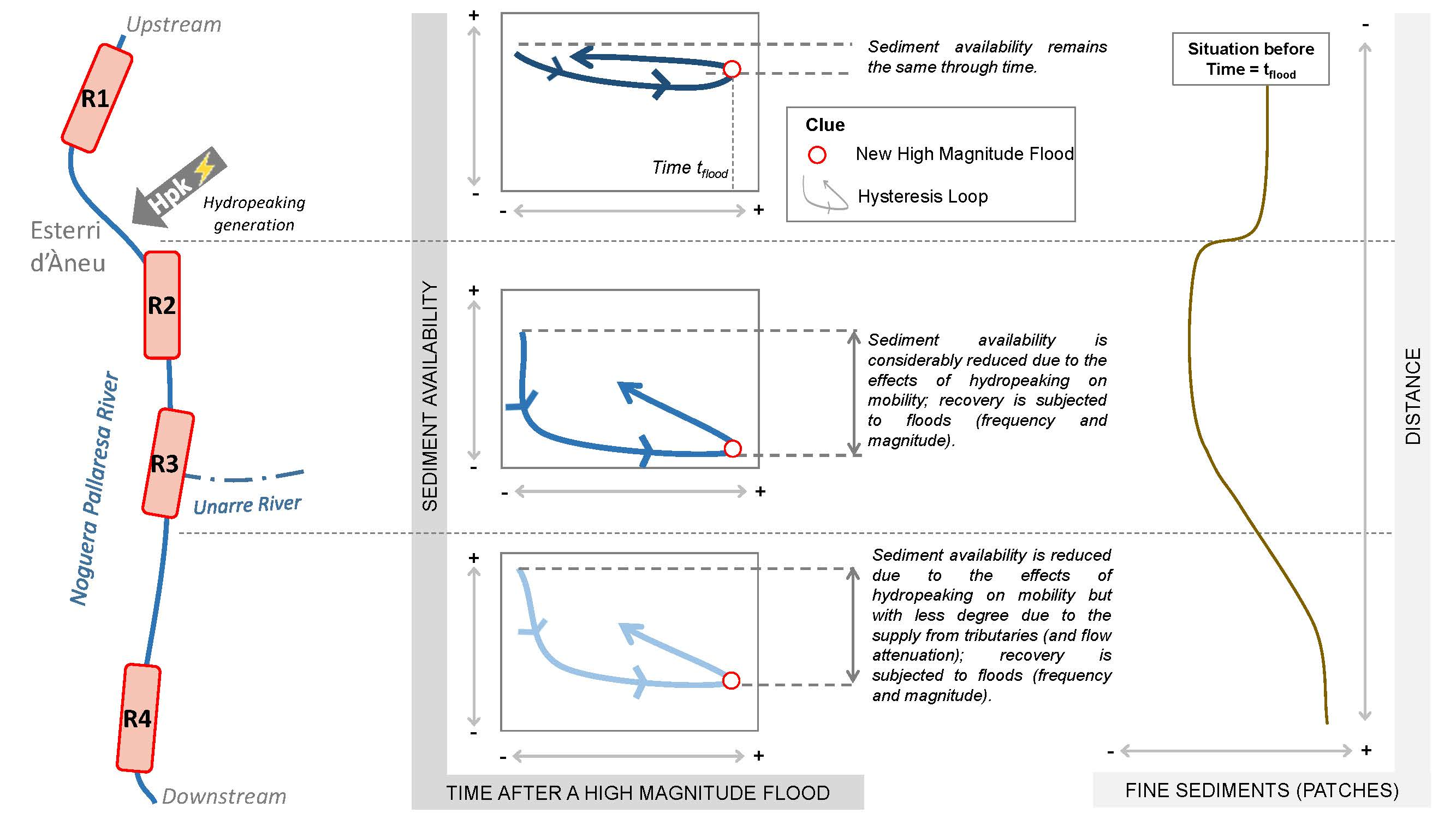
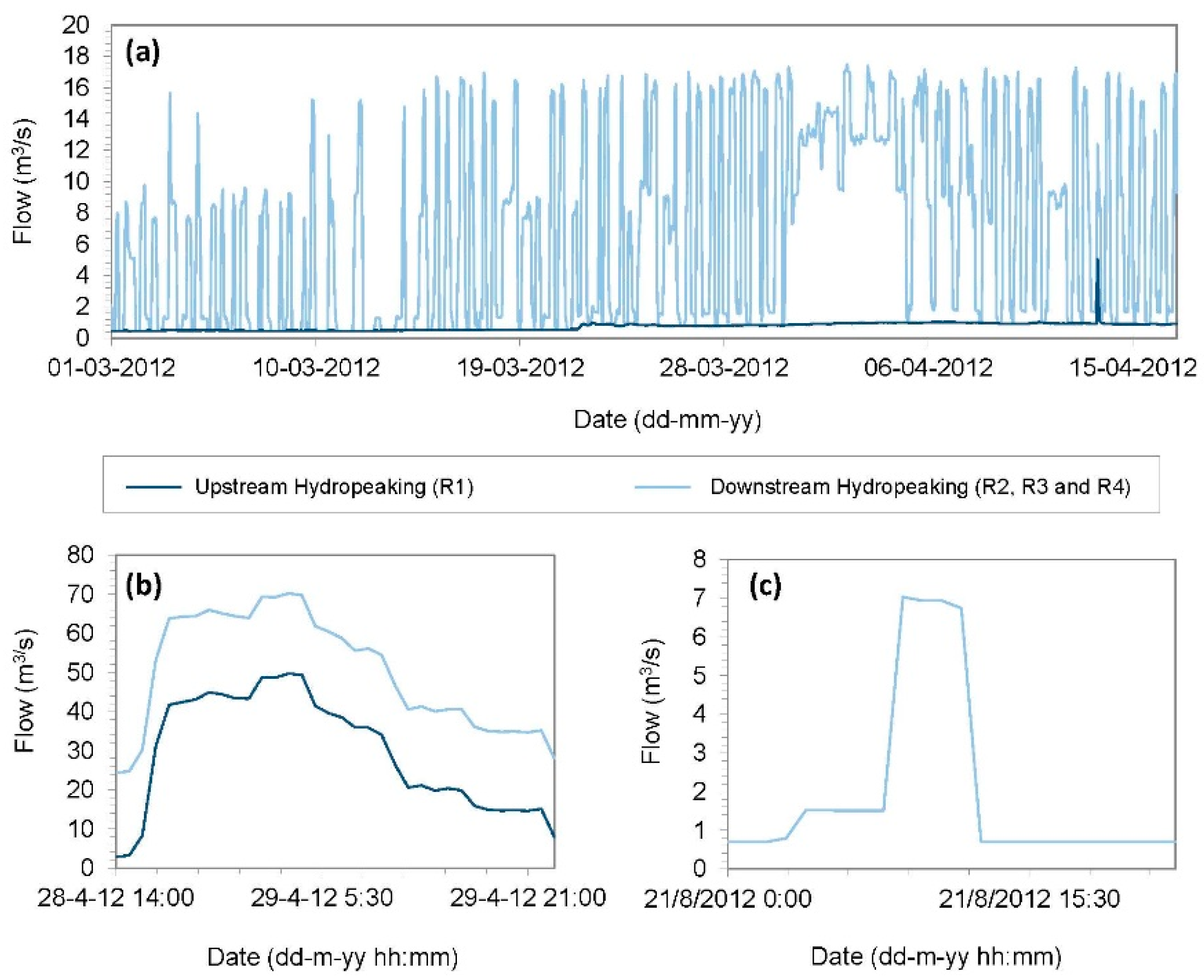
The catchment at the study segment (upstream La Torrasa Reservoir, Figure 1) has an area of approximately 330 km2. Upstream the study segment there is the Borén Reservoir (1 hm3 built in 1958), receiving a mean annual runoff of ca. 125 hm3. The Borén Reservoir stores and derives water to the Esterri-Unarre hydropower complex through a series of pipes and underground storage facilities (i.e., maximum generation capacity equates to 43 MW, whereas maximum discharge through turbines is around 23 m3/s) (see Figure 1b for location of the hydropeaking generation within the study reach). A discharge (Q) of 0.3 m3/s is released from the Borén Dam as environmental flow (i.e., Q95 of the flow duration curve). The hydrological regime is highly altered by the hydropower production; a typical hydropeak (Figure 2a) may attain ca. 20 m3/s and can occur twice a day. Flow duration curves display a median discharge (Q50) of 1.05 m³/s in the control reach upstream from the Hydropower Station (HP) where hydropeaks are generated, a discharge that increases to 4.06 m³/s in the downstream reach. Q90 and Q10 discharges are 0.49 m³/s and 2.66 m³/s in the control reach, and 1.73 m³/s and 16.52 m³/s in the impacted reach, respectively. Figure 2b illustrates the fluctuations of the daily Q observed downstream from the HP station. The station produces energy from a minimum of 4.1 h/day in August to a maximum of 23.8 h/day in May (information provided by the company in charge of the dams and the HP facilities, i.e., Empresa Nacional de Electricidad Sociedad Anónima (ENDESA).
The river displays a transitional morphology (i.e., step-pool to riffle-pool) in the reach upstream from the HP station (i.e., control reach), and a riffle pool configuration downstream from the station (i.e., impacted reach). Alternated bars are present during low flow conditions. Mean channel slope is 0.013 m/m and 0.007 m/m in the upstream and downstream reaches, respectively. River-bed-materials are composed by three well-differentiated sediment fractions (see Section 3.1 for more details): (i) The so-called structural materials mainly composed by large cobbles and boulders (D50 ranging from 880 mm in the control reach to 370 mm in the impacted reach); (ii) coarse movable particles mainly formed by gravels and cobbles with D50 ranging from 52 mm to 65 mm in both reaches, and (iii) patches of fine materials, mostly fine gravels and sand with a D50 of 1.9 mm in the control section and 0.8 mm in the impacted reach. The median size of subsurface materials ranges from 9 mm to 18 mm.
3. Methods
Four river reaches were monitored. One river is considered the control reach, located upstream from the HP station (i.e., R1, Figure 1), while the other three are located downstream (i.e., R2, R3, and R4, Figure 1b), being considered the impacted reaches. In the following sections we provide the details of methods used to survey channel topography and river-bed sediments, and characterise flow hydraulics and bed mobility.
3.1. Channel Topography
Topography was obtained to derive channel geometry and allow hydraulic modelling tasks (Figure 1). Topographic surveys started in December 2011 and were completed in February 2012. For this, a Leica VIVA® GS15 RTK-GPS (Heerbrugg, Sankt Gallen, Switzerland) has been used. A reference station was set up. The coordinates of this station were post-processed using the Receiver Independent Exchange Format (RINEX) data of the three closest permanent reference stations operated by the Institut Cartogràfic i Geològic de Catalunya (ICGC). Data post-processing was carried out using the Leica Geo Office® 7.0.1 software (Heerbrugg, Sankt Gallen, Switzerland). The 3d quality (positioning and height) of the final coordinates was 0.0086 m. The quality of the information surveyed with the mobile GPS unit was ca. 1 cm. In total, eight-hundred topographic observations were taken distributed through cross sections 10 m to 20 m spaced. A total of 24 cross-sections were surveyed together with a longitudinal profile for each of the reaches. The longitudinal profiles were used to calculate the averaged bed slope in each reach. The number of observations in each section varied depending on their topographic complexity. Water stage during surveys was obtained to support calibration and validation of the hydraulic model. The mobile GPS unit was also used to position photographs of bed sediments and to locate tracers during bed mobility experiments.
3.2. Flow Hydraulics and Hydrological Scenarios
Flow hydraulics were characterized by means of 1d modelling using HEC-RAS® (developed by the US Army Corps of Engineers, Davis, CA, USA). Modelled hydraulics were subsequently evaluated by means of direct field velocity measurements and continuous water depth data provided by a capacitive sensor (TruTrack WT-HR® (Christchurch, New Zealand) 1.5 m length) located in R1. Water depth was recorded every 15 min. A specific statistical relationship to transform water depth to discharge (h/Q) was derived. For each cross-section, the hydraulic conditions associated to peak flows of three different hydrological scenarios were modelled. These scenarios are fully characterised in the results section and further discussed, and are considered representative of the entire flow conditions in the control and impacted reaches. Specifically, Scenario 1 represents the combination of: (i) base flow conditions and low magnitude floods in the control reach (R1); and (ii) a series of highly frequent hydropeaks of similar magnitude in the impacted reaches (R2 to R4). Scenario 2 represents a high magnitude flood in both control and impacted reaches, together with the effects of hydropeaking and tributaries inflows in the impacted reaches. Finally, Scenario 3 represents an isolated hydropeak occurring in R2, R3, and R4. Flow data for each scenario were obtained by means of: (i) the water stage sensor located in R1; (ii) the flow data provided by the hydropower plant (data supplied by ENDESA); and (iii) the flow records available at the La Torrassa Reservoir (data supplied by ENDESA), which is located further downstream (see Figure 1 for location details).
3.3. Bed Materials Characterization
3.3.1. Surface Materials
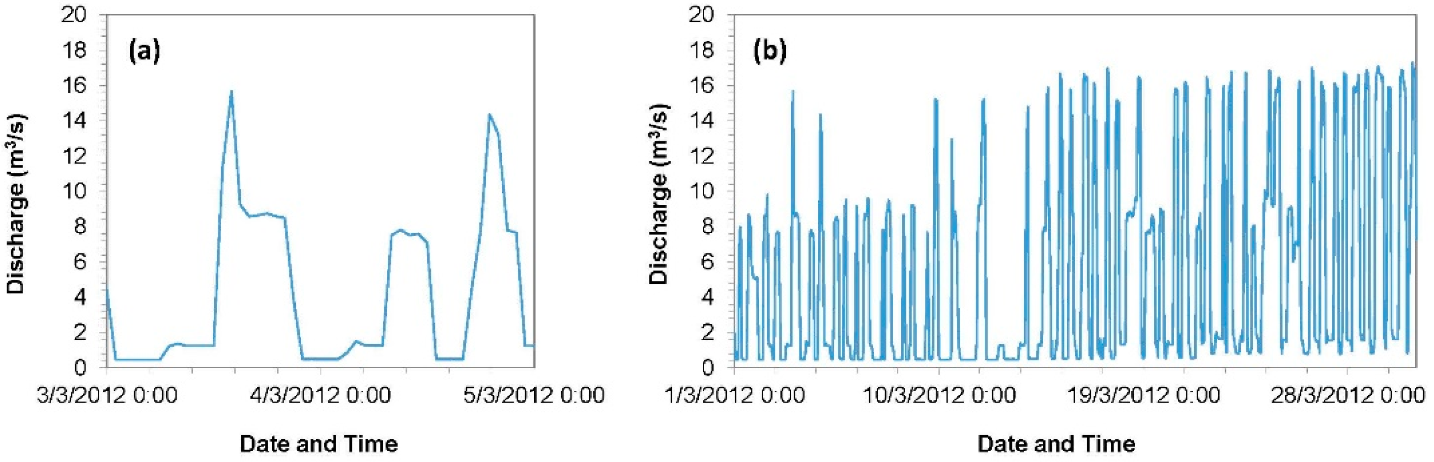
River-bed materials are composed of three well-differentiated sediment fractions, which have a direct effect on the mobility patterns observed in the channel: (i) structural materials (Figure 3a), (ii) coarse movable particles (Figure 3b), and (iii) patches of fine materials (Figure 3c). The methodological design for the characterization of the bed materials was based on these observed components. The grain-size characterization of the surface materials was carried out in two phases. Phase I assessed the proportion of the three sediment fractions in each of the study reaches, while Phase II undertook the characterization of the grain-sizes properly.
For Phase I, a variant of the pebble count method [30] was used, with the objective of quantifying the proportion of each of the three fractions over a total of 100 measuring points distributed along linear transects in each reach. The type of material (i.e., structural, coarse or patch) sitting in each observational point was annotated, so the percentage of each component was assessed. Particle sizes were then characterized (Phase II). The two coarser grain-size fractions (structural materials and coarse surface layer, see Figure 3a,b) were measured following the pebble count method [30,31]. Particles were classified (b-axis) by passing them through a template divided into ½ Φ size intervals (e.g., [32]). The b-axis of the structural sediments was obtained by means of a ruler. The classification of the sediments was based on the Wentworth scale (where Φi = −log2D, being D the size of the particles in meters). In total, 450 particles were measured.
For the characterization of the fine surface sediments that form the patches, a photographic method was used. The photographic method represents an indirect method to obtain Grain-Size Distributions (GSD), allowing for the characterization of sedimentary units without modifying their structure. The photographs were analysed using the Digital Gravelometer® (University of Loughborough, Leicestershire, UK). This software allows the rectification of the photographs through knowing the distance between control points (i.e., the real length between points identified in the photos), the identification of particles and the automatic calculation of the length of the axes of these. GSD resulted from the two methods, in which the particle’s b-axis and their accumulated frequency are displayed, allowing the extraction of characteristic grain-size percentiles such as the median particle size (D50), the D84 and the D16.
3.3.2. Subsurface Materials
Subsurface materials were sampled in two of the four reaches (i.e., R2 and R4; see Figure 1 for location). The spatial variability of subsurface materials can be considered small among relatively localized reaches. Sediments were characterized by means of the volumetric method after extraction of the surface layer in exposed bars during low flows. An area of 1 m2 was delimited and painted with quick-drying spray paint; painted particles were removed, exposing the underneath subsurface materials. For the determination of the total volume of the sample, it was considered that the largest subsurface particle (Dmax) did not exceed 3% of the total weight of the sample [33], a criterion that is considered adequate when the median of the material to be characterized is located in the fractions of coarse gravels and pebbles. The b-axis of the Dmax ranged between 75 mm and 100 mm. The largest fractions were sieved in the field while the finer were processed in the laboratory. As in the case of surface material, the sieves followed ½ Φ intervals. A total of 60 kg of material were processed. Once sieved, a grain-size curve for each sample was plotted. The comparison of the medians (i.e., D50) of the surface and subsurface GSD permits quantification of the degree of armouring [34]. When the ratio is >1.5, it is considered that there is a marked difference between the surface and the subsurface materials, while when the ratio approaches to 2 indicates incipient armouring. Higher ratios correspond to well armoured structures, often induced and controlled by sedimentary imbalances such as those occurring downstream from dams (e.g., [4]).
3.4. Bed-Material Mobility
3.4.1. Mobility
Bed-material mobility was studied by means of tracer stones (e.g., [35,36,37,38]). The objective was to determine the size, the distance and the trajectory of displacement of traced sediments after each of the monitored flow scenarios. Although there are different methods, we traced sediments by means of painting (e.g., the origin of the tracer is available based on the colour of the paint) and by means of passive sensors (or tags), in our case Radio Frequency Identification (RFID).
Painted particles (Figure 4) allow tracking their movement by re-surveying their position once competent flows entrain and displace them. Their position is obtained by means of the RTK-GPS (see Section 3.1 for details). The size of the particles was also measured. This method is simple but it allows for the tracing of many particles at a time, which is important to have a representative sample of the bed material. Although particles can be traced independently (one by one), a complementary alternative to the method is to paint small areas of the bed (e.g., around 1 m2). This method does not allow sediment tracing in the active (wet) channel but, conversely, allows sediment to be traced without modification of the sedimentary structure of the bed (exposed bars). This is important in rivers with high grain-size complexity where imbrication and surface compaction, together with the presence of sedimentary structures, can control the conditions of the onset of movement, as is the case of the Noguera Pallaresa. In this case, the initial location of the painted particles is considered at the centroid of the painted square. While this yields an uncertainty in the real initial position of each of the painted pebble recovered after a competent flow event; yet, when mobility is relatively high (meters), the uncertainty is compensated for by the large number of pebbles traced and recovered.
The recovery rate associated with painted pebbles is relatively low (<50%), but the high number of traced particles allows obtaining representative data. In our case, this method has been applied to the coarse movable particles and to the patches of fine materials exposed in dry areas during low flow conditions. The method has proven useful to observe the mobilization of relatively fine sediments, materials of great importance for the habitat (fine gravels and sand) that, due to their size, cannot be traced by means of RFID. The average grain-size (b-axis) of the painted tracers found after mobility ranged between 9.4 mm and 18.2 mm.
Larger particles were marked by means of ‘passive’ (i.e., do not need battery and are activated only when they are detected from a mobile receiver or antenna) RFID tags (Figure 5). These type of sensors contain antennas to respond to radiofrequency requests, allowing to register the RFID code once it is detected, which is unique per each particle. The size of the RFID tags is a limiting factor since they have to be introduced and sealed inside the particles. In this study, 22-mm and 32-mm sensors were used, which limited their applicability to sediments with b-axis smaller than 50 mm (i.e., coarse gravels). These tracers can be used in the active channel and the recovery rate may attain >80%. In our case, a total of 65 tracers between 48 mm and 174 mm of the b-axis were in two of the study reaches. The mean particle diameter was 94.5 mm in R1 (n = 33) and 90.5 mm in R2 (n = 32).
3.4.2. Entrainment Conditions
Theoretical or predicted critical shear stress for selected particle sizes was calculated using the Shield’s Equation:
where τc is the theoretical critical shear stress (N/m2) for a particle size D, ρ’ is the submerged sediment density (kg/m3), g is the acceleration to gravity (9.8 m/s2) and τc* is the dimensionless shear stress (or Shield’s number) modified for gravel mixtures (0.045, as suggested by Church [5]).
τc = τc*Dρ’g
We have considered the observed critical shear stress for a given particle as the value obtained in each reach based on: (i) the largest mobilised particle size; and (ii) the average water depth associated to the peak flow for the given mobility period (i.e., time between surveys). Water depth and shear stress values were obtained from the 1d modelling, based on the DuBoys equation.
Additionally, the specific stream power associated to the peak discharge of each scenario was calculated using the following Equation:
where ω is the specific stream power (W/m2), ρ is the water density (kg/m3), Q is the peak discharge (m3/s) and w is the channel width (m).
ω = ( ρgSQ)/w
4. Results
4.1. River-Bed Topography and Grain-Size
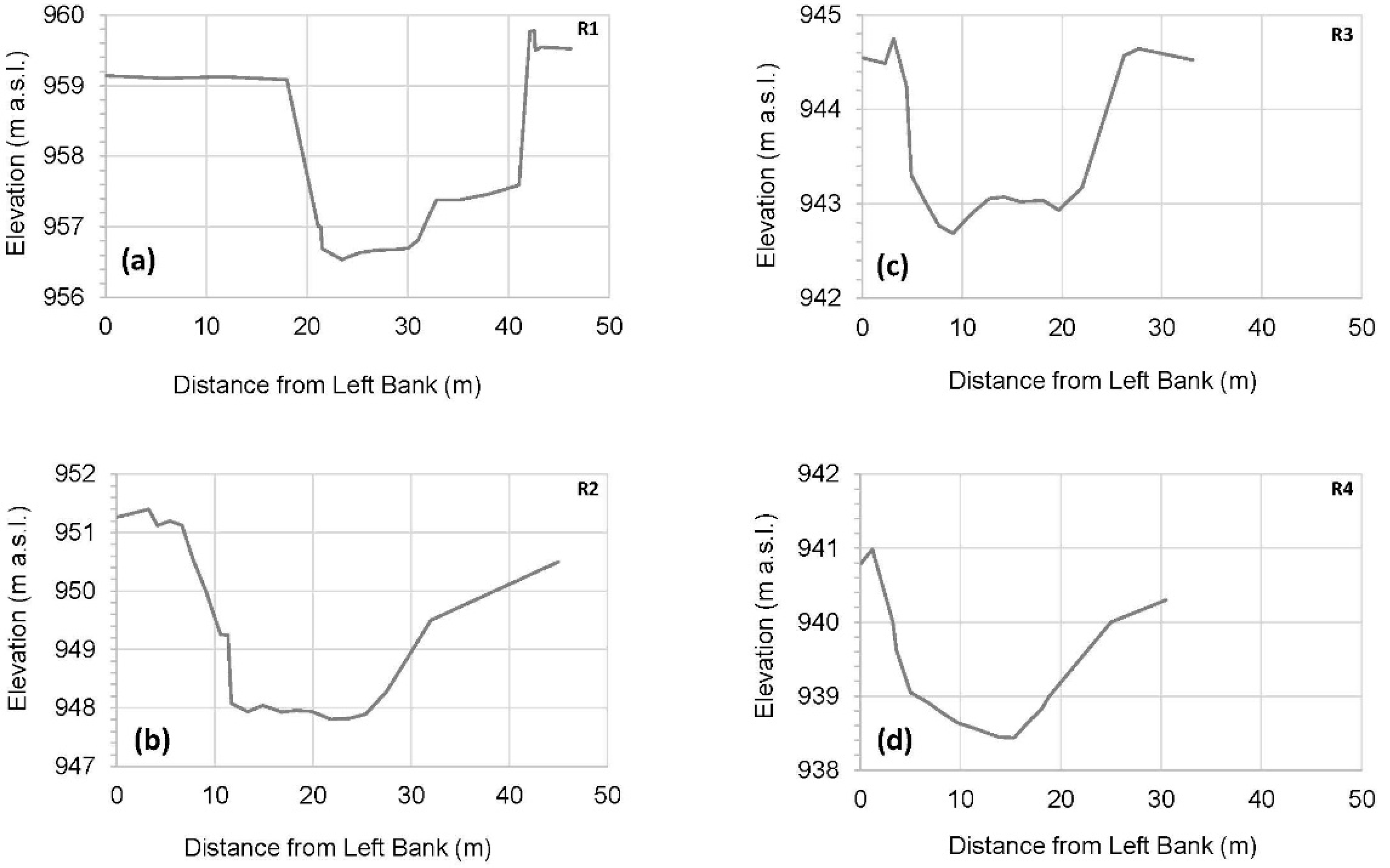
Channel geometry was similar in all of the study reaches (Figure 6). Mean wet channel width associated with the median discharge (Q50) was around 10 m, with mean water depth ranging between 0.11 m and 0.20 m. Channel geometry in R1 and R2 is constrained by a series of embankments of around 2 m high (above the thalweg), determining that, during flood events, an increase in Q is mainly controlled by an increase in depth and velocity. However, these embankments do not affect any of the hydraulic and sediment transport analyses presented in this manuscript due to the length of the active channel width in relation to the studied flows. Mean slope in R1 is 0.013 m/m, while downstream it reduced to 0.008 (R2), 0.007 (R3) and 0.006 m/m (R4). These differences have a direct influence on flow competence. For the same Q, and taking into account the similar channel geometry observed in all reaches, the higher slope in R1 provided larger shear stress. However, and as discussed below, higher shear stresses do not necessarily mean greater mobility, since this is ultimately controlled by the size of the particles and the local river-bed structure.
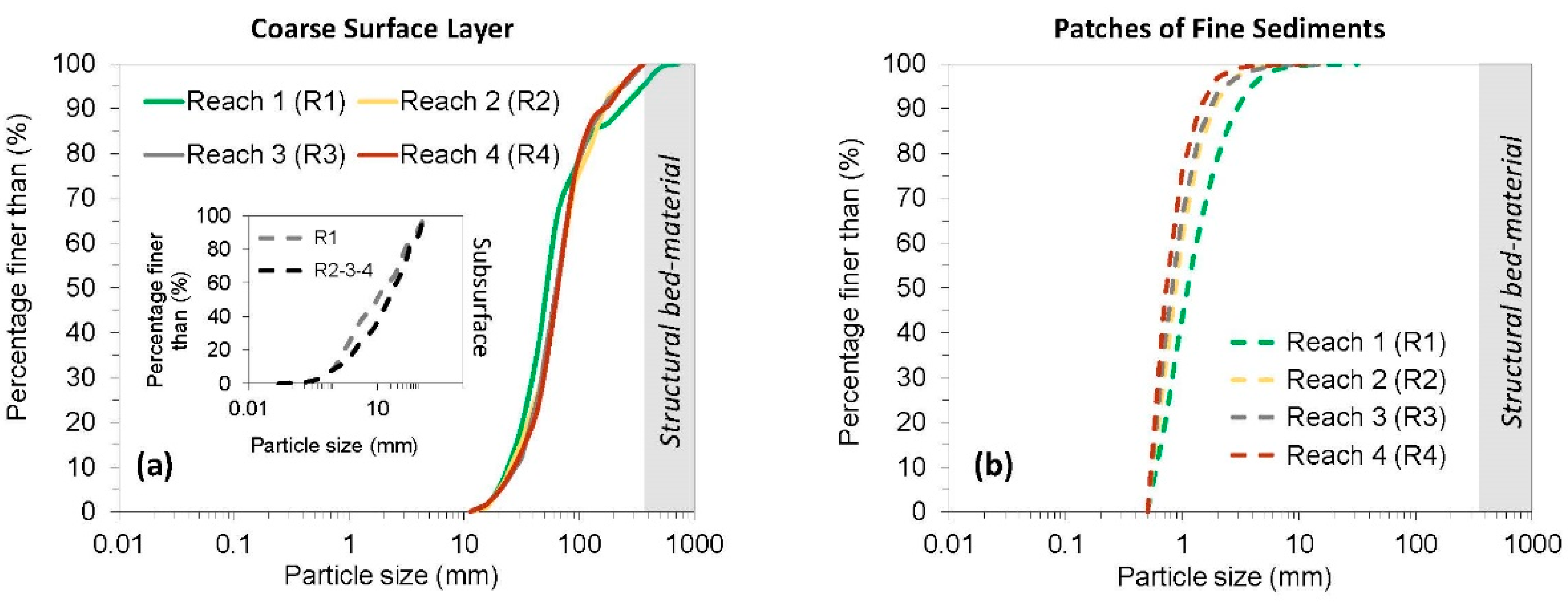
Table 1 shows a summary of the river-bed grain-size values obtained in each study reach, while Figure 7 shows their respective GSD. The proportion of Structural surface materials, Coarse movable surface materials and Patches of surface fine materials varied between reaches. The reach presenting more structural materials was R1 (15%), while the presence of these elements in R3 and R4 was marginal (ca. 5%). The size of the structural elements ranged between 881 mm in R1 and 373 mm in R4. These particles have limited mobility but play an important role on channel hydraulics and mobility of finer materials, mainly through hiding and protrusion (e.g., [13]). The percentage of fine materials in patches oscillated between 12% (in R2) and 22% (in R4), although the proportion was variable through time associated to hydropeaking and sediment supply from upstream and from tributaries, as discussed below. The size of these materials was similar, all in the range of coarse sands and fine gravels (around 1–2 mm). The majority of the bed was covered by coarse-mobile surface materials (between the 67% and 78% of the bed). Median sizes were in the range of coarse gravels, with moderate to poorly sorted distributions as indicated by the sorting [39] values (Table 1).
Two subsurface samples of the bed material were obtained, one in R1, representing the control reach, and another one in R3, a reach impacted by hydropeaking. Median subsurface particles were in the range of median to coarse gravels. Although both GSDs are very poorly sorted, there is slight difference in terms of the median particle size (Table 1). In general, the river-bed is armoured, although armouring in R1 is clearly higher than the one obtained for the hydropeaked reaches.
4.2. Flow Scenarios
Flow hydraulics and associated bed mobility were analysed based on the three different flow scenarios, taken as representative of the entire flow conditions in the control and impacted reaches (Figure 8) during the study period.
4.2.1. Scenario 1
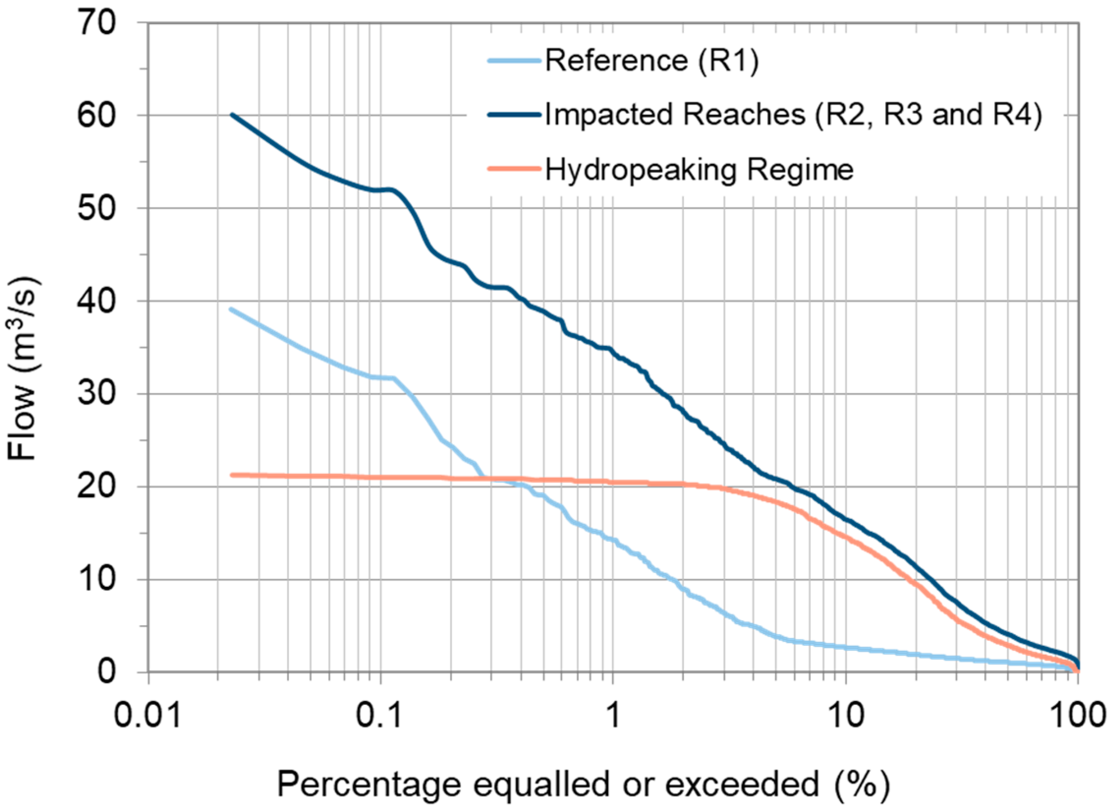
The specific period under this scenario was 1 March to 18 April 2012 (Figure 8a). The mean Q in R1 was around 0.7 m3/s, while the peak flow of the unique flood registered in this section was ca. 5 m3/s. The mean daily Q during the flood was 1.2 m3/s. This value corresponds to a flow equalled or exceeded the 41% of the time (Figure 9). Shear stress associated with the peak flow was 48 N/m2 while the specific stream power was 46 W/m2 (see flows in Table 2 and specific stream power values in Table 3). Downstream, in R2, R3 and R4, flows were significantly different in comparison to R1 due to the effect of the hydropeaks (Figure 8a). Hourly Q ranged between 0.5 m3/s and 17 m3/s (average flow of 7 m3/s). Maximum daily flow was 13.9 m3/s and it was equalled or exceeded the 15% of the time (Figure 9). Shear stress associated with the maximum Q ranged between 33 N/m2 (R4) and 42 N/m2 (R2); specific stream power oscillated between 67 W/m2 and 88 W/m2 (Table 2 and Table 3). Flow differences between the control and impacted reaches were evident. These differences are not directly translated to shear stress. This fact is mainly due to the role of the channel gradient on the shear stress computation. Differences are, however, evident in terms of stream power. The persistence of characteristic Q values in each reach was highly distinct, i.e., whereas in R1, the peak Q (5 m3/s) constituted a single observation during the whole period, peak values around 17 m3/s were observed daily in the downstream reaches (Figure 8a). Differences in the magnitude and frequency of the hydraulic conditions had a direct impact on bed mobility and, subsequently, on physical habitat availability.
4.2.2. Scenario 2
The period analysed in this scenario encompassed 28 to 29 April 2012 (Figure 8b). The maximum Q registered in R1 was around 50 m3/s, yielding an average daily Q of 30 m3/s. This value was equalled or exceeded the 0.1% of the time (according to the flow duration curve of the river; Figure 9). Therefore, it can be considered a high magnitude flood. Shear stress associated to the peak flow in R1 was 124 N/m2, while the specific stream power was 303 W/m2 (Table 2 and Table 3). R2, R3, and R4 experienced the additive effect of hydropeaking and tributaries, increasing the peak Q to 70 m3/s, yielding a mean daily Q of ca. 50 m3/s, again equalled or exceeded the 0.1% of the time (Figure 9). Shear stress in the impacted reach R2 attained 99 N/m2. Differences in the specific stream power between R1 and R2 were insignificant (Table 3).
4.2.3. Scenario 3
In this case only the conditions associated with hydropeaking were analysed and, consequently, only R2, R3 and R4 reaches are considered (Figure 8c). Note that no mobility was observed in R4 during this scenario. The studied hydropeak was registered on 21st August 2012. Maximum Q was ca. 7 m3/s, significantly smaller than the maximum Q that the HP station can generate (i.e., 23 m3/s). Differences in terms of shear stress and specific stream power between reaches were minimum (Table 2 and Table 3). The mean Q of the hydropeak was 1.9 m3/s (Figure 8c), equalled or exceeded the 63% of the time (Figure 9). This mean value is equalled or exceeded the 85% of time in the impacted flow duration curve (Figure 9). The high frequency of these flows (more than the magnitude) plays an important role on particle mobility and in-channel sediment depletion.
4.3. Bed-Material Mobility
Bed mobility in the control and impacted reaches was assessed through the analyses of (i) particles entrained and (ii) the entrainment thresholds under each of the flow scenarios.
4.3.1. Field Observations
The size and step-length of the entrained particles was remarkably different between scenarios and reaches. A summary of the bed mobility observations is presented in Table 2. Table 3 presents the largest particle size mobilized in each scenario and the shear stress and specific stream power associated to each analysed peak flow.
Scenario 1
Only the small fractions of the coarse-mobile GSD were entrained in R1. The mean size of the entrained particles was 1 mm, while the largest entrained particle was 31 mm (Table 2), smaller than the surface D16 (movable component). The results indicate that the relatively small peak flood in the control section (5 m3/s) were sufficient to entrain coarse sands and fine gravels from the patches. Although the flow was competent, step length was marginal (lower than 0.5 m). Further downstream, in the impacted reaches (R2 to R4), mobility patterns were substantially different to those observed in the control section. Maximum Q was more than threefold larger, with daily oscillations. The size of the entrained particles increased; the largest entrained particles ranged between 38 mm and 42 mm (i.e., larger than the D20), while the mean of the mobilised sizes varied between 13 mm and 21 mm (Table 2). The step-length was very variable, probably attributed to the complexity of the surface materials and the hiding and protrusion effects of the immobile particles. Figure 10 shows the GSD of the recovered tracers together with their step-length. The largest step length was ca. 6 m (observed in R2). Overall, the data show that the hydropeaks were capable of entraining the full range of the fine particles of the patches and the finer ~30% of the GSD for the coarse movable fraction of the bed material. Structural elements did not move in any of the study reaches. Overall, mobility analysis in this scenario indicates a size-selective pattern associated with the distinct hydraulic conditions (both in terms of frequency and magnitude) observed in the control and impacted reaches.
Scenario 2
Only data in R1 and R2 were obtained under this scenario, which are representative of the both control and impacted reaches. Large floods were able to entrain the full range of coarse-mobile particles in both reaches. The largest entrained particle in R1 was 171 mm, larger than the D84 of the movable component. Similar competence (i.e., particle calibre) was observed in the impacted reach, but particles were transported further downstream (1.5 times more) in comparison to the control reach (Figure 10). This fact may be attributed to the additive hydraulic impact of the hydropeaks, as can be seen in Figure 8b (Table 2). The step-length was not, however, clearly controlled by the size of the particles, as was evident in the scenario 1. In general, the results indicated that high magnitude flood events were able to entrain the totality of the mobile components of the river-bed materials (i.e., full mobility conditions) in both the control and the impacted reaches.
Scenario 3
The effects of an isolated low magnitude hydropeak were also analysed. Entrainment was only observed in R2 and R3, no mobility was seen in R4. Results for this scenario are similar to the ones observed under scenario 1, although differences between reaches are more significant. In general, mobility was higher in R3 than in R2. The largest entrained particles in R3 was one order of magnitude higher than in R2 (7 vs. 62 mm, Table 2). These values encompass all the size range found in the patches and up to the D50 of the coarse movable component in the case of R3. Differences are smaller when the average entrained particle sizes are compared. The mean and largest step length in R2 were similar, i.e., around 1.5 m (Figure 10). As in scenario 1, patterns observed in R3 indicated that the range of particle sizes having short displacements was large when compared to the one associated to the largest step-lengths. Particles were displaced further in R3; 2.6 m on average with a maximum step-length of around 7 m. These observations highlight the importance of sediment availability during hydropeaking.
4.3.2. Entrainment Thresholds
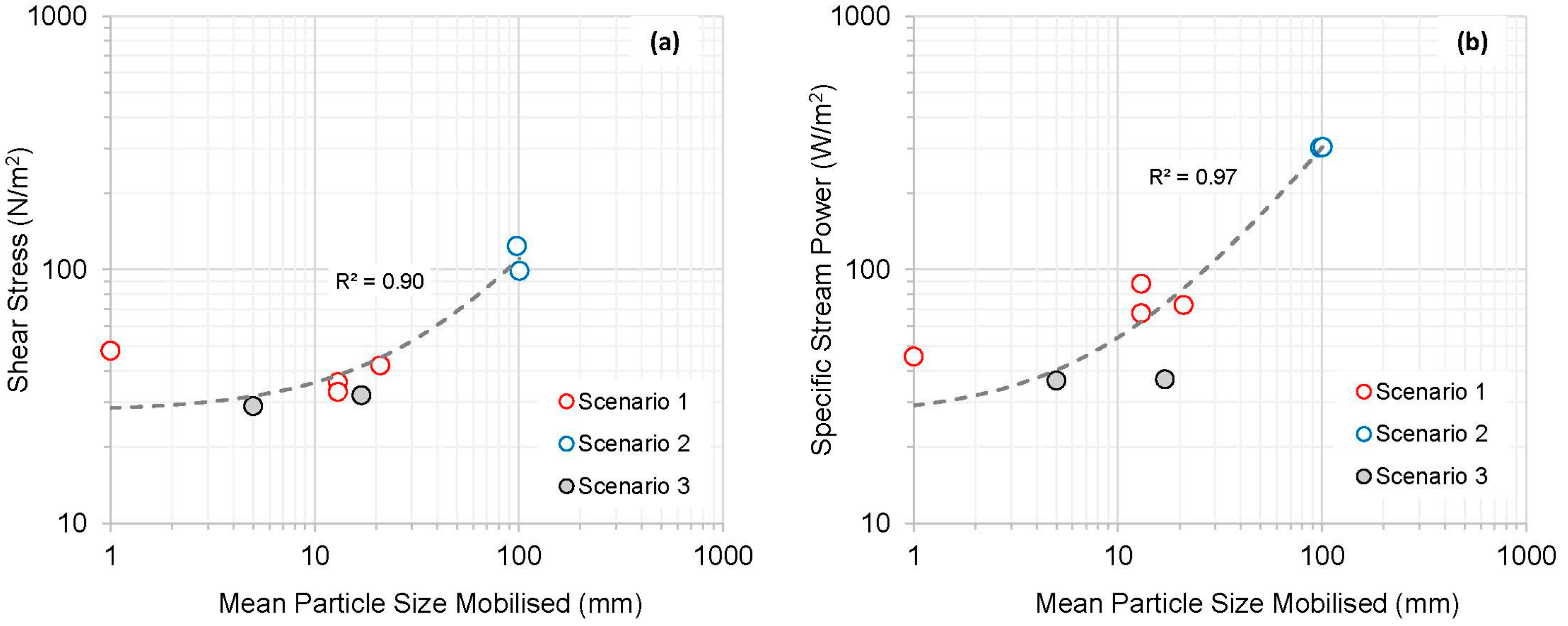
Figure 11 shows a relation linking critical shear stress and specific stream power to the mean particle size mobilised (i.e., the mean b-axis of the recovered particles). Although the small number of observations, results indicate that exists a general positive relationship between the stress generated by the flow and the mean particle size mobilised under the different hydrological scenarios. In terms of minimum shear stress, mobility was observed around 32 N/m2, while in terms of stream power, a minimum of 37 W/m2 are required to entrain the mobile components of the substrate along the entire study segment. These values were observed in R3 during the ‘A single hydropeak’ scenario (i.e., S3). The largest values of stress and specific stream power were observed during the high magnitude flood event (i.e., S2). Although both lineal models fitted to the data present a high coefficient of determination, it is clear that the one for the specific stream power is higher. These differences may be attributed to the way both variables are calculated. In the case of the shear stress, the values are calculated by means of the DuBoys approach, while the characteristics of the flows and the channel may not be the appropriate as will be extended below. Data observed in Figure 11b fits above the majority of the published relations linking critical unit stream power to the size of material in gravel-bed rivers (e.g., [40]). These differences may be attributed to the hiding effects caused by the structural large elements in the bed, as suggested by the high variability of the magnitude of the step-lengths observed, which is probably due to the complexity of the surface materials which may, in turn, delay the entrainment of the particles in the study segment.
Theoretical critical shear stress for the largest particles mobilised in each scenario was assessed following the Shields’s approach. Results were compared to the shear stress associated to the peak Q of each scenario estimated by means of the DuBoys approach (based on the 1d modelling results, mean values). Table 4 summarizes both entrainment thresholds. Additionally, it also shows the predicted values of critical shear stress for representative percentiles of the coarse component of the GSD.
Results indicate that theoretical thresholds are underestimated when compared to the observed critical shear stress needed to entrain the largest particle sizes mobilised in R2 and R3 (see residuals in Table 4). Results in R1 and R4, however, indicated an agreement between both observed and predicted thresholds. Even so, when the full spectrum for mobilised particles are analysed, the results indicate that theoretical thresholds tend to be underestimated. For instance, theoretical critical shear stress for particles between 29 mm and 35 mm ranges from 21 N/m2 to 25 N/m2, while field observations associated to scenario 1 indicate that the critical shear stress to entrain particles between 31 mm and 42 mm ranged from 33 N/m2 to 48 N/m2.
5. Discussion
5.1. Spatial and Temporal Effects of Hydropeaking on River-Bed Mobility
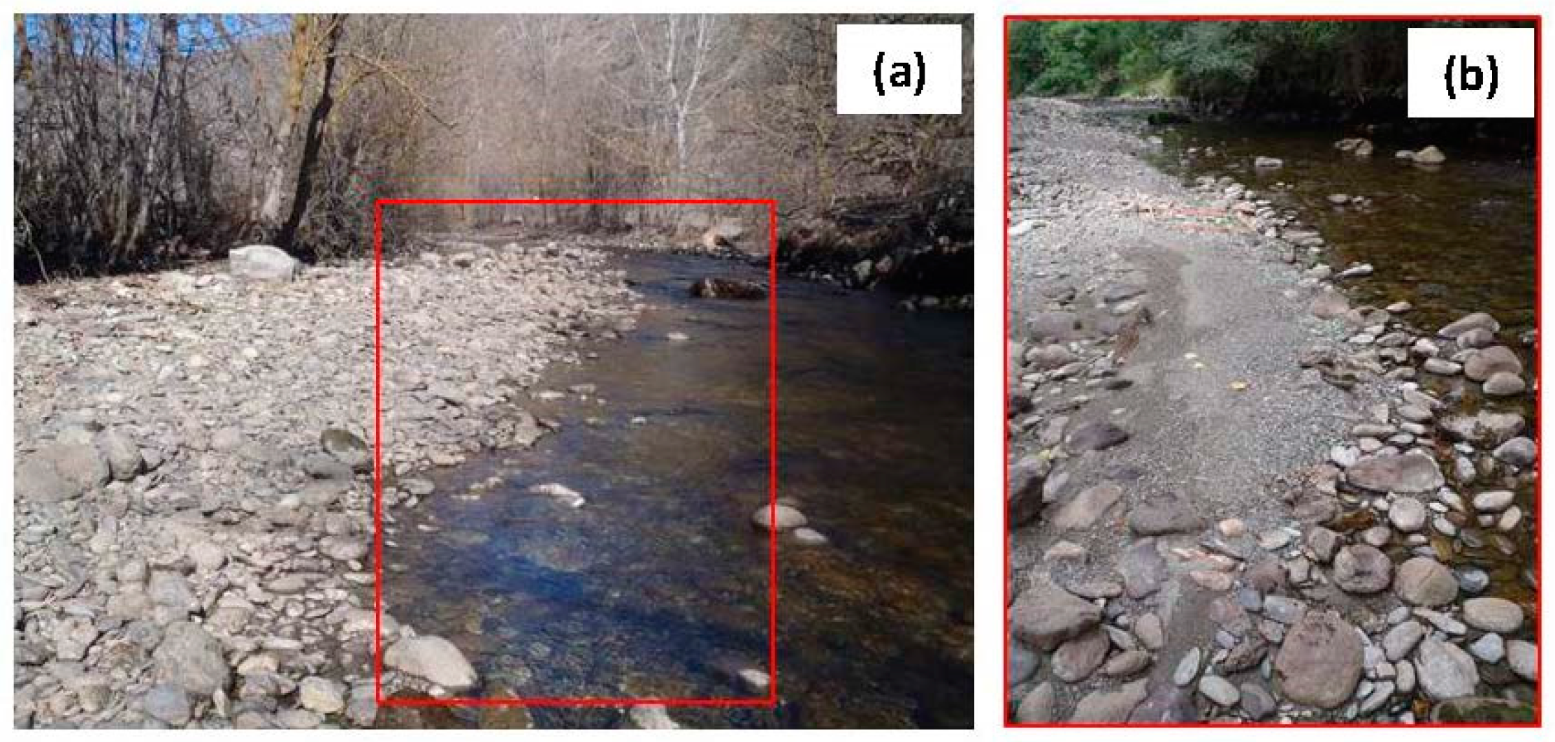
Our results indicated as the effects of hydropeaking on mobility are not observed for the whole spectrum of grain-sizes present in the river-bed. These are also controlled by sediment availability, mainly those sizes present in the coarse mobile component of the substrate and in the patches of fine materials. In the absence of relatively large floods only the sediment supplied from tributaries during small flood events may reduce the effects of hydropeaks on river-bed particles’ availability. Figure 12 shows a close-range picture of R3 in two different periods illustrating the differences in sediment availability which in this reach is controlled by the sediment supply from the River Unarre (see Figure 1 for location details). The figure also shows that the bed armour was not strong. These facts are key to understand the differences in mobility between reaches. Further downstream, field observations pointed out that the presence of fine sediments (fine gravels) in R4 was much lower than in R3. This fact may suggest a delay in the transfer of this type of materials from the Unarre by the time the mobility episode was analysed. In summary, our results pointed out that single hydropeaks, even of reduced magnitude, have enough competence to entrain an important part of the river-bed materials i.e., all sediments range from patches and a significant proportion of the coarse movable surface materials. Mobility is spatially variable in relation to local sediment availability and flow hydraulics. Sediment availability changes through time in relation to sediment supply from upstream and tributaries, mainly during flood events.
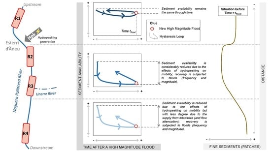
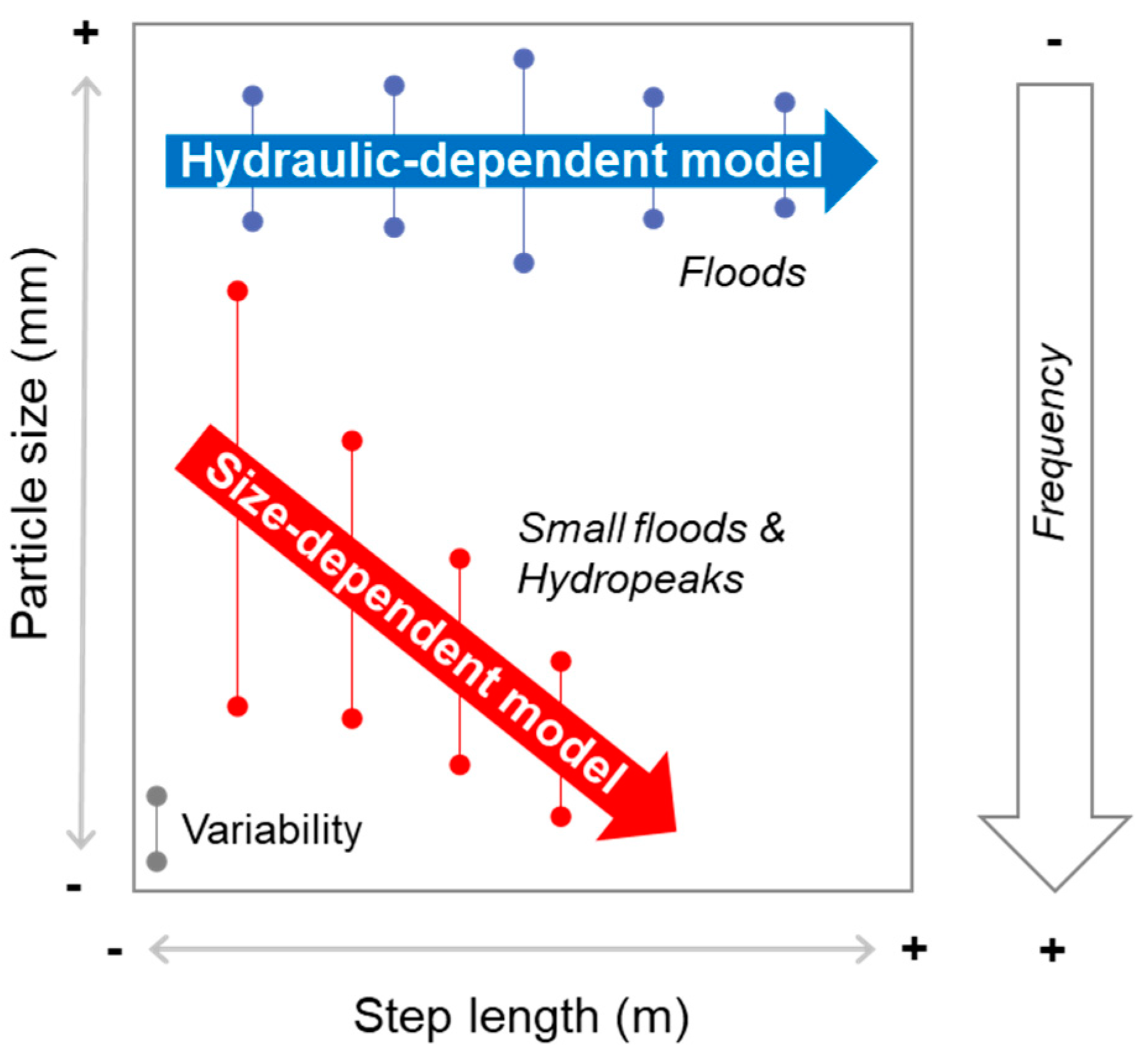
Results from this study indicate that hydropeaked rivers may be subjected to two general bed mobility models (Figure 13):
- (a)
- Size-dependent model in which the displacement of sediments is inverse to their size. This model can be attributed to low magnitude floods and to the entire hydropeaking regime, mainly affecting fine surface sediments (typically from patches) and the finer part of the coarse movable GSD. Flow hydraulics during these conditions are of low magnitude and high frequency and are not competent to entrain and transport the entire spectrum of the surface bed materials (mobile fractions). This model is also conditioned by sediment availability, a fact of great importance in the hydropeaked reaches where the frequency of these flows is daily and the entrainment of bed materials is not balanced by the supply of sediment from upstream. Under these conditions the river-bed becomes depleted of fine sediments from patches (e.g., [14]) and progressively lacks other fractions such as medium gravels, all of which are highly relevant from an ecological point of view. These reaches can be classed as supply-limited, as their incipient sedimentary recovery can be observed downstream from tributaries (as the Unarre in our study case) that periodically supplies fresh new sediments to the mainstem Noguera Pallaresa, and also due to the loss of competence of hydropeaks as they are routed downstream.
- (b)
- ‘Hydraulic-dependent mobility model’ in which the displacement of particles is not conditioned by their size, but depends on the magnitude and duration of a given competent flow. This model is generally linked to high magnitude floods that exhibit the capacity to mobilize most of the mobile sediments in the channel, i.e., all except the structural elements. The frequency of these flows is relatively low but they determine the supply of sediment to both the control and impacted reaches. High competence may cause the break-up of the armour layer (see for instance examples in dammed rivers e.g., [12]), supplying fine subsurface sediments and, together with the overall sediment supply from upstream, increasing their availability along the river channel. The frequency of these flows also influences the mobility observed during hydropeaking, a fact that is again related to the availability of sediment in the river bed (Figure 13).
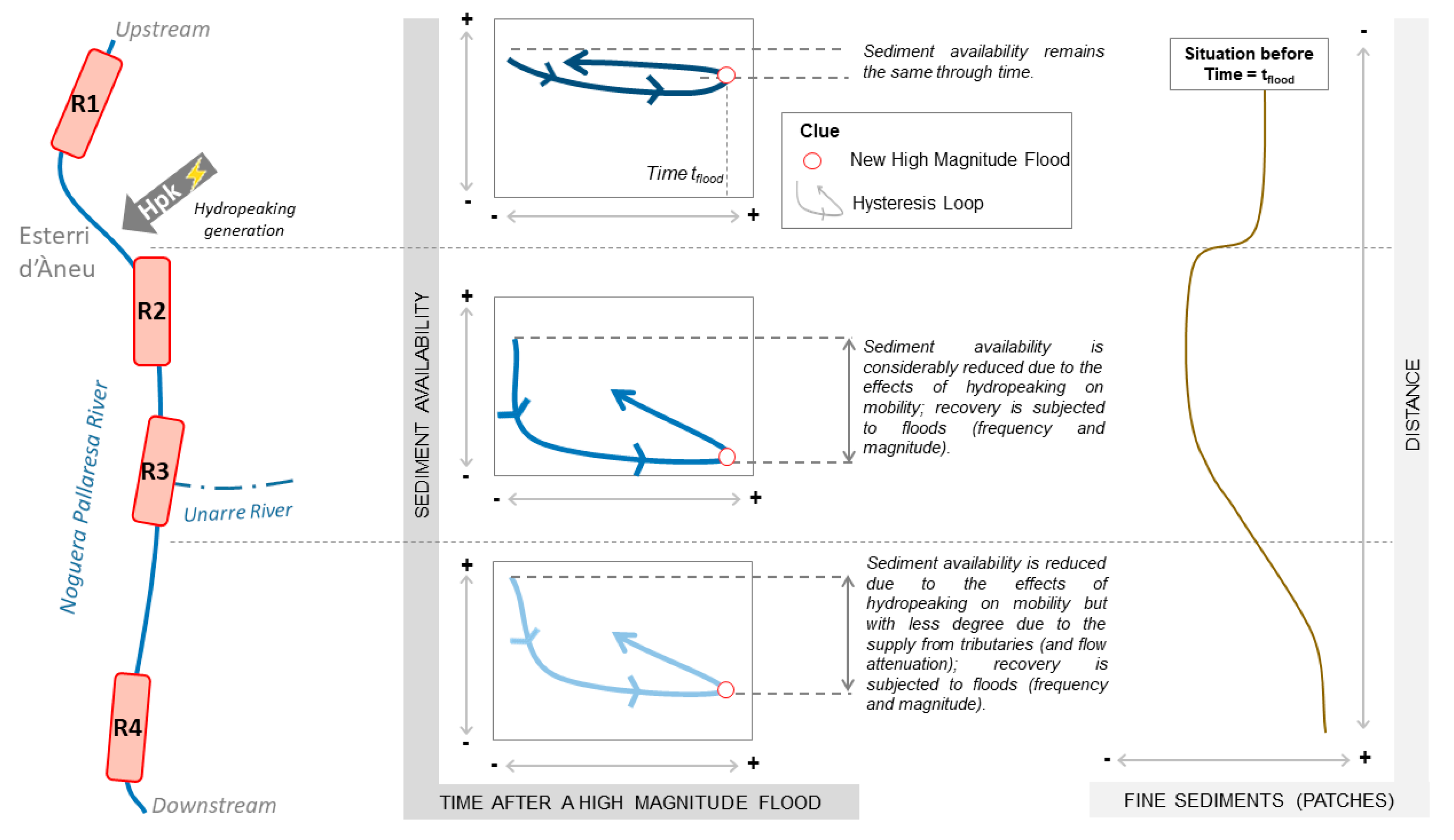
The combination of these two mobility models generates counter-clockwise hysteresis cycles in the availability of fine sediments (sand and gravels) in relation to the time elapsed since the last high magnitude event occurred (Figure 14). These cycles occur mainly in reaches subjected to hydropeaking. Sediment availability in non-hydropeaked reaches is determined by the balance between the supply of sediment from upstream and the export during competent events. There is therefore an upstream transfer and continuity in sediment transport and in-channel sediment availability does not change significantly if a flood event does not occur (Figure 14). In contrast, conditions are different in the hydropeaked reaches where flows are altered daily, often reaching critical conditions to entrain fine sediments from the bed. As explained above, those flows yield a size-dependent model, in which fine sediments are entrained without replacement from upstream (and eventually depleted), while larger materials (e.g., coarse gravels) remain relatively immobile. The size of the loop of the hysteresis is inverse to the distance from the point where the hydropeaks are generated. Close to the hydropower station in R2, sediment availability reduces significantly and relatively rapidly (related to the frequency of competent hydropeaks). Further downstream, these processes are mostly modulated by tributaries which periodically supply sediments and flow to the mainstem river (e.g., Figure 12). In the particular case of our study, flow hydraulics and hence flow competence, does not change substantially downstream, therefore the role of the tributary is highly relevant. Once a high magnitude flood occurs hydraulically-dependent bed-mobility dynamics takes place and a new situation of sediment availability was generated to all reaches (i.e., dashed lines in Figure 14). The direction of change is variable and it will be determined by the amount of sediment supplied from upstream and the flow competence and capacity, which varies in time and space.
5.2. Bed Mobility and Habitat
Results from this work indicate that hydropeaks enhance the mobility of the relatively fine fraction of the river-bed sediment that becomes depleted until a natural flood re-supplies the reach and sediment becomes newly available. Sediment entrainment and depletion form patches of fine materials have been reported before, often attributed to the early stages of floods or during low magnitude events in which flow competence is limited (e.g., [41]). Vericat et al. [14] reported that depletion of fine sediments from patches in gravel beds occurs rapidly, with bed load rates and particle sizes decreasing only five minutes after the shear stress reached the critical condition for entrainment. Further, Vericat et al. [14] reported that, although the critical shear stress to entrain materials from patches is not that high as the values obtained during flood events, they are still higher than the theoretical values estimated using the Shields approach. Similar results has also been reported in this study, and can be mainly attributed to the hiding effect (e.g., [42]). Even so, differences between predicted and observed values may be also conditioned to other multiple aspects, both related to the assessment of the theoretical critical shear stress and/or to the computed threshold values based on field observations. First, the DuBoys approach should be applicable to regular channel geometries, wide channels with homogenous materials and subjected to uniform flows (e.g., [43,44,45]). Additionally, this approach does not include the effects of bedforms [46]. These limitations have a direct impact (uncertainty) on the computation of the critical shear stress associated to the peak Q of each scenario based on field observations. Second, in relation to the Shields approach, it was developed for uniform sediments and does not take into account bedforms either. All study reaches present a notable river-bed complexity (as stated by the three sedimentary components described above), a fact that implies protrusion and hiding effects. These effects enhance flow turbulence and cause disruption and high variability in water depth and velocity fields. Larger particles have a greater exposure to the flow (i.e., protrusion), and the critical entrainment conditions can be lower than those estimated theoretically. In contrast, relatively small particles are protected by the surrounding larger particles (i.e., hiding). This protection means that the strength required to initiate the movement of these sediments has to be greater than that assessed theoretically. One way to analyse the effect of sedimentary structures on reducing or increasing the critical stress is by the assessment of the hiding function for a given GSD (e.g., [42]). This coefficient can be used as a multiplier of the critical shear stress to provide what is called the effective critical shear stress (e.g., [47]). Uncertainties related to GSD, river-bed structure, channel geometry, and flow hydraulics need to be considered when assessing entrainment conditions, but the analysis of their relative impact on bed-mobility in the particular case of the Noguera Pallaresa is out of the scope of this paper.
Sediment entrainment and depletion cycles vary not just at-a-section as a function of the frequency and magnitude of the hydropeaks, but also longitudinally in relation to channel geometry, river-bed characteristics (amplitude of grain-size) and the presence of tributaries. Tributaries cause a change in sediment supply that ultimately has a direct effect on sediment availability (e.g., [48]). The range of particles mobilised during hydropeaking ranged between fine gravels to, eventually, medium to large gravels. According to an early study by Kondolf and Wolman [49], median diameters of salmonid spawning gravels ranged from 5.4 mm to 78 mm, which is exactly the same range as the sizes reported here. In our case, hydropeaks cause the daily mobility of such relevant grain-sizes for spawning and deplete the river from them, eventually causing an impact on fish communities (for instance common trout i.e., Salmo trutta fario). In addition, the mobility of fine materials from patches in gravel-bed rivers has marked effects on macroinvertebrate drift (as a suite of previous works has indicated e.g., [50,51]), with the incipient motion of such particles, causing massive involuntary drift (even only agitation of individual grains takes place, [13]). Although patches of fine material may occupy just a small proportion of the river-bed, the involuntary movement of those animals is highly frequent under hydropeaking conditions. Consequently, hydropeaked flows, which are generally not considered as disturbances in geomorphic terms, initiate frequent episodes of involuntary mass drift (also called catastrophic drift) from patches of fine materials in gravel-bed rivers, a fact that may have consequences over the entire food-chain in river systems.
6. Conclusions
The investigation in the Noguera Pallaresa provides evidence on the effects of hydropeaks on river-bed particle mobility, whereas outlines the role of such sudden changes in river flow on the short-term sedimentary cycles in gravel-bed rivers. Sediment availability and dynamics proved different in control reaches upstream from the hydropower facilities than those observed downstream in reaches daily affected by hydropeaks. In the absence of large floods capable of resetting the fluvial system from a sedimentary point-of-view, only the sediment supplied from tributaries during small flood events reduces the effects of hydropeaks on river-bed particles’ availability and mobility. The effects of a hydropeaked regime are not observed for the whole spectrum of grain-sizes present in the river-bed. While the structural large elements in the channel do not move, sand and fine gravel stored in patches of the bed are constantly entrained and, in between them, medium and large gravels are progressively washed away.
The analysis of the direct effects of these complex phenomena on river habitat (fish, invertebrates) was out of the scope of this study. However, we have outlined and discussed some of the ecological consequences of hydropeaks, justifying the need of comprehensive evaluations and diagnostics prior to rehabilitation and mitigation measures being implemented in such fragile mountain fluvial ecosystems.
Author Contributions
Conceptualization, D.V., A.P.-I. and R.J.B. Methodology, D.V. and R.J.B. Formal analysis, D.V., F.V., A.P.-I. and R.J.B. Writing—original draft preparation, D.V. Writing—review and editing, D.V., F.V., A.P.-I. and R.J.B. Validation, F.V., A.P.-I. and R.J.B. Data curation, D.V. and F.V. Visualization, D.V., F.V. Supervision, R.J.B. Funding acquisition, D.V., A.P.-I. and R.J.B. All authors have read and agreed to the published version of the manuscript.
Funding
This research was undertaken under the MorphPeak (CGL2016-78874-R) project funded by the Spanish Ministry of Economy and Competiveness and the European Regional Development Fund Scheme (FEDER). Authors acknowledge the support from ENDESA S.A. at the first stage of the research. D.V. (first author) is funded through the Serra Húnter Programme (Catalan Government). F.V. (second author) has a grant funded by the Ministry of Science, Innovation and Universities, Spain (BES-2017-081850). Authors acknowledge the support from the Economy and Knowledge Department of the Catalan Government through the Consolidated Research Group ‘Fluvial Dynamics Research Group’ -RIUS (2017 SGR 459).
Acknowledgments
ENDESA S.A. provided hydrological data and access to facilities during fieldwork for which authors are indebted. We thank Mark Smith for the revision of the first version of the manuscript and the members of the Fluvial Dynamics Research Group for the field assistance provided. This manuscript has benefited of all comments and suggestions received by three anonymous referees.
Conflicts of Interest
The authors declare no conflict of interest.
References
- Yang, S.L.; Zhang, J.; Xu, X.R. Influence of the Three Gorges Dam on downstream delivery of sediment and its environmental implications, Yangtze River. Geophys. Res. Lett. 2007, 34, L10401. [Google Scholar] [CrossRef]
- De Vincenzo, A.; Molino, A.J.; Molino, B.; Scorpio, V. Reservoir rehabilitation: The new methodological approach of Economic Environmental Defence. Int. J. Sediment Res. 2017, 32, 288–294. [Google Scholar] [CrossRef]
- Kondolf, G.M. Hungry water: Effects of dams and gravel mining on river channel. Environ. Manag. 1997, 21, 533–551. [Google Scholar] [CrossRef]
- Vericat, D.; Batalla, R.J. Sediment transport in a large impounded river: The lower Ebro, NE Iberian Peninsula. Geomorphology 2006, 79, 72–92. [Google Scholar] [CrossRef]
- Church, M. Bed Material Transport and the Morphology of Alluvial River Channels. Annu. Rev. Earth Planet. Sci. 2006, 34, 325–354. [Google Scholar] [CrossRef]
- Batalla, R.J.; Vericat, D. Hydrological and sediment transport dynamics of flushing flows: Implications for river management in large Mediterranean Rivers. River Res. Appl. 2009, 25, 297–314. [Google Scholar] [CrossRef]
- Rempel, L.L.; Church, M. Physical and ecological response to disturbance by gravel mining in a large alluvial river. Can. J. Fish. Aquat. Sci. 2009, 66, 52–71. [Google Scholar] [CrossRef]
- Llena, M.; Vericat, D.; Martínez-Casasnovas, J.A.; Smith, M. Geormorphic responses to multi-scale disturbances in a mountain river: A century of observations. Catena 2019. accepted. [Google Scholar]
- Gostner, W.; Lucarelli, C.; Theiner, D.; Kager, A.; Premstaller, G.; Schleiss, A.J. A holistic aooriach to reduce negative inpavcts of Hydropeaking. In Dams and Reservoirs under Changing Challenges; Boes, R.M., Scheiss, A.J., Eds.; Taylor & Francis Group: Abingdon, UK, 2011; pp. 857–865. [Google Scholar]
- Parker, G.; Klingeman, P.C. On why gravel bed streams are paved. Water Resour. Res. 1982, 18, 1409–1423. [Google Scholar] [CrossRef] [Green Version]
- Wilcock, P.R.; DeTempe, D.T. Persistence of armor layers in gravel-bed streams. Geophys. Res. Lett. 2005, 32, L08402. [Google Scholar] [CrossRef] [Green Version]
- Vericat, D.; Batalla, R.J.; Garcia, C. Breakup and reestablishment of the armour layer in a highly regulated large gravel-bed river: The lower Ebro. Geomorphology 2006, 76, 122–136. [Google Scholar] [CrossRef]
- White, R.W.; Day, T.J. Transport of graded gravel bed material. In Gravel-Bed Rivers; Hey, J.C., Bathurst, J.C., Thorne, C.R., Eds.; John Wiley: Hoboken, NJ, USA, 1982; pp. 181–223. [Google Scholar]
- Vericat, D.; Batalla, R.J.; Gibbins, C.N. Sediment entrainment and depletion from patches of fine material in a gravel-bed river. Water Resour. Res. 2008, 44, W11415. [Google Scholar] [CrossRef] [Green Version]
- Batalla, R.J.; Vericat, D.; Gibbins, C.N.; Garcia, C. Incipient Bed-Material Motion in a Gravel-Bed River: Field Observations and Measurements. In Bedload-Surrogate Monitoring Technologies; Gray, J.R., Laronne, J.B., Marr, J.D.G., Eds.; U.S. Department of the Interior and U.S. Geological Survey: Reston, VA, USA, 2010; pp. 52–66. [Google Scholar]
- Garcia, C.; Laronne, J.B.; Sala, M. Variable source areas of bedload in a gravel-bed stream. J. Sediment. Res. 1999, 69, 27–31. [Google Scholar] [CrossRef]
- Gibbins, C.; Vericat, D.; Batalla, R.J. When is stream invertebrate drift catastrophic? The role of hydraulics and sediment transport in initiating drift during flood events. Freshw. Biol. 2007, 52, 2369–2384. [Google Scholar] [CrossRef]
- Cushman, R.M. Review of ecological effects of rapidly varying flows downstream of hydroelectric facilities. N. Am. J. Fish. Manag. 1985, 5, 330–339. [Google Scholar] [CrossRef]
- Heggenes, J.; Omholt, O.K.; Kristiansen, J.R.; Sageie, J.; Okland, F.; Dokk, J.G.; Beere, M.C. Movements by wild brown trout in a boreal river: Response to habitat and flow contrasts. Fish. Manag. Ecol. 2007, 14, 333–342. [Google Scholar] [CrossRef]
- Lauters, F.; Lavandier, P.; Lim, P.; Sabaton, C.; Belaud, A. Influence of hydropeaking on invertebrates and their relationship with fish feeding habits in a Pyrenean river. Regul. Rivers Res. Manag. 1996, 12, 563–573. [Google Scholar] [CrossRef]
- Liebig, H.; Cereghino, R.; Lim, P.; Belaud, A.; Lek, S. Impact of hydropeaking on the abundance of juvenile brown trout in a Pyrenean stream. Arch. Für Hydrobiol. 1999, 144, 439–454. [Google Scholar] [CrossRef]
- Lagarrigue, T.; Céréghino, R.; Lim, P.; Reyes-Marchant, P.; Chappaz, R.; Lavandier, P.; Belaud, A. Diel and seasonal variations in brown trout (Salmo trutta) feeding patterns and relationship with invertebrate drift under natural and hydropeaking conditions in a mountain stream. Aquat. Living Resour. 2002, 15, 129–137. [Google Scholar] [CrossRef]
- Cereghino, R.; Cugny, P.; Lavandier, P. Influence of intermittent hydropeaking on the longitudinal zonation patterns of benthic invertebrates in a mountain stream. Int. Rev. Hydrobiol. 2002, 87, 47–60. [Google Scholar] [CrossRef]
- Frutiger, A. Ecological impacts of hydroelectric power production on the River Ticino. Part 1: Thermal effects. Arch. Für Hydrobiol. 2004, 159, 43–56. [Google Scholar] [CrossRef]
- Bruno, M.C.; Maiolini, B.; Carolli, M.; Silveri, L. Impact of hydropeaking on hyporheic invertebrates in an Alpine stream (Trentino, Italy). Ann. Limnol. Int. J. Limnol. 2009, 45, 157–170. [Google Scholar] [CrossRef] [Green Version]
- Schmutz, S.; Bakken, T.H.; Friedrich, T.; Greimel, F.; Harby, A.; Jungwirth, M.; Melcher, A.; Unfer, G.; Zeiringer, B. Response of fish communities to hydrological and morphological alterations in hydropeaking rivers of Austria. River Res. Appl. 2014, 31, 919–930. [Google Scholar] [CrossRef] [Green Version]
- Casas-Mulet, R.; Alfredsen, K.; Hamududu, B.; Prasad Timalsina, N. The effects of hydropeaking on hyporheic interactions based on field experiments. Hydrol. Process. 2014, 29, 1370–1384. [Google Scholar] [CrossRef] [Green Version]
- Buendia, C.; Sabater, S.; Palau, A.; Batalla, R.J.; Marcé, R. Using equilibrium temperature to assess thermal disturbances in rivers. Hydrol. Process. 2015, 29, 4350–4360. [Google Scholar] [CrossRef]
- Herrero, A.; Buendía, C.; Bussi, G.; Sabater, S.; Vericat, D.; Palau, A.; Batalla, R.J. Modelling the hydrosedimentary response of a large pyrennean catchment to global change. J. Soils Sediments 2017, 17, 2677–2690. [Google Scholar] [CrossRef]
- Wolman, M.G. A method of sampling coarse bed material. Am. Geophys. Union Trans. 1954, 35, 951–956. [Google Scholar] [CrossRef]
- Rice, S.; Church, M. Sampling surficial fluvial gravels: The precision of size distribution percentile estimates. J. Sediment. Res. 1996, 66, 654–665. [Google Scholar] [CrossRef]
- Lisle, T.E.; Madej, M.A. Spatial variation in a channel with high sediment supply. In Dynamics of Gravel Bed Rivers; Billi, P., Hey, R.D., Thorne, C.R., Tacconi, P., Eds.; John Willey: Hoboken, NJ, USA, 1992; pp. 277–291. [Google Scholar]
- Church, M.; McLean, D.G.; Wolcott, J.F. River bed gravels: Sampling and analysis. In Sediment Transport in Gravel-Bed Rivers; Thorne, C.R., Barthurst, J.C., Hey, R.D., Eds.; John Wiley and Sons: Hoboken, NJ, USA, 1987; pp. 43–88. [Google Scholar]
- Bunte, K.; Abt, S.R. Sampling Surface and Subsurface. Particle-Size Distributions in Wadable Gravel- and Cobble-Bed Streams for Analyses in Sediment Transport, Hydraulics, and Streambed Monitoring; U.S. Department of Agriculture, Forest Services, Rocky Mountain Research Station: Fort Collins, CO, USA, 2001; p. 428.
- Spieker, R.; Ergenzinger, P. New developments in measuring bedload by magnetic tracer technique. In Erosion, Transport, and Deposition Processes; Walling, D.E., Yair, A., Berkowicz, S., Eds.; IAHS Publication: Wallingford, UK, 1990; pp. 169–178. [Google Scholar]
- Church, M.; Hassan, M.A. Mobility of bed material in Harris Creek. Water Resour. Res. 2002, 38, 1237. [Google Scholar] [CrossRef]
- Vericat, D.; Batalla, R.J.; Garcia, C. Bed-material mobility in a large river below dams. Geodin. Acta 2008, 21, 3–10. [Google Scholar] [CrossRef] [Green Version]
- Liébault, F.; Bellot, H.; Chapuis, M.; Klotz, S.; Deschâtres, M. Bedload tracing in a high-sediment-load mountain stream. Earth Surf. Process. Landf. 2012, 37, 385–399. [Google Scholar] [CrossRef]
- Folk, R.L.; Ward, C. Brazos River bar: A study in the significance of grain size parameters. J. Sediment. Petrol. 1957, 27, 3–26. [Google Scholar] [CrossRef]
- Petit, F.; Gob, F.; Houbrechts, G.; Assani, A.A. Critical specific stream power in gravel-bed rivers. Geomorpholohy 2005, 69, 92–101. [Google Scholar] [CrossRef]
- Garcia, C.; Cohen, H.; Reid, I.; Rovira, A.; Úbeda, X.; Laronne, J.B. Processes of initiation of motion leading to bedload transport in gravel-bed rivers. Geophys. Res. Lett. 2007, 34, L06403. [Google Scholar] [CrossRef]
- Egiazaroff, I.A. Calculation of non-uniform sediment concentrations. J. Hydraul. Div. Am. Soc. Civ. Eng. 1965, 91, 225–247. [Google Scholar]
- Gordon, N.D.; McMahon, T.A.; Finlayson, B.L. Stream Hydrology: An introduction for Ecologists; John Wiley and Sons: Hoboken, NJ, USA, 1992; p. 448. [Google Scholar]
- Gore, J.A. Discharge measurements and streamflow analysis. In Methods in Stream Ecology; Hauer, F.R., Lamberti, G.A., Eds.; Academic Press: Cambridge, MA, USA, 1996; pp. 53–74. [Google Scholar]
- Schwendel, A.C.; Death, R.G.; Fuller, I.C. The assessment of shear stress and bed stability in stream ecology. Freshw. Biol. 2010, 55, 261–281. [Google Scholar] [CrossRef] [Green Version]
- Carson, M.A.; Grifiiths, G. Bedload transport in gravel channels. J. Hydrol. 1987, 26, 1–151. [Google Scholar]
- Sutherland, A.J. Hiding Function to Predict Self Armoring, Mitt. 117; Inst. of Hydraul., Hydrol. and Glaciol., Eidg. Tech. Hochsch.: Zürich, Switzerland, 1992. [Google Scholar]
- Marteau, B.; Batalla, R.J.; Vericat, D.; Gibbins, C. Asynchronicity of fine sediment supply and its effects on transport and storage in a regulated river. J. Soils Sediments 2018, 18, 2614–2633. [Google Scholar] [CrossRef] [Green Version]
- Kondolf, M.G.; Wolman, M.G. The sieze of Salmonid Spawining Gravels. Water Resour. Res. 1993, 29, 2275–2285. [Google Scholar] [CrossRef]
- Ceola, S.; Hödl, I.; Adlboller, M.; Singer, G.; Bertuzzo, E.; Mari, L.; Botter, G.; Waringer, J.; Battin, T.J.; Rinaldo, A. Hydrologic Variability Affects Invertebrate Grazing on Phototrophic Biofilms in Stream Microcosms. PLoS ONE 2013, 8, e60629. [Google Scholar] [CrossRef] [Green Version]
- Jowett, I.G. Hydraulic constraints on habitat suitability for benthic invertebrates in gravel-bed rivers. River Res. Appl. 2003, 19, 495–507. [Google Scholar] [CrossRef]
Figure 1.
(a) Location of the Upper Noguera Pallaresa River (NE Iberian Peninsula) and the study section. (b) Schematic view of the study section and the specific four study reaches, together with general pictures showing the various river-channel configurations observed in the study reach.
Figure 1.
(a) Location of the Upper Noguera Pallaresa River (NE Iberian Peninsula) and the study section. (b) Schematic view of the study section and the specific four study reaches, together with general pictures showing the various river-channel configurations observed in the study reach.

Figure 2.
Detail of typical hydropeaks (a) in the Noguera Pallaresa study reach and (b) the related general hydropeaked regime.
Figure 2.
Detail of typical hydropeaks (a) in the Noguera Pallaresa study reach and (b) the related general hydropeaked regime.

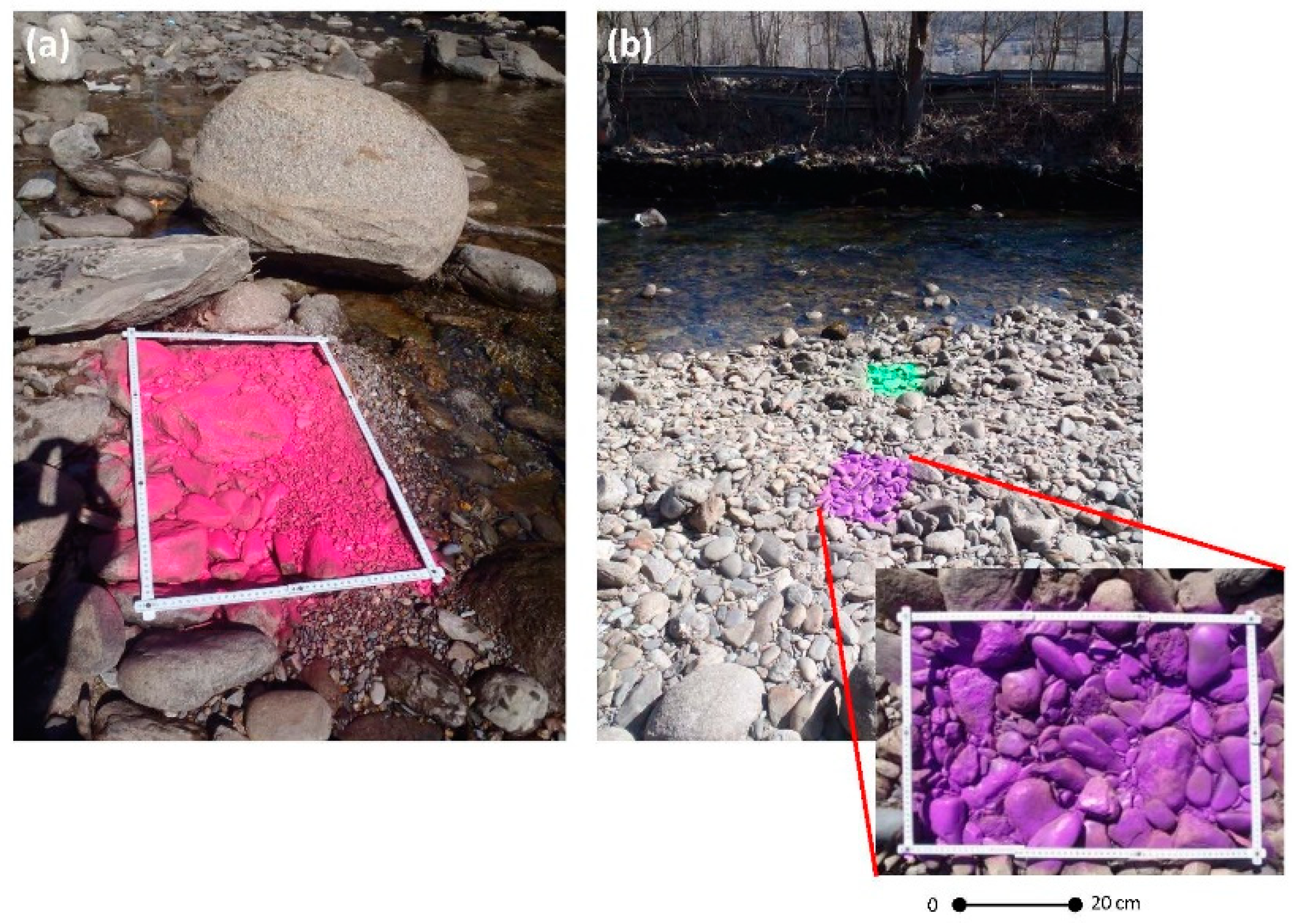
Figure 3.
Surface sediments configurations: (a) Structural bed-material, (b) Coarse surface layer formed by movable cobbles and gravels and (c) Patches of fine sediments (fine gravels and sand).
Figure 3.
Surface sediments configurations: (a) Structural bed-material, (b) Coarse surface layer formed by movable cobbles and gravels and (c) Patches of fine sediments (fine gravels and sand).

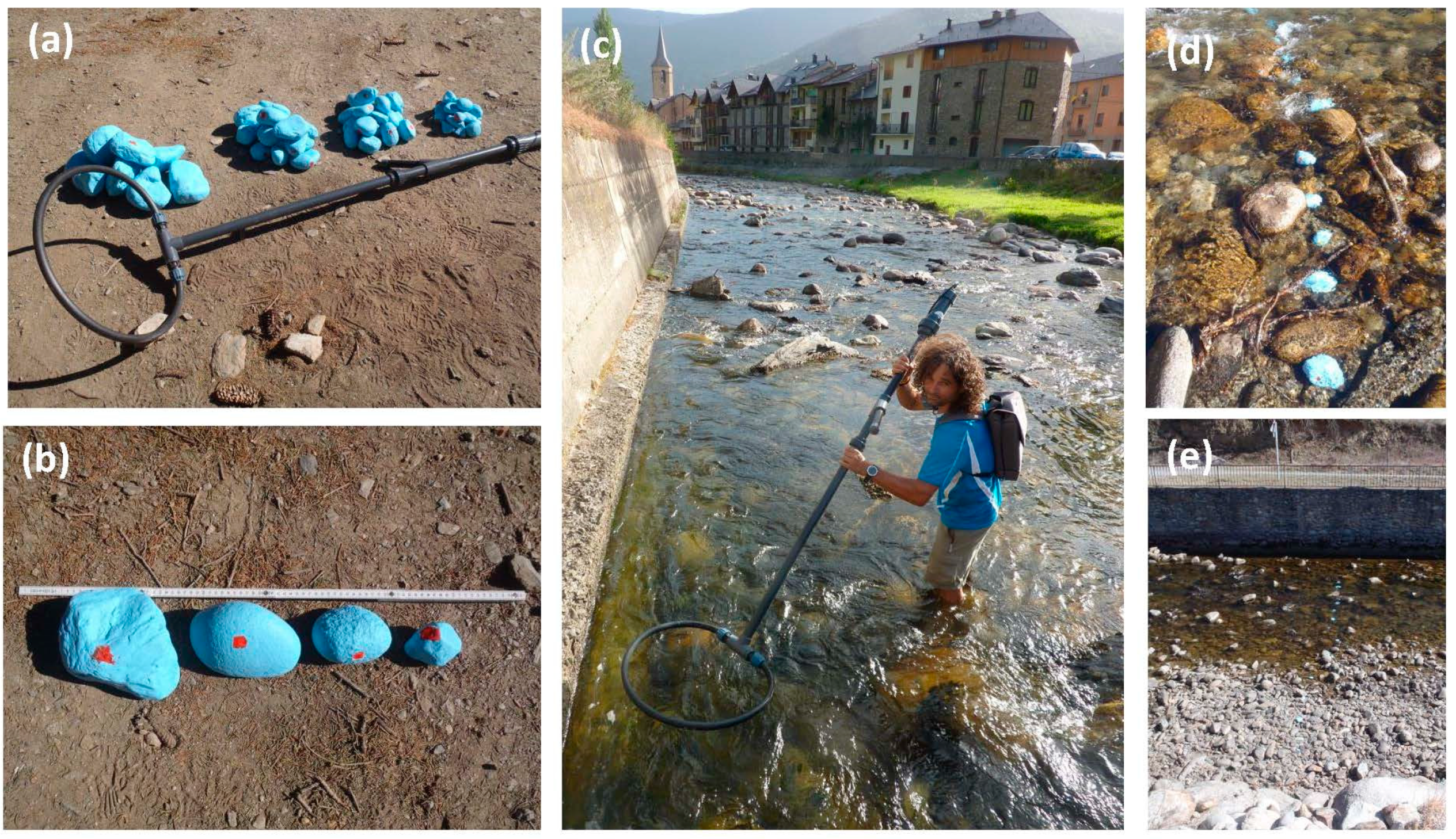
Figure 4.
Painted tracers to monitor bed-material mobility. Examples are for river reaches (a) R2 and (b) R3.
Figure 4.
Painted tracers to monitor bed-material mobility. Examples are for river reaches (a) R2 and (b) R3.

Figure 5.
Examples of RFID tracers deployed in the study reaches. This technique was used in reaches R1 (reference) and R2 (immediately downstream the hydropower station). (a,b) Tracers and equipment used. (c) Recovering tracers after mobility. (d,e) Tracers seeded in the river-bed of sections R2 and R1 respectively.

Figure 6.
Representative cross-sections for the four study reaches: (a) Reach 1 (R1), (b) Reach 2 (R2), (c) Reach 3 (R3) and (d) Reach 4 (R4).
Figure 6.
Representative cross-sections for the four study reaches: (a) Reach 1 (R1), (b) Reach 2 (R2), (c) Reach 3 (R3) and (d) Reach 4 (R4).

Figure 7.
Grain-size distribution of the study reaches in the Noguera Pallaresa: (a) Coarse Surface Layer and Subsurface materials, and (b) Patches of Fine Sediments. Note that the range of sizes for the structural bed-material configuration is also identified in both distributions as reference.
Figure 7.
Grain-size distribution of the study reaches in the Noguera Pallaresa: (a) Coarse Surface Layer and Subsurface materials, and (b) Patches of Fine Sediments. Note that the range of sizes for the structural bed-material configuration is also identified in both distributions as reference.

Figure 8.
Flow scenarios taken to characterise river’s regime in the Noguera Pallaresa: (a) Small magnitude flood and hydropeaking (Scenario 1); (b) High magnitude flood and hydropeaking (Scenario 2); and (c) A single Hydropeak (Scenario 3).
Figure 8.
Flow scenarios taken to characterise river’s regime in the Noguera Pallaresa: (a) Small magnitude flood and hydropeaking (Scenario 1); (b) High magnitude flood and hydropeaking (Scenario 2); and (c) A single Hydropeak (Scenario 3).

Figure 9.
Flow duration curves for the different hydrological conditions observed in the study reaches.
Figure 9.
Flow duration curves for the different hydrological conditions observed in the study reaches.

Figure 10.
Mobility of tracer stones in the study reaches: step-length and GSD of mobilised particles: (a,b) Scenario 1 (Small magnitude flood plus hydropeaking); (c,d) Scenario 2 (High magnitude flood and hydropeaking); and (e,f) Scenario 3 (Single hydropeak, see Section 3.2 for details).
Figure 10.
Mobility of tracer stones in the study reaches: step-length and GSD of mobilised particles: (a,b) Scenario 1 (Small magnitude flood plus hydropeaking); (c,d) Scenario 2 (High magnitude flood and hydropeaking); and (e,f) Scenario 3 (Single hydropeak, see Section 3.2 for details).

Figure 11.
Relation linking (a) critical shear stress and (b) specific stream power to the mean particle size mobilised. Note that the critical shear stress and the specific stream power values are attributed to the peak flows of each hydrological scenario (see Section 4.2 for details). Note that a lineal model is fitted to all data together with the R2 of the relationship. Even so, these models aim at indicating the general trend but in any case the objective is to predict bed mobility.

Figure 12.
Fine sediment availability in reach R3, downstream from the confluence of the River Unarre (see Figure 1 for locations details). (a) General view of the coarse surface layer with a marginal presence of fine after a series of hydropeaks (depletion). The red square illustrates the location of the photo presented in (b) where fine sediments transferred and deposited after a flood event can be clearly observed.

Figure 13.
Conceptual diagram showing the two general bed mobility models in hydropeaked rivers according to their frequency of occurrence.
Figure 13.
Conceptual diagram showing the two general bed mobility models in hydropeaked rivers according to their frequency of occurrence.

Figure 14.
Conceptual model of spatial and temporal river-bed dynamics in hydropeaked reaches based on the observed bed mobility patterns (Figure 12).
Figure 14.
Conceptual model of spatial and temporal river-bed dynamics in hydropeaked reaches based on the observed bed mobility patterns (Figure 12).


Table 1.
Characteristic grain-size values of the various sedimentary fractions of the river-bed (see Section 3.3 for methodological details).
Table 1.
Characteristic grain-size values of the various sedimentary fractions of the river-bed (see Section 3.3 for methodological details).
| Characteristic Grain-Size Values | Surface Sediments Configurations | Subsurface Sediments | ||||||||||||||
|---|---|---|---|---|---|---|---|---|---|---|---|---|---|---|---|---|
| Structural Bed-Material | Coarse Surface Layer (Movable) | Patches of Fine Sediments | ||||||||||||||
| R1 | R2 | R3 | R4 | R1 | R2 | R3 | R4 | R1 | R2 | R3 | R4 | R1 | R2 | R3 | R4 | |
| Proportion (%) | 15 | 10 | 5 | 4 | 67 | 78 | 77 | 74 | 18 | 12 | 18 | 22 | - | - | - | - |
| Percentile 16 (D16) | - | - | - | - | 29 | 32 | 35 | 34 | 0.66 | 0.60 | 0.58 | 0.56 | 1.4 | - | 2.3 | - |
| Percentile 50 (D50) | 881 | 717 | 442 | 373 | 52 | 64 | 63 | 65 | 1.12 | 0.88 | 0.82 | 0.73 | 9.7 | - | 18 | - |
| Percentile 84 (D84) | - | - | - | - | 126 | 136 | 120 | 117 | 2.37 | 1.53 | 1.40 | 1.21 | 58 | - | 62 | - |
| Sorting (σF&W) | - | - | - | - | 1.18 | 1.05 | 0.98 | 0.98 | 0.89 | 0.68 | 0.65 | 0.55 | 2.5 | - | 2.3 | - |
| Armouring (Ar) | - | - | - | - | 5.4 | 3.5 | 3.5 | 3.6 | - | - | - | - | - | - | - | - |
Table 2.
Field observations for the different hydrological scenarios: flow, particles mobilized and step lengths. Note that (i) mobility was measured just in R1 and R2 during scenario 2 (representative of the non-impacted and impacted reaches respectively), and that (ii) no mobility was observed in R4 during scenario 3.
| Reach | Scenario 1 Small Magnitude Flood and Hydropeaking | Scenario 2 High Magnitude Flood and Hydropeaking | Scenario 3 A Single Hydropeak | ||||||||||||
|---|---|---|---|---|---|---|---|---|---|---|---|---|---|---|---|
| Flow (m3/s) | Particle Size Mobilised Coarse Surface Layer (mm) | Step Length (m) | Flow (m3/s) | Particle Size Mobilised Coarse Surface Layer (mm) | Step Length (m) | Flow (m3/s) | Particle Size Mobilised Coarse Surface Layer (mm) | Step Length (m) | |||||||
| Largest | Mean | Longest | Mean | Largest | Mean | Longest | Mean | Largest | Mean | Longest | Mean | ||||
| R1 | 5 | 31 | 1 | - | - | 50 | 171 | 98 | 96 | 29 | - | - | - | - | - |
| R2 | 18 | 41 | 13 | 6.0 | 3.0 | 70 | 146 | 101 | 146 | 42 | 7 | 7 | 5 | 1.5 | 1.4 |
| R3 | 18 | 42 | 21 | 1.8 | 0.9 | 70 | - | - | - | - | 7 | 62 | 17 | 7.1 | 2.6 |
| R4 | 18 | 38 | 13 | 2.3 | 0.9 | 70 | - | - | - | - | 7 | - | - | - | - |
Table 3.
Hydraulic estimations associated to largest particle mobilized for the different hydrological scenarios. Note that (i) mobility was measured just in R1 and R2 during scenario 2 (representative of the non-impacted and impacted reaches respectively), and that (ii) no mobility was observed in R4 during scenario 3.
| Reach | Entrainment Thresholds | ||||||||
|---|---|---|---|---|---|---|---|---|---|
| Observed Values | |||||||||
| Scenario 1 | Scenario 2 | Scenario 3 | |||||||
| Largest Particle (mm) | Shear Stress (N/m2) | Specific Stream Power (W/m2) | Largest Particle (mm) | Shear Stress (N/m2) | Specific Stream Power (W/m2) | Largest Particle (mm) | Shear Stress (N/m2) | Specific Stream Power (W/m2) | |
| R1 | 31 | 48 | 46 | 171 | 124 | 303 | - | - | - |
| R2 | 41 | 36 | 88 | 174 | 99 | 305 | 7 | 29 | 37 |
| R3 | 42 | 42 | 73 | - | - | - | 62 | 32 | 37 |
| R4 | 38 | 33 | 67 | - | - | - | - | - | - |
Table 4.
Entrainment thresholds in the study reaches of the Noguera Pallaresa: Predicted shear stress values for representative percentiles of the coarse surface layer and for the largest particles mobilised.
Table 4.
Entrainment thresholds in the study reaches of the Noguera Pallaresa: Predicted shear stress values for representative percentiles of the coarse surface layer and for the largest particles mobilised.
| Reach | Entrainment Thresholds | |||||||||
|---|---|---|---|---|---|---|---|---|---|---|
| Predicted Values of Critical Shear Stress | ||||||||||
| Percentile 16 (D16) | Percentile 50 (D50) | Percentile 84 (D84) | Largest Particle Mobilised (Predicted vs. Observed) | |||||||
| Size (mm) | Shear Stress (N/m2) | Size (mm) | Shear Stress (N/m2) | Size (mm) | Shear Stress (N/m2) | Size (mm) | Predicted Shear Stress (N/m2) | Observed Shear Stress (N/m2) | Residual (Observed—Predicted) | |
| R1 | 29 | 21 | 52 | 38 | 126 | 91 | 171 | 124 | 124 | 0 |
| R2 | 32 | 23 | 64 | 47 | 136 | 99 | 174 | 127 | 99 | −28 |
| R3 | 35 | 25 | 63 | 46 | 120 | 87 | 62 | 45 | 32 | −13 |
| R4 | 34 | 25 | 65 | 47 | 117 | 86 | 38 | 28 | 33 | 5 |
© 2020 by the authors. Licensee MDPI, Basel, Switzerland. This article is an open access article distributed under the terms and conditions of the Creative Commons Attribution (CC BY) license (http://creativecommons.org/licenses/by/4.0/).
Share and Cite
MDPI and ACS Style
Vericat, D.; Ville, F.; Palau-Ibars, A.; Batalla, R.J. Effects of Hydropeaking on Bed Mobility: Evidence from a Pyrenean River. Water 2020, 12, 178. https://doi.org/10.3390/w12010178
AMA Style
Vericat D, Ville F, Palau-Ibars A, Batalla RJ. Effects of Hydropeaking on Bed Mobility: Evidence from a Pyrenean River. Water. 2020; 12(1):178. https://doi.org/10.3390/w12010178
Chicago/Turabian StyleVericat, Damià, Fanny Ville, Antonio Palau-Ibars, and Ramon J. Batalla. 2020. "Effects of Hydropeaking on Bed Mobility: Evidence from a Pyrenean River" Water 12, no. 1: 178. https://doi.org/10.3390/w12010178
Note that from the first issue of 2016, this journal uses article numbers instead of page numbers. See further details here.