Numerical Studies on the Suitable Position of Artificial Upwelling in a Semi-Enclosed Bay

Abstract

Ecological engineering by artificial upwelling is considered a promising way to improve water quality. Artificial upwelling could lift nutrient-rich bottom water to the surface, enhance seaweed growth and consequently increase nutrient removal from seawater. However, one of the major obstacles of the engineering application is to determine the suitable position of ecological engineering, which is critical for artificial upwelling’s performance. In this paper, potential artificial upwelling positions in a semi-closed bay are simulated by using the unstructured-grid Finite-Volume Coastal Ocean Model (FVCOM). The results show that the upwelling position with relative small tidal current and close to corner will be helpful to increasing nutrient concentration of surface water, and be appropriate to build the ecological engineering. With proper design of the ecological engineering, it is possible to have a noticeable impact in semi-closed bay. Thus, artificial upwelling has the potential to succeed as a promising way to alleviate the eutrophication.

1. Introduction

In recent years, with the development of industry and agriculture as well as a highly growing population in coastal areas, the deterioration of water quality become a global problem [1,2,3]. Using seaweed farming to remove excess nutrients is proposed and considered as an environmentally friendly and economical way [4,5].

Seaweed can take up dissolved nutrients, and then by harvesting the seaweed, nutrients are removed to land [6]. Nutrient removal capability of large-scale Chinese seaweed is significant, because the seaweed aquaculture in China is 2/3 of global production. And it is reported that nitrogen (N) and phosphorus (P) concentration are respectively 3.71 ± 1.15 N % DW (dry weight) and 0.52 ± 0.23 P % DW for Saccharina japonica, 4.53 ± 0.43 % DW and 0.34 ± 0.05 P % DW for Gracilariopsis spp., which are the dominant species for Chinese aquaculture. And mean N and P removal of Chinese seaweed farming are respectively 60.31 and 7.60 t km⁻² year⁻¹ [7]. However, high-density seaweed aquaculture can slow down the water circulation and the renewal of surface water, which lead to regional and temporary nutrient deficiency [8,9,10,11]. To relieve nutrient limitations and promote the production of seaweed, artificial upwelling attracts scientific and policy interest.

On the one hand, artificial upwelling can lift nutrient-rich bottom water to euphotic layer [12,13], and be used to stimulate the growth of phytoplankton, seaweed and algae [14]. On the other hand, by mixing surface and bottom water, artificial upwelling can destroy density stratifications to alleviate 3 the shortage of oxygen and strengthens the vertical exchange of water [15]. Furthermore, it is found that the implementation of artificial upwelling system has a good effect on adjusting the ratio of nitrogen to phosphorus in seawater [16] and increasing chlorophyll-a concentration [17,18]. There have been some artificial upwelling systems which are verified to have some ecological effects, for example, “wave pump” is used to change the ratio of nitrogen to phosphorus in Hawaii [16], “perpetual salt fountain” is proved to increase primary production in the ocean [19], “air-bubble curtains” in Norway can enhance the environmental conditions for the growth of non-toxic algae [18], ‘TAKUMI’ and density current generator has been used to enhancing water quality in Japan [18,20].

In this research, Aoshan Bay is used as the typical semi-closed bay for the field application of artificial upwelling (shown in Figure 1).

The length of the bay mouth and the area of the whole bay are 15 km and 164 km², respectively. The maximum and mean water depth are respectively 13 m and 5 m. The change of mean temperature is obviously, the highest and lowest mean temperature are respectively 28 °C in August and 4 °C in March. The change of salinity is not significant, the highest and lowest mean salinity are respectively 32.0 and 31.4 [21]. This bay has been used for seaweed agriculture, but the agriculture is suspended temporarily for nutrient deficiency, which leads to the algae declining in high-density seaweed aquaculture. The air-injection system is powered by solar platform and used to bring nutrient-rich water up to the aquaculture area of seaweed (Figure 2). The detailed description of the system can be found in our previous study [22]. However, one of the key factors for artificial upwelling success is to find the appropriate position to place artificial upwelling. Without the suitable position, artificial upwelling maybe inefficiency or even useless. This paper is aimed to find the appropriate artificial upwelling positions in a semi-closed bay and discuss the effect of running time (days after start of artificial upwelling) and spring-neap tide to the spreading and accumulation of artificial upwelling. An unstructured grid finite-volume coastal ocean model (FVCOM) was used to understand the effect of the artificial upwelling. This model was developed originally by Chen et al. [23] and efficient in resolving complex estuaries and coastal oceans dynamics. The unstructured triangular grid system can successfully embody the islands and barriers with complex topographies. The wet/dry treatment technique is a method, which is used to simulate the water draining out and flooding onto of the inter-tidal zone. In this way, FVCOM is suitable for evaluating the spreading of nutrient-rich bottom water.

2. Methods

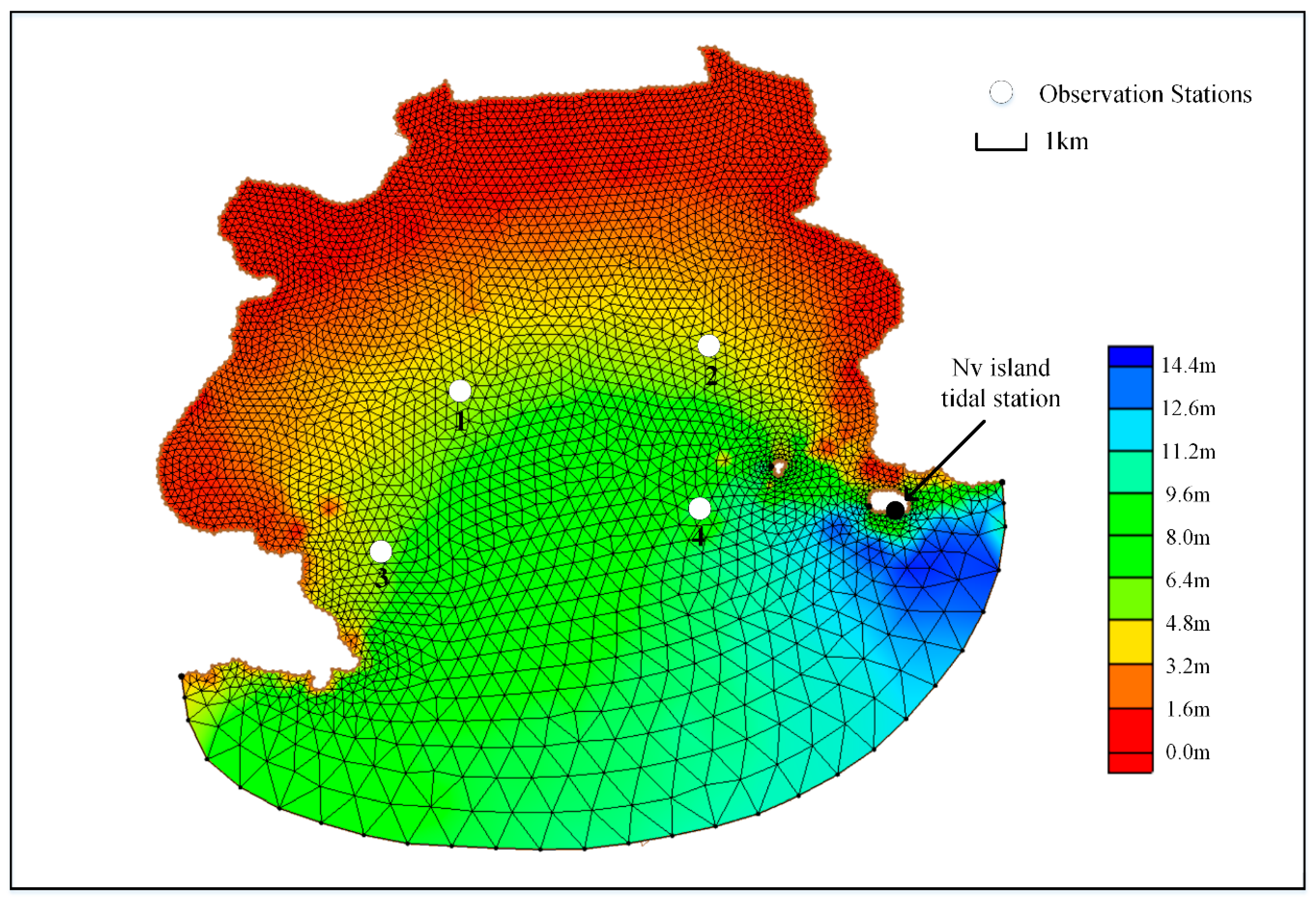
2.1. Design of Numerical Experiments

The unstructured-grid Finite-Volume Coastal Ocean Model (FVCOM) was used to conduct the numerical experiments in a semi-closed bay. FVCOM uses a modified Mellor and Yamada level 2.5 (MY-2.5) turbulence closure schemes [24] for vertical eddy mixing and Smagorinsky turbulent closure schemes [25] for the horizontal eddy viscosity and diffusivity. Unstructured triangular meshes have advantages in fitting irregular coastal boundary. Irregular bottom topography is represented by using $\sigma$ transformation, which can improve numerical efficiency and provide good numerical results. More details information about FVCOM can be found in Chen’s paper et al. [26].

The $\sigma$ coordinate system is used to represent the bottom topography. The $\sigma$ coordinate transformation is shown as $\sigma =\frac{z-\zeta }{H+\zeta }=\frac{z-\zeta }{D}$, where $H$ is reference depth to mean surface level, $\zeta$ is height of free surface, $D$ is total water column depth.

The advection–diffusion equations of temperature and salinity are coupled to the governing equations:

$$\frac{\partial TD}{\partial t}+\frac{\partial TuD}{\partial x}+\frac{\partial TvD}{\partial y}+\frac{\partial Tw}{\partial \sigma }=\frac{1}{D}\frac{\partial }{\partial \sigma }\left(K_h\frac{\partial T}{\partial \sigma }\right)+D{F}_T$$

(1)

$$\frac{\partial SD}{\partial t}+\frac{\partial SuD}{\partial x}+\frac{\partial SvD}{\partial y}+\frac{\partial Sw}{\partial \sigma }=\frac{1}{D}\frac{\partial }{\partial \sigma }\left(K_h\frac{\partial S}{\partial \sigma }\right)+D{F}_S$$

(2)

$$D{F}_T\approx \left[\frac{\partial }{\partial x}\left(A_{h}H\frac{\partial T}{\partial x}\right)+\frac{\partial }{\partial y}\left(A_{h}H\frac{\partial T}{\partial y}\right)\right]$$

(3)

$$D{F}_S\approx \left[\frac{\partial }{\partial x}\left(A_{h}H\frac{\partial S}{\partial x}\right)+\frac{\partial }{\partial y}\left(A_{h}H\frac{\partial S}{\partial y}\right)\right]$$

(4)

where T is the temperature; S is the salinity; $F_T$ and $F_s$ represent thermal and salt diffusion terms;

The change of sea temperature, caused by net downward shortwave radiation, net downward longwave radiation, sensible fluxes and latent fluxes, has little influence on artificial upwelling simulation. And it is not our key point of this research. Hence, the surface net heat flux is not concluded in this simulation. The boundary condition on the sea surface ($\sigma =0$) and sea bottom ($\sigma =-1$):

$$\frac{\partial T}{\partial \sigma }=0$$

(5)

A wet/dry point treatment method [27] is used in this simulation, which includes a viscous sublayer to stable the model at the intertidal zone. The wet or dry criterion for the node points is given as:

$$\{\begin{array}{l}\mathrm{wet},\mathrm{if}D=H+\zeta >D_{\min }\hfill \\ \mathrm{dry},\mathrm{if}D=H+\zeta \le D_{\min }\hfill \end{array}$$

(6)

In this simulation, $D_{\min }$ was 10.0 cm for stability of the model.

As shown in Figure 3. The grid size is divided into three parts, open boundary grid size is approximately 1000 m to increase simulation efficiency, the grid of coastal area is 180 m to evaluate the tidal flat’s effect, the grid size of island is about 100 m to evaluate the influence of these island. The vertical resolution is about 1.5 m at open boundary and less than 0.3 m at intertidal zone by using tenth sigma levels. There are 8091 triangular elements and 4233 nodes in this model domain. The time step of the external and internal modes are 1 s and 10 s respectively. The detailed information about the key parameters for the artificial upwelling system is shown in

Table 1. Key Parameters for the artificial upwelling system of Aoshan Bay.

Model Parameter	Value
External Timestep (s)	1
Internal time split (s)	10
Horizontal diffusion	Smagorinsky scheme
Vertical eddy viscosity	M-Y 2.5 turbulent closure
Open boundary condition	TPXO
Nodes, elements, vertical layers	4233, 8091, 10 uniform $\sigma$ layer
Smagorinsky constant	0.2
Horizontal Prandtl number	1
Vertical Prandtl number	1
Vertical mixing coefficient	10−6
Minimum Bottom Roughness (m)	0.0025
Roughness length (m)	0.001

.

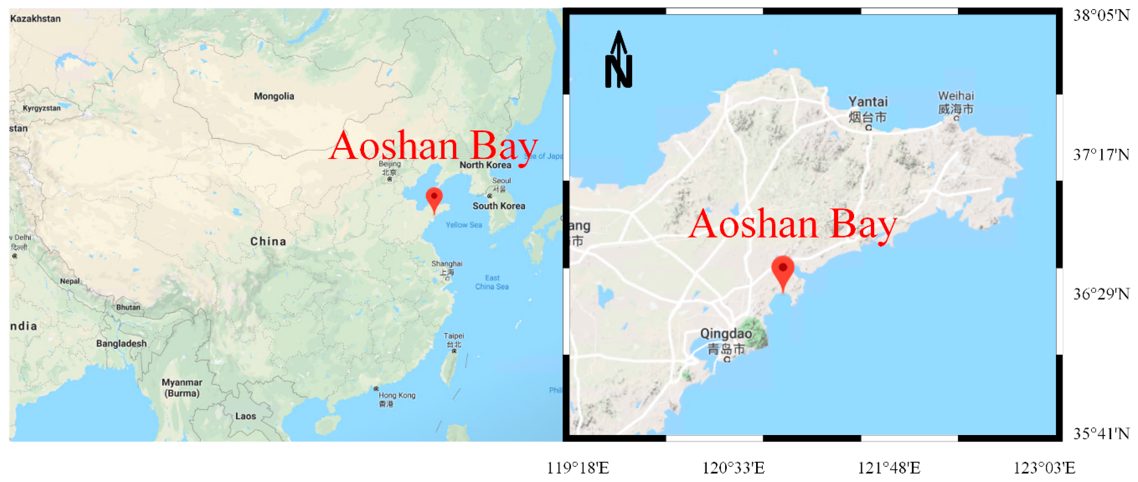
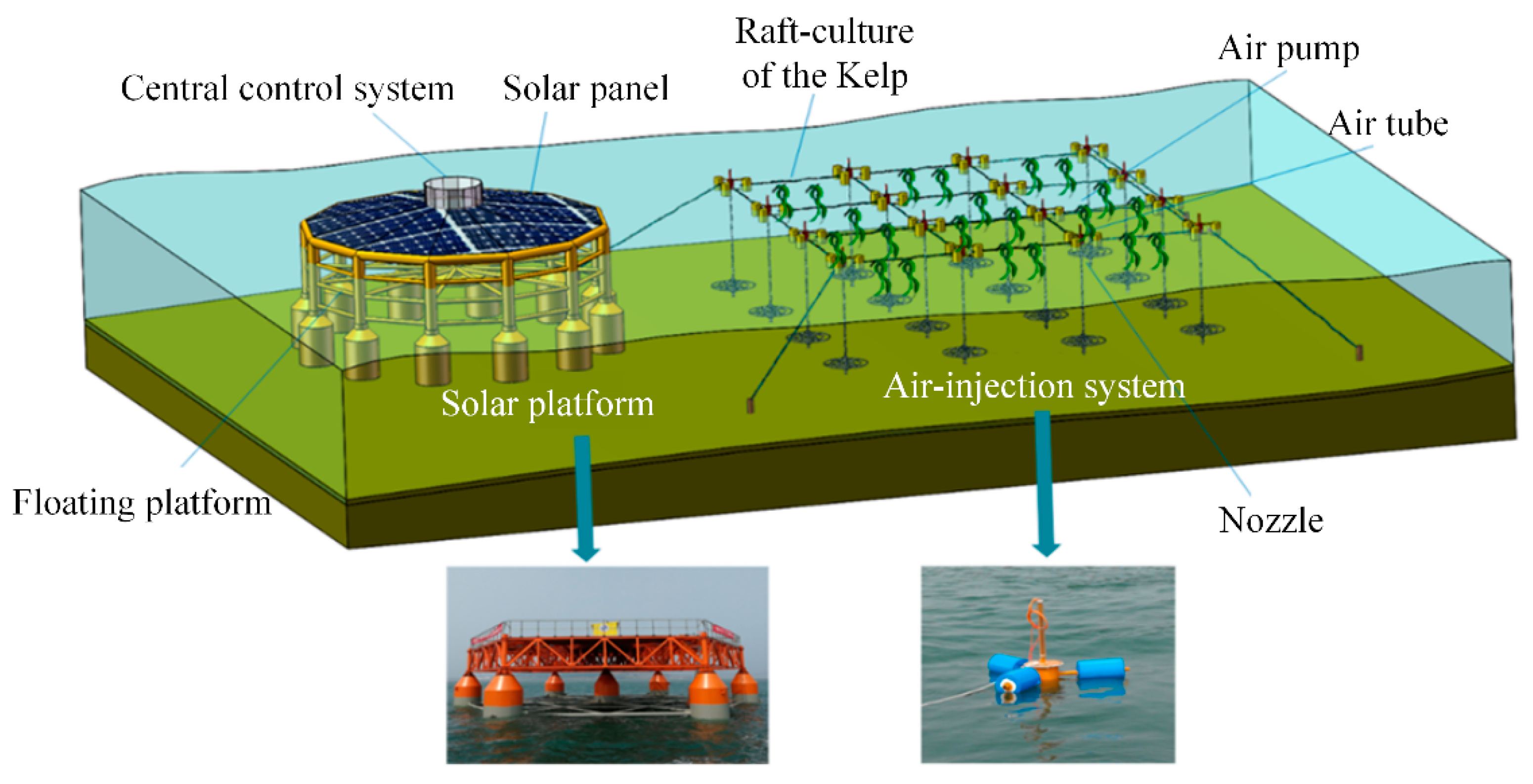
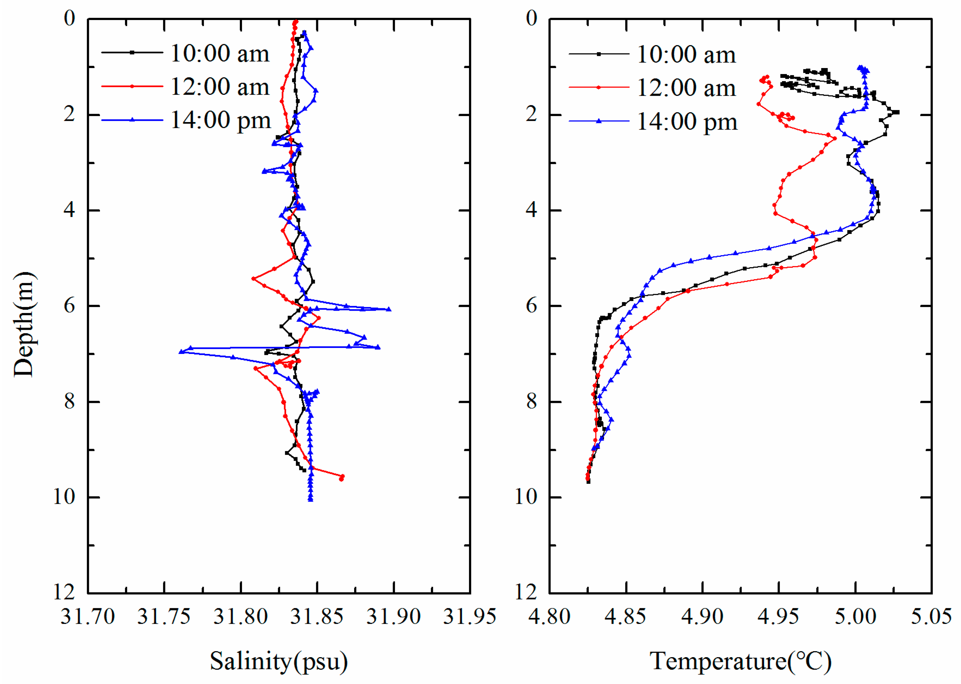
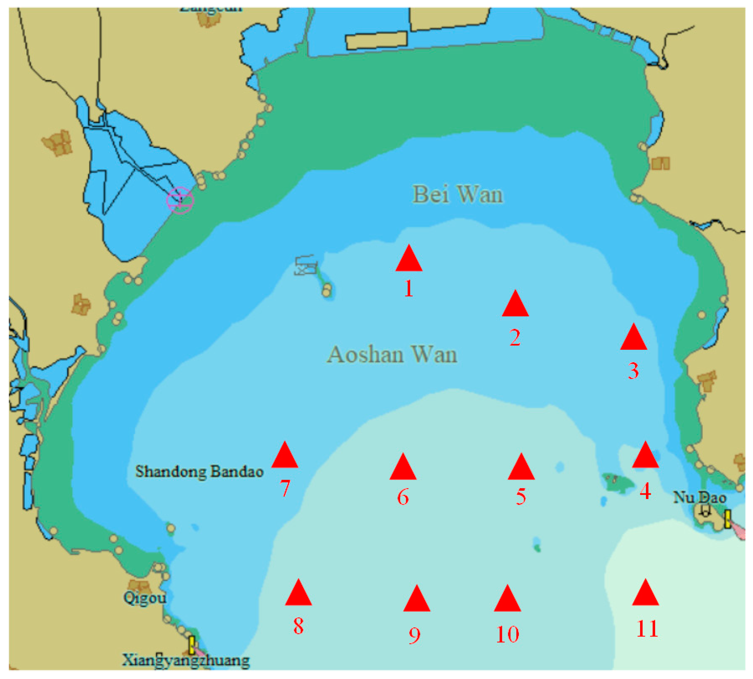
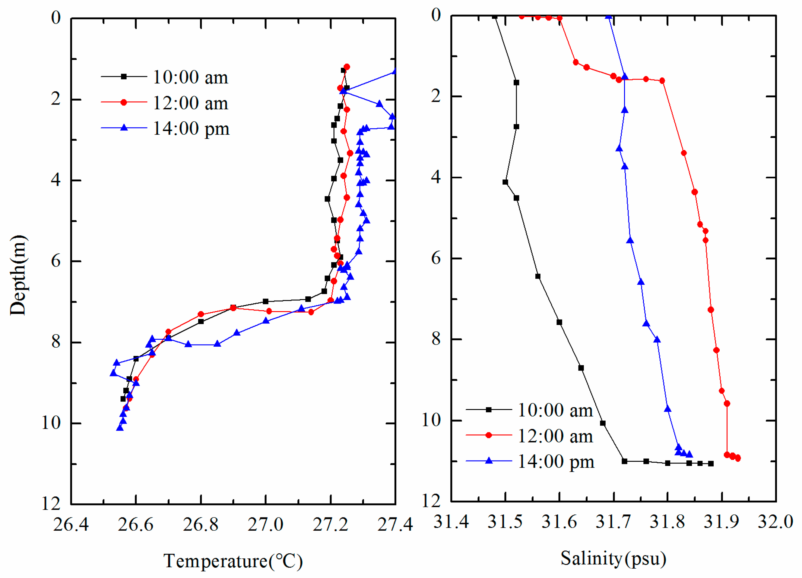
2.2. Field Measurements

The initial temperature and salinity values in Aoshan Bay were obtained from the mean value of field measurement in 18 January 2019 (Figure 4). The difference of salinity between sea surface and bottom is very small. But the temperature difference between surface and bottom is relative significant. In this model, initial surface sea surface temperature is 5.0 °C and bottom temperature is 4.8 °C, the boundary condition at south open boundary also has the same temperature distribution. According to the change of temperature, an index (upwelling ratio, Ra) is defined as the percent of the variation of sea surface temperature caused by artificial upwelling. By monitoring the change of sea surface temperature, we can calculate the percent of bottom water advected by upwelling in surface water. For example, if the percent of temperature variation in surface water is 0.2%, Ra is 0.002. Salinity is assumed to be the same in the whole bay to simplify the simulation. Hence, the salinity at open boundary is also a constant (31.8, according to Figure 4).

The system is designed to run from 10:00 a.m. to 12:00 a.m. every day. Hence, in the simulation, the artificial upwelling also starts to run at 10:00 for two hours every day with water discharged equaled to 1.2 m³/s. The information about background value of Aoshan Bay and key parameters of artificial upwelling are shown in

Table 2. Background value of Aoshan Bay and key parameters of artificial upwelling.

Initial sea surface temperature (°C)	5.0
Initial sea bottom temperature (°C)	4.8
Initial salinity value	31.8
Water discharged from artificial upwelling (${\mathrm{m}}^3/\mathrm{s}$)	1.2
Running time of the system ($\mathrm{hour}/\mathrm{day}$)	2 (10:00–12:00 a.m.)

.

3. Results

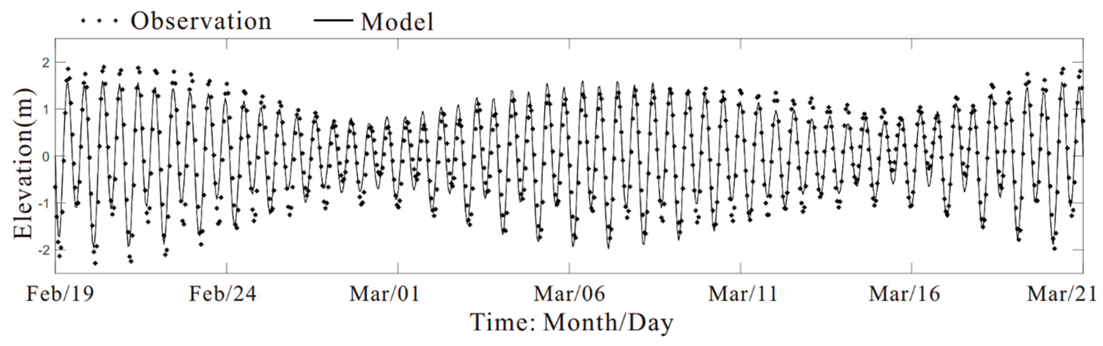
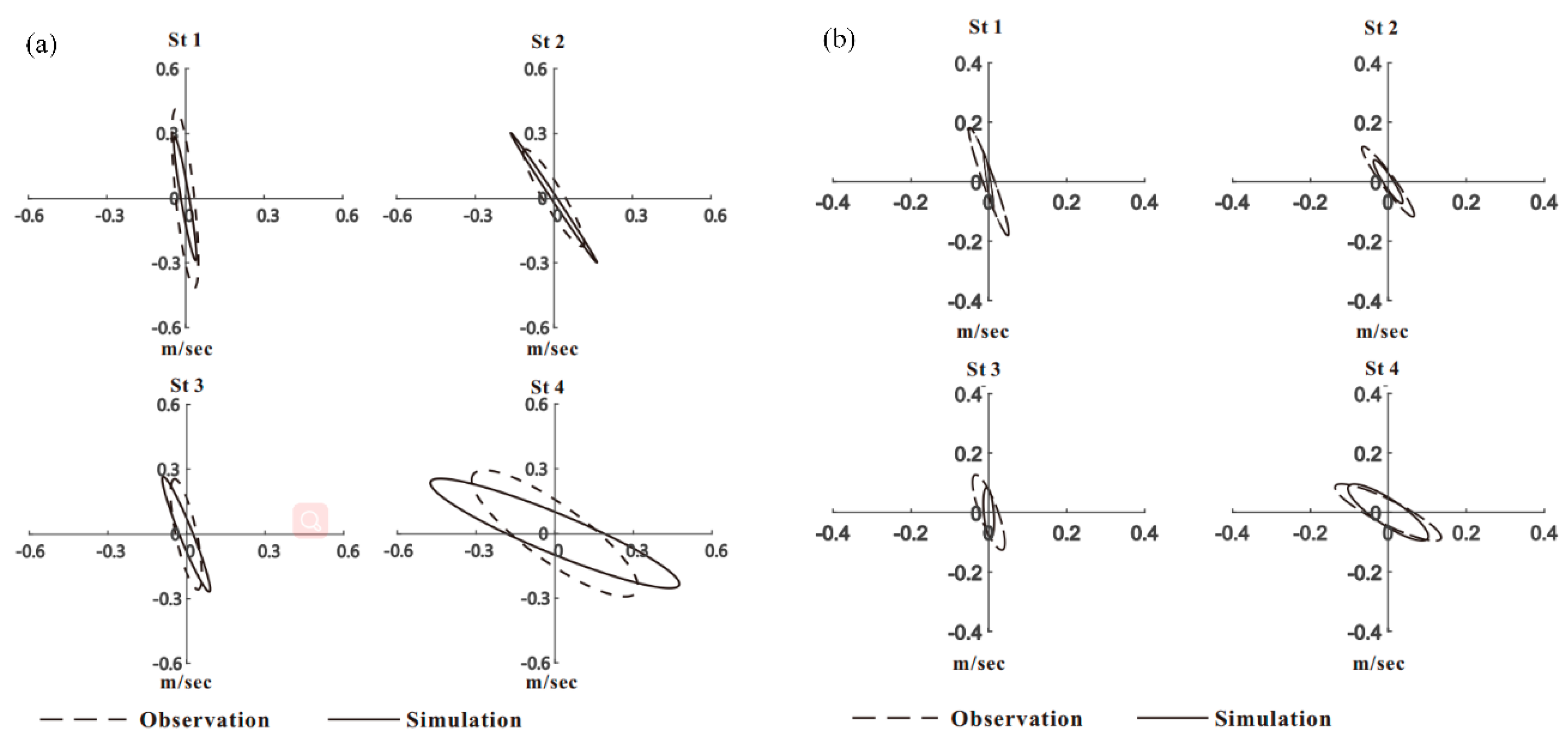
3.1. Model Verification

To verify the numerical model, the surface elevation and tidal current ellipses obtained by field observation are compared with simulation results. First of all, the observed surface elevation is measured at Nv island tidal station (Figure 3) and provided by China National Marine Science Data Sharing Service Platform (http://mds.nmdis.org.cn/). As we can see from Figure 5, the simulation results of tidal elevation basically agreed with the observed results for 30 days, with R-square (the determination coefficient of the correlation between observed and simulated) equals to 0.79. The observed sea area is typical semi-diurnal tides. The results show good fitness during neap tide but some difference during spring tide. The ranges of tidal fluctuation for neap and spring tide are respectively 1.45 and 3.53 m.

Secondly, as shown in Figure 6, two main tidal constituents (M2 and S2) obtained by field observation and simulation results at four stations (marked in Figure 3) are compared. In this comparison, the simulation was iso-density and the artificial upwelling system was not operated. As shown in Figure 6, the major directions of simulated tidal current are slightly rotated anticlockwise compared with the observed, the deviation between observation and simulation results is less than 20°. Although there is some difference between the calculated and measured value, the magnitudes of calculated current results are basically comparable with the measured, the deviation of velocity is less than 0.1 m/s. In conclusion, the model results, with acceptable errors, show basically agreement with the observed results of surface elevation and tidal current. As a result, this model can be used to simulate the water dynamics in Aoshan Bay.

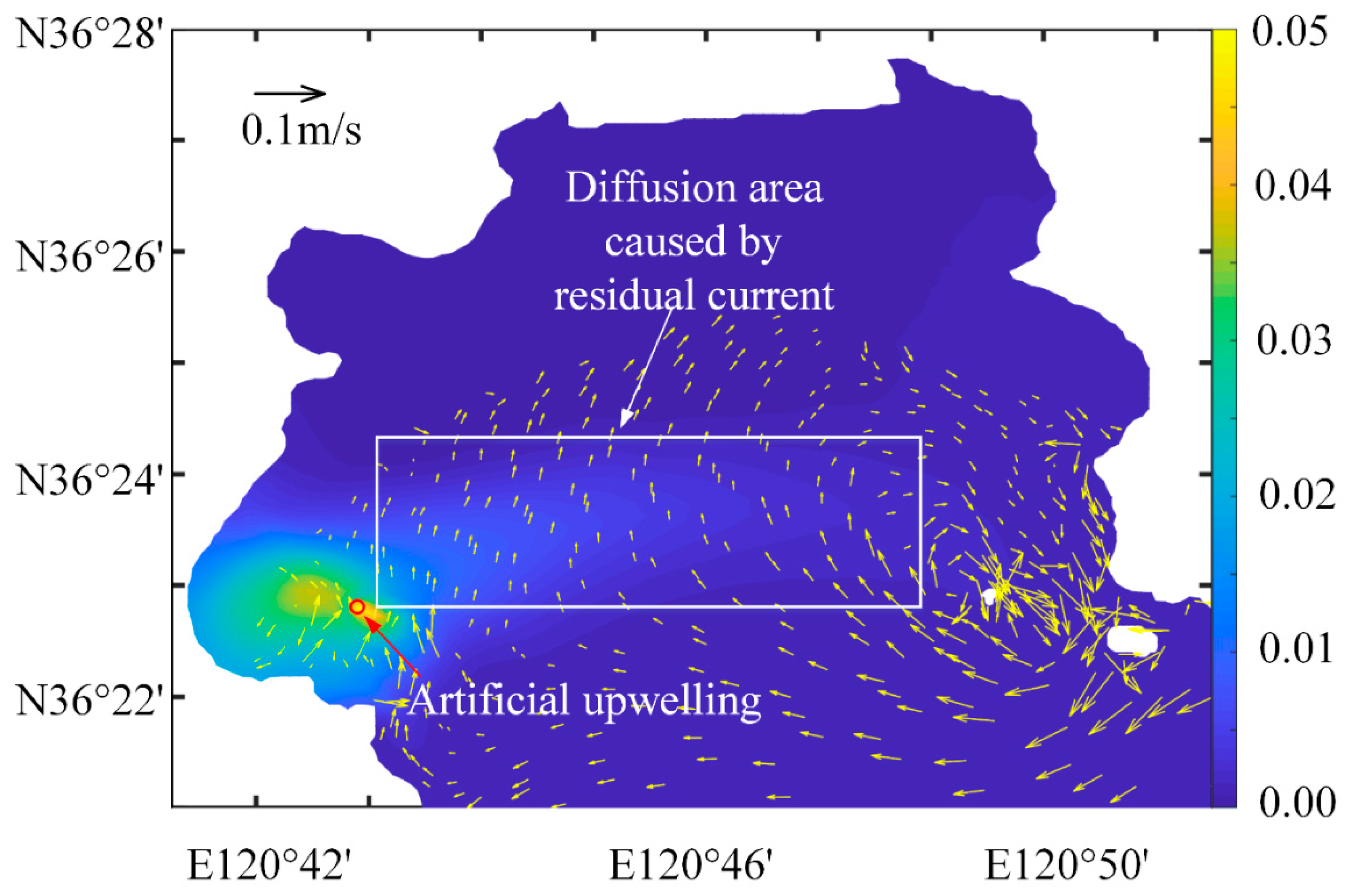
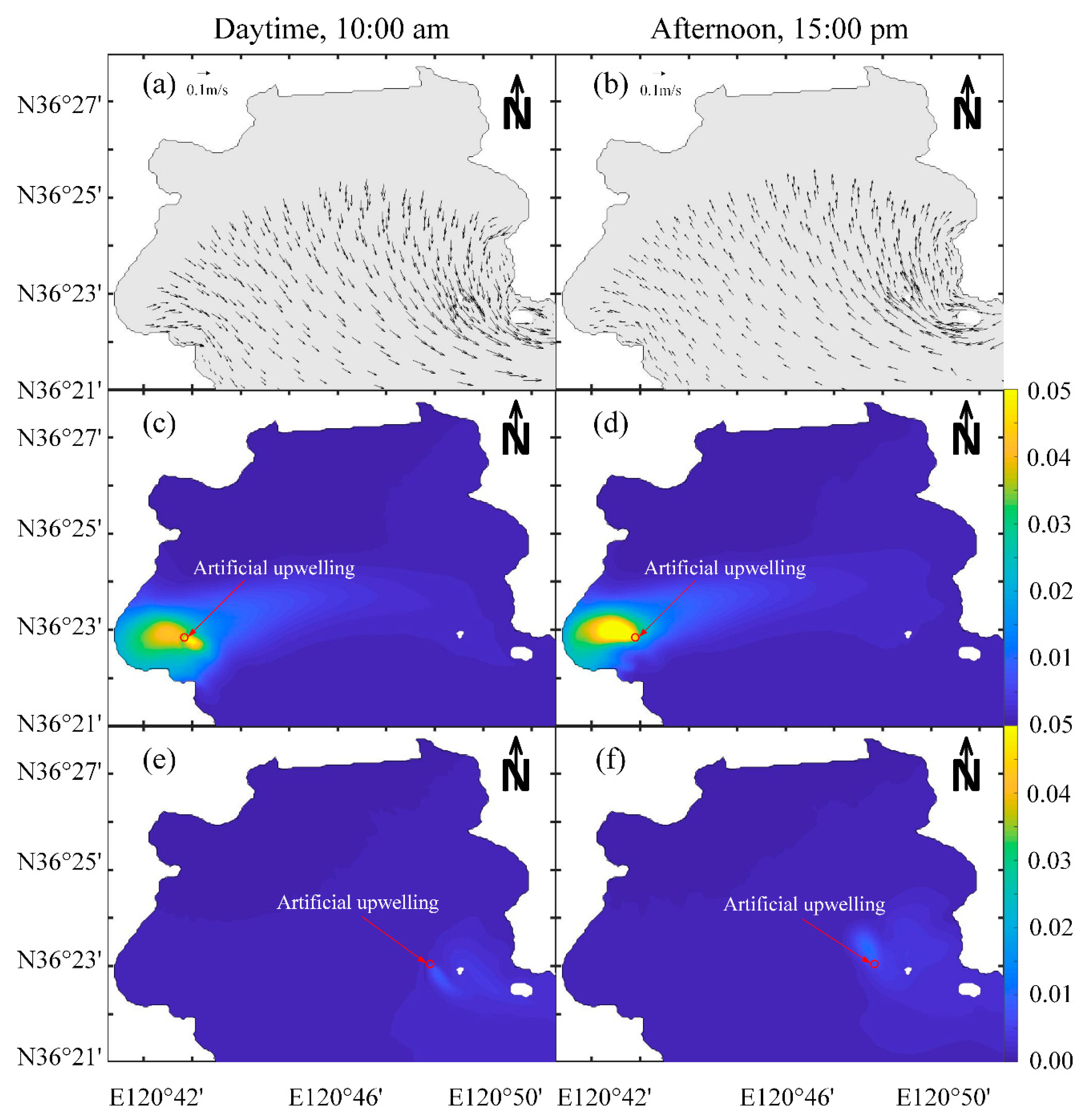
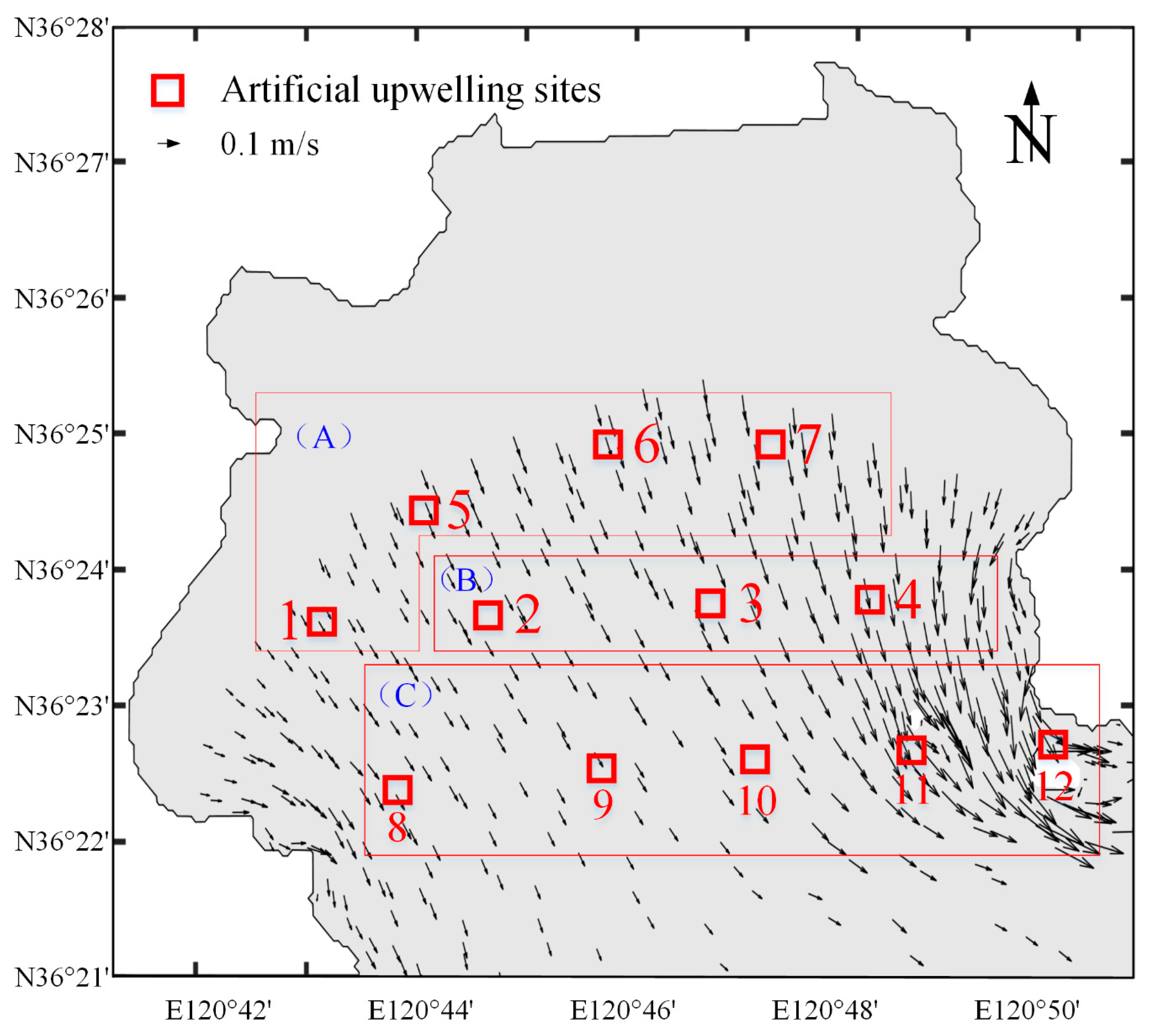
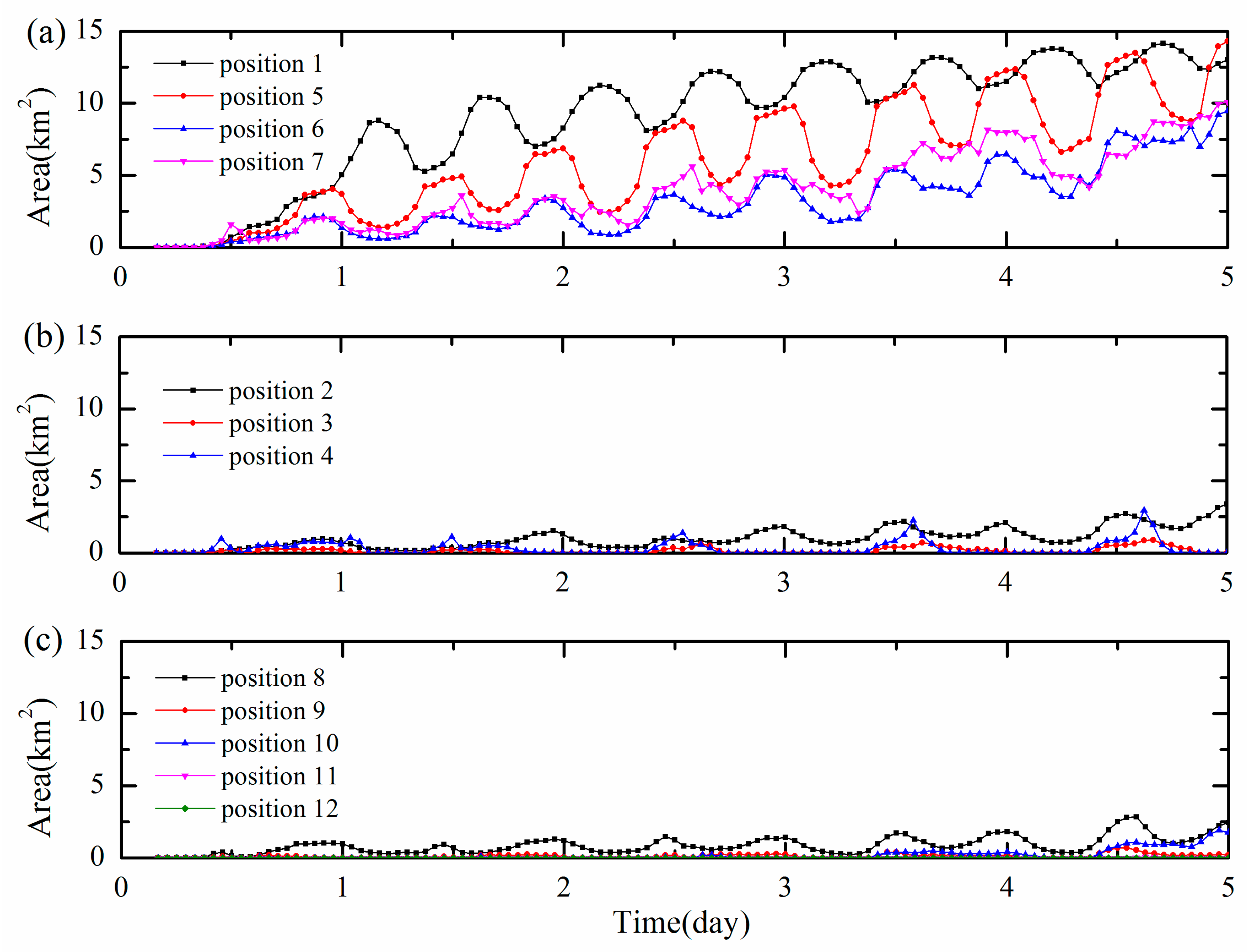
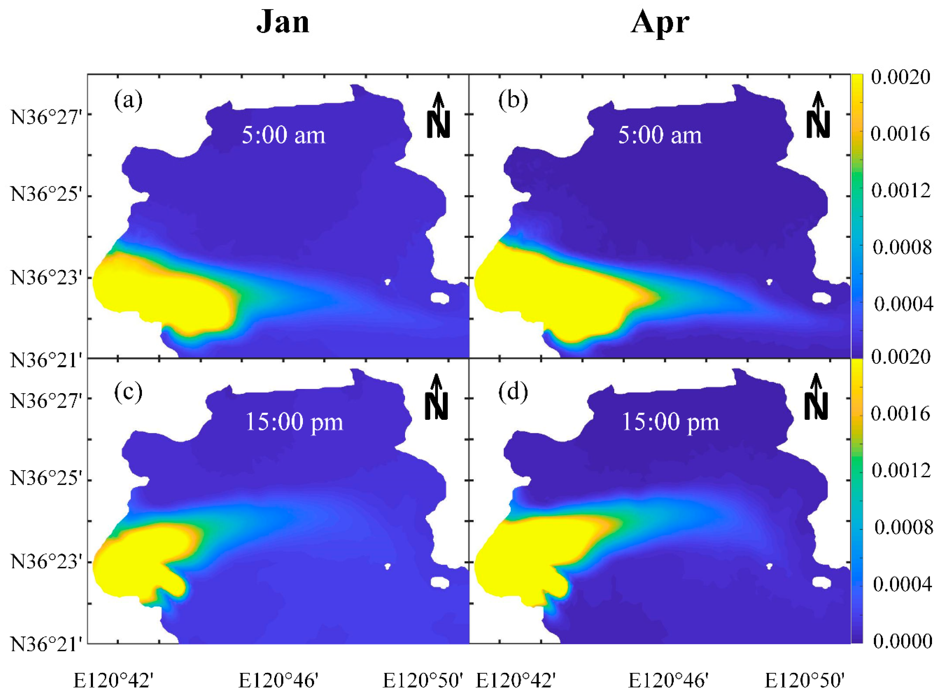
3.2. The Effect of Tidal and Residual Current to Artificial Upwelling

To analyse the diffusion process of upwelling plume in surface water, residual current and tidal current are two major factors. The horizontal distribution of residual current is shown in Figure 7. There are a large residual current circulation and a local circulation at the southwest corner of Aoshan Bay, which are well simulated by numerical simulation. After running artificial upwelling for 10 days in the red circle position, we can see a long tail of artificial upwelling plume, which is marked by the white square in Figure 7. The direction of residual current influence the diffusion direction of upwelling plume, which is northeast. Due to the low velocity of residual current and little volume flow rate of artificial upwelling, the percent of sea surface temperature variation caused by residual current is nearly invisible, which is less than 2% in most part of white square area.

The horizontal distribution of the tidal current is shown in Figure 8. The diffusion conditions are compared in two different positions, which are separately in western and eastern side of Aoshan bay. The distribution of temperature variation is completely different for these two positions. The influence of artificial upwelling in eastern side of bay is more significant (Figure 8c,d), and the magnitude of tidal current velocity plays a critical role. The magnitude of tidal current velocity is relative large in southeastern corner, and gradually decrease along as northwestern direction. Hence, the artificial upwelling position in Figure 8c,d with relative small tidal current velocity is diffused much weaker than the artificial upwelling position in Figure 8e,f.

Compared with residual current, tidal current has bigger velocity and has more significant influence to the diffusion of upwelling plume. However, residual current could transfer the artificial upwelling to the whole bay, which will generate larger influence area.

3.3. The Optimal Artificial Upwelling Positions for Ecological Engineering

According to the effect of tidal and residual current to artificial upwelling, tidal current plays a more important role in the diffusion process of upwelling plume. Hence, based on the tidal current and water depth of Aoshan Bay, 12 possible positions in the semi-closed bay are selected to evaluate the effect of artificial upwelling position (shown in Figure 9). Some areas, in which the water is less than 3 m depth, are not suitable for seaweed farming. Hence, these areas are excluded from potential artificial upwelling positions. Finally, according to the magnitude of tidal current, this semi-closed bay can be divided into three parts (shown in Figure 9): A, this area is relatively far away from the open sea, the tidal current is about 0.1 m/s. B, the area is in the middle of the bay, the tidal current is about 0.2 m/s. C, the area is close to the open sea, the tidal current is about 0.3–0.4 m/s.

Twelve different positions in Aoshan Bay are selected as the potential locations to set up artificial upwelling system (shown in Figure 9). In the simulations, we use the upwelling ratio (R_a) of surface water to evaluate different positions’ influence in semi-closed bay. The variations of area where R_a is bigger than 0.002 in twelve different positions are shown in Figure 10. Twelve positions are divided into three parts A, B and C, according to their distance to open sea, and shown in Figure 9.

For all these positions in Figure 10b,c, the area where R_a are bigger than 0.002 are not larger than 4 km², after running artificial upwelling for 5 days. In Figure 10a, for all positions of part A, the area where R_a is bigger than 0.002 can also reach about 10 km² after running artificial upwelling for 5 days. Hence, compared with part B and C, the positions in part A has significant better performance. By comparing the upwelling positions and the distribution of tidal current in Figure 9, we find that the positions with relative small tidal current velocity has advantage in decreasing the diffusion of upwelling plume.

To learn more about the difference between three parts and configure the accumulation process of upwelling, position 1, 2 and 11 are selected from three parts and horizontal distributions of upwelling ratio in surface water of these positions are shown in Figure 11.

For artificial upwelling position 1, it is rising tide at bay 10:00 am. (Figure 11d). The direction of tide current is benefit to accumulate the upwelling plume. Artificial upwelling system works from 10 to 12 am. And as the increasing of time, the dye concentration gradually increases around position 1. During the ebb tide, the upwelling is still controlled in western corner of bay. Hence, after 5-day running, the dye concentration near position 1 is obviously different from initial situation.

For artificial upwelling position 2, we can find that, after starting artificial upwelling system at 10 am., there is a significant point shown the change of upwelling ratio (Figure 11e). And the upwelling is diluted to open sea by tidal current at 15:00 and 20:00 p.m. (Figure 11h,k). For artificial upwelling position 11, which is closer to open sea and has larger tidal current velocity, the most part of artificial upwelling is transferred to open sea with the ebb tide (Figure 11i,l). Hence, position 11 does not have a good performance in accumulating artificial upwelling plume.

In conclusion, part A has better performance in maintaining the influence of artificial upwelling. Part A has relative small tidal current. And the residual current forms a circulation in the western corner of Aoshan bay, which makes position 1 be beneficial for the accumulation of artificial upwelling. As the decrease of distance to the open sea, the tidal current become larger. And for part B and C, artificial upwelling is more easily to be diluted to open sea. Hence, part B and C are not suitable to set up artificial upwelling. The conclusion is also suitable for other artificial upwelling devices, which is used in the semi-closed bay.

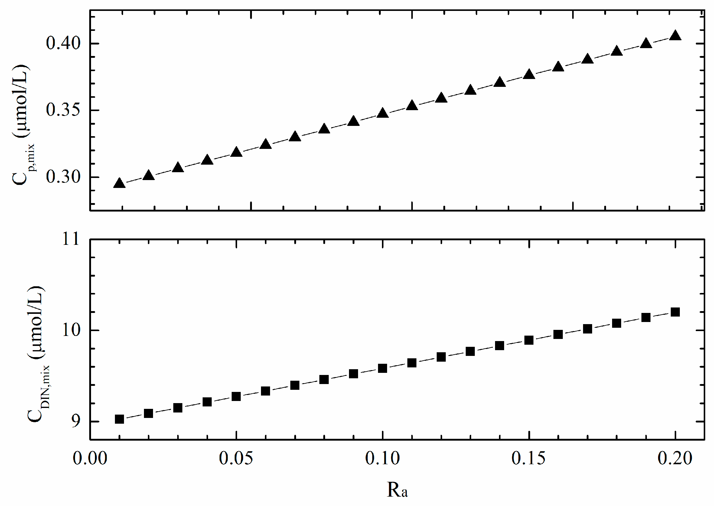
3.4. The Performance of Artificial Upwelling in Increasing Nutrient Concentration

After determining the appropriate position of artificial upwelling, there is still a critical problem for this study: artificial upwelling’s performance in increasing nutrient concentration. To know the specific value of nutrient concentration in surface water after using artificial upwelling, the concentration could be calculated by the following equations:

$$C_{P,mix}=C_{P,sur}\times (1-R_a)+C_{P,ove}\times R_a$$

(7)

$$C_{DIN,mix}=C_{DIN,sur}\times (1-R_a)+C_{DIN,ove}\times R_a$$

(8)

where C is the concentration of nutrients, the subscripts P and DIN are respectively phosphate and dissolved inorganic nitrogen, the subscripts sur and bot means surface water and overlying water, and the subscript mix is the surface water mixed with artificial upwelling. R_a is the percent of the variation of sea surface temperature caused by artificial upwelling.

To show the variation of nutrient concentration more clearly, the nutrient concentration of Aoshan bay could be used as the background value. For Aoshan Bay, the field measurements of dissolved inorganic nitrogen and phosphate concentrations at 11 stations were done in 20 March 2018, (Figure 12). The DIN and P concentrations of surface water and overlying water are listed respectively listed in

Table 3. The nitrogen and phosphorus concentration of surface water in 1–11 sampling sites.

Site	1	2	3	4	5	6	7	8	9	10	11	Mean
$C_{DIN,sur}(\mathsf{\mu }\mathrm{mol}/\mathrm{L})$	7.192	9.103	10.358	8.132	8.306	11.057	9.486	7.395	12.387	8.059	7.132	8.964
$C_{P,sur}(\mathsf{\mu }\mathrm{mol}/\mathrm{L})$	0.131	0.162	0.27	0.482	0.301	0.396	0.278	0.199	0.403	0.256	0.306	0.289

and

Table 4. The nitrogen and phosphorus concentration of overlying water in 4,5,6 sampling sites.

Site	4	5	6	Mean
$C_{DIN,bot}(\mathsf{\mu }\mathrm{mol}/\mathrm{L})$	15.09	15.19	15.16	15.15
$C_{P,bot}(\mathsf{\mu }\mathrm{mol}/\mathrm{L})$	0.87	0.86	0.88	0.87

. By taking the mean DIN and P concentrations in surface water and overlying water into Equations (7) and (8), the relationship between nutrient concentration and R_a could be calculated and shown in Figure 13.

As shown in Figure 13, the concentration of DIN and P in surface water could increase about 12% and 40%, when upwelling ratio is 0.2. The concentration of surface water mixed with artificial upwelling increases linearly as the increase of upwelling ratio. According to this approach, if we could get the nutrient concentration of surface and overlying water, we could evaluate the increasing of nutrient concentration by using artificial upwelling.

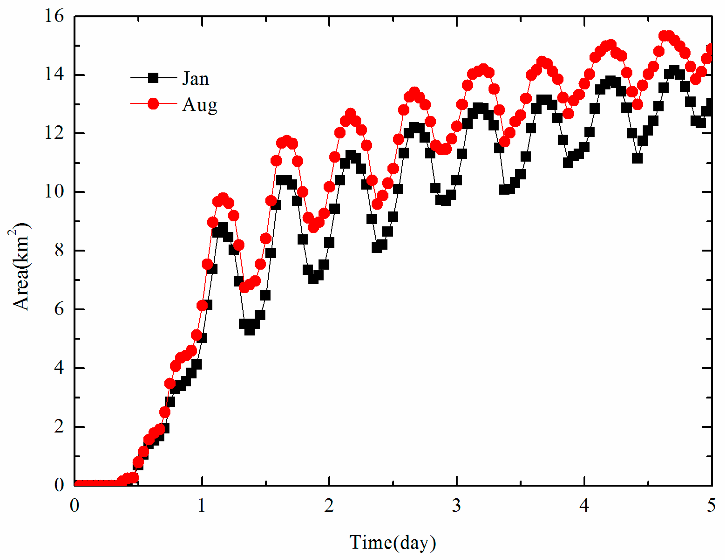
3.5. The Comparison of Two Representative Conditions in the Semi-Closed Bay

In the previous simulations, the profile of temperature and salinity at 18 January is used as background value of Aoshan Bay (Figure 4). To consider temporal variation of the semi-closed bay, the temperature and salinity data at 22 August, which have larger temperature difference, is used as the background value of the simulation. The vertical profiles of temperature and salinity are shown in Figure 14.

By comparing the variation of area where Ra is bigger than 0.002 at artificial upwelling sites 1 in January and August (Figure 15), we can find that artificial upwelling has better performance in August. The larger temperature difference can maintain more artificial upwelling in surface water. Hence, artificial upwelling is more suitable for hot weather, which has larger temperature difference between bottom and surface water. More details could be seen from Figure 16. The basic variations of effect area have a similar pattern for January and August. However, artificial upwelling in August significantly has larger effect area. In conclusion, artificial upwelling is more suitable for strong-stratification condition. However, even when stratification is weak, artificial upwelling can also work with slightly worse performance.

3.6. Discussion of the Limitations of this Study

Firstly, the hindrance of seaweed and algae to the diffusion of artificial upwelling is not considered. Due to the existence of seaweed and algae in the surface water, the water exchange on the surface will be slowed down, which make the spreading velocity of artificial upwelling decrease.

Hence, if we consider the hamper of seaweed and algae, we will find a more significant variation of nutrient concentration in surface water will be more focused at a smaller area. Secondly, the nutrient concentration of overlying water is assumed to be stable. Once we use artificial upwelling to lift the overlying water, the overlying water will be diluted by ambient water. However, in our simulation, the dilution of overlying water is neglected. It will increase the concentration of upwelling plume and make the influence of artificial upwelling more obvious. Thirdly, the sampling point is limited. The cost of sampling is very huge, we carry on three sea trials, but only get surface water at eleven sites and overlying water at three sites. We hope to get more valuable data in the following sea trials.

4. Conclusions

Artificial upwelling is considered a promising way to solve nutrient limitations and stimulate the growth of seaweed. In this study, the appropriate position of artificial upwelling in the semi-closed bay is studied as one key problem of the artificial upwelling’s application. By using FVCOM and considering the effect of spring-neap tide and the running time of artificial upwelling, the researchers find the appropriate position in the semi-closed bay and test artificial upwelling’s performance in alleviating nutrient limitation.

Firstly, the effect of tidal and residual current to artificial upwelling is analyzed. It is found that tidal current has more significant influence to upwelling plume, duo to its relative larger velocity to residual current. Secondly, 12 potential artificial upwelling positions are selected and divided into three parts to test their performance. For the residual current circulation and small tidal current in the western corner, the upwelling plume generated in position 1 will accumulate efficiently as the increase of runtime. After comparing with other positions, position 1 is the best site to accumulate artificial upwelling. Finally, according the background value of Aoshan Bay, the increasing of nutrient concentration is analyzed. The nutrient concentration will increase about 12% and 40%, if upwelling ratio is 0.2. This study can be used to guide the position selection of artificial upwelling and testify the feasibility of the ecological engineering. For the following study, field applications of artificial upwelling are necessary to measure its effects on seaweed. And further study will focus on ecological simulation to predict the effect of upwelling on the growth of phytoplankton and seaweed.

References

1. Heisler, J.; Glibert, P.M.; Burkholder, J.M.; Anderson, D.M.; Cochlan, W.; Dennison, W.C.; Dortch, Q.; Gobler, C.J.; Heil, C.A.; Humphries, E. Eutrophication and harmful algal blooms: A scientific consensus. Harmful Algae 2008, 8, 3–13. [Google Scholar] [CrossRef] [PubMed] [Green Version]
2. Anderson, D.M. Turning back the harmful red tide. Nature 1997, 388, 513. [Google Scholar] [CrossRef]
3. Anderson, D.M. Approaches to monitoring, control and management of harmful algal blooms (HABs). Ocean Coast. Manag. 2009, 52, 342–347. [Google Scholar] [CrossRef] [Green Version]
4. Shi, H.; Zheng, W.; Zhang, X.; Zhu, M.; Ding, D. Ecological–economic assessment of monoculture and integrated multi-trophic aquaculture in Sanggou Bay of China. Aquaculture 2013, 410, 172–178. [Google Scholar] [CrossRef]
5. Jiang, Z.J.; Fang, J.G.; Mao, Y.Z.; Wang, W. Eutrophication assessment and bioremediation strategy in a marine fish cage culture area in Nansha Bay, China. J. Appl. Phycol. 2010, 22, 421–426. [Google Scholar] [CrossRef]
6. Fei, X. Solving the coastal eutrophication problem by large scale seaweed cultivation. In Asian Pacific Phycology in the 21st Century: Prospects and Challenges; Springer: Berlin/Heidelberg, Germany, 2004; pp. 145–151. [Google Scholar]
7. Xiao, X.; Agusti, S.; Lin, F.; Li, K.; Pan, Y.; Yu, Y.; Zheng, Y.; Wu, J.; Duarte, C.M. Nutrient removal from Chinese coastal waters by large-scale seaweed aquaculture. Sci. Rep. 2017, 7, 46613. [Google Scholar] [CrossRef] [PubMed] [Green Version]
8. Forchino, A.; Borja, A.; Brambilla, F.; Rodríguez, J.G.; Muxika, I.; Terova, G.; Saroglia, M. Evaluating the influence of off-shore cage aquaculture on the benthic ecosystem in Alghero Bay (Sardinia, Italy) using AMBI and M-AMBI. Ecol. Indic. 2011, 11, 1112–1122. [Google Scholar] [CrossRef]
9. Ni, Z.; Zhang, L.; Yu, S.; Jiang, Z.; Zhang, J.; Wu, Y.; Zhao, C.; Liu, S.; Zhou, C.; Huang, X. The porewater nutrient and heavy metal characteristics in sediment cores and their benthic fluxes in Daya Bay, South China. Mar. Pollut. Bull. 2017, 124, 547–554. [Google Scholar] [CrossRef]
10. Wang, W.W.; Li, D.J.; Zhou, J.L.; Gao, L. Nutrient dynamics in pore water of tidal marshes near the Yangtze Estuary and Hangzhou Bay, China. Environ. Earth Sci. 2011, 63, 1067–1077. [Google Scholar] [CrossRef]
11. Shi, J.; Wei, H. Simulation of hydrodynamic structures in a semi-enclosed bay with dense raft-culture. Period. Ocean Univ. China Chin. 2009, 39, 1181–1187. [Google Scholar]
12. Williamson, P.; Wallace, D.W.R.; Law, C.S.; Boyd, P.W.; Collos, Y.; Croot, P.; Denman, K.; Riebesell, U.; Takeda, S.; Vivian, C. Ocean fertilization for geoengineering: A review of effectiveness, environmental impacts and emerging governance. Process Saf. Environ. Prot. 2012, 90, 475–488. [Google Scholar] [CrossRef]
13. Lovelock, J.E.; Rapley, C.G. Ocean pipes could help the Earth to cure itself. Nature 2007, 449, 403. [Google Scholar] [CrossRef] [PubMed] [Green Version]
14. Aure, J.; Strand, Ø.; Erga, S.R.; Strohmeier, T. Primary production enhancement by artificial upwelling in a western Norwegian fjord. Res. Vet. Sci. 2007, 34, 77–81. [Google Scholar] [CrossRef]
15. Sato, K.; Sato, T. A study on bubble plume behavior in stratified water. J. Mar. Sci. Technol. 2001, 6, 59–69. [Google Scholar] [CrossRef]
16. White, A.; Björkman, K.; Grabowski, E.; Letelier, R.; Poulos, S.; Watkins, B.; Karl, D. An Open Ocean Trial of Controlled Upwelling Using Wave Pump Technology. J. Atmos. Ocean. Technol. 2010, 27, 385–396. [Google Scholar] [CrossRef]
17. Ouchi, K.; Otsuka, K.; Omura, H. In recent advances of ocean nutrient enhancer “TAKUMI” project. In Proceedings of the Sixth ISOPE Ocean Mining Symposium, Changsha, China, 9–13 October 2005; International Society of Offshore and Polar Engineers: Mountain View, CA, USA, 2005. [Google Scholar]
18. Hand, A.; Mcclimans, T.A.; Reitan, K.I.; Knutsen, Ø.; Tangen, K.; Olsen, Y. Artificial upwelling to stimulate growth of non-toxic algae in a habitat for mussel farming. Aquac. Res. 2015, 45, 1798–1809. [Google Scholar] [CrossRef]
19. Maruyama, S.; Yabuki, T.; Sato, T. Evidences of increasing primary production in the ocean by Stommel’s perpetual salt fountain. Deep Sea Res. Part I 2012, 58, 567–574. [Google Scholar] [CrossRef]
20. Ouchi, K.; Yamatogi, T.; Kobayashi, K.; Nakamura, M. Research and Development of Density Current Generator. J. Jpn. Soc. Nav. Archit. Ocean Eng. 2009, 1998, 281–289. [Google Scholar] [CrossRef] [Green Version]
21. Sato, T.; Tonoki, K.; Yoshikawa, T.; Tsuchiya, Y. Numerical and hydraulic simulations of the effect of Density Current Generator in a semi-enclosed tidal bay. Coast. Eng. 2006, 53, 49–64. [Google Scholar] [CrossRef]
22. Jun, C.J.-F.Z. Distribution and variation of hydrographic factors in the Aoshan Bay. Mar. Fish. Res. 2004, 2, 66–72. [Google Scholar]
23. Lin, T.; Fan, W.; Xiao, C.; Yao, Z.; Zhang, Z.; Zhao, R.; Pan, Y.; Chen, Y. Energy Management and Operational Planning of an Ecological Engineering for Carbon Sequestration in Coastal Mariculture Environments in China. Sustainability 2019, 11, 3162. [Google Scholar] [CrossRef] [Green Version]
24. Chen, C.; Liu, H.; Beardsley, R.C. An unstructured grid, finite-volume, three-dimensional, primitive equations ocean model: Application to coastal ocean and estuaries. J. Atmos. Ocean. Technol. 2003, 20, 159–186. [Google Scholar] [CrossRef]
25. Mellor, G.L.; Yamada, T. Development of a turbulence closure model for geophysical fluid problems. Rev. Geophys. 1982, 20, 851–875. [Google Scholar] [CrossRef] [Green Version]
26. Smagorinsky, J. General circulation experiments with the primitive equations: I. The basic experiment. Mon. Weather Rev. 1963, 91, 99–164. [Google Scholar] [CrossRef]
27. Chen, C.; Cowles, G.; Beardsley, R.C. An Unstructured Grid, Finite-Volume Coastal Ocean Model: FVCOM User Manual; UMASSD Technical Report-06-0602; SMAST: New Bedford, MA, USA, 2006. [Google Scholar]
Figure 1. Overview of experiment site in Aoshan Bay (located at 36°25′45″ N and 120°43′43″ E in Yellow Sea of China). This semi-closed bay has been used for seaweed agriculture.
Water 12 00177 g001
Figure 2. A schematic diagram of air-injection artificial upwelling system, which is mainly consisted of solar platform and air-injection system. The air-injection system is used to generated artificial upwelling at seaweed agriculture area.
Water 12 00177 g002
Figure 3. Model domain of Aoshan Bay. White circles represent the positions of velocity observation stations, which is used to measure tidal current velocity. The depth contour represents the lowest astronomical tides.
Water 12 00177 g003
Figure 4. Vertical distribution of salinity (left) and temperature (right) at observation station 4 of Aoshan Bay at 18 January 2019.
Water 12 00177 g004
Figure 5. Comparisons of model and observed sea elevations at Nv island tidal station.
Water 12 00177 g005
Figure 6. Comparisons of measured and calculated M2 (a) and S2 (b) tidal current ellipses at four stations.
Water 12 00177 g006
Figure 7. Horizontal distributions of residual current measured in numerical simulation for spring tide, shown by the yellow arrows. The percent of sea surface temperature variation caused by artificial upwelling (Ra) after running artificial upwelling for 10 days, shown by contour map. The diffusion area caused by residual current is also marked by the white square.
Water 12 00177 g007
Figure 8. Horizontal distribution of the tidal current at 10:00 a.m. (a) and 15:00 p.m. (b), and the percent of sea surface temperature variation caused by western artificial upwelling at 10:00 a.m. (c) and 15:00 p.m. (d), and the percent of sea surface temperature variation caused by eastern artificial upwelling at 10:00 a.m. (e) and 15:00 p.m. (f) after running artificial upwelling for 10 days.
Water 12 00177 g008
Figure 9. Horizontal distributions of tidal current for ebb tide from the model results (The tidal elevation at the open boundary consisted of four major tidal constituents (M2, S2, K1, and O1) from TPXO in the China Sea with the horizontal resolution of 1/30 degrees.). Red squares represent the positions of artificial upwelling, “1–12” represent the number of artificial upwelling positions. Character “A, B and C” represent three different parts of Aoshan Bay.
Water 12 00177 g009
Figure 10. The variation of area where Ra is bigger than 0.002 for (a) part A contains 1, 5, 6 and 7 upwelling positions. (b) part B contains 2–4 upwelling positions. (c) part C contains 8–12 upwelling positions.
Water 12 00177 g010
Figure 11. (a,d,g,j) represent horizontal distributions of upwelling ratio in surface water at four different times after running artificial upwelling for 5 days in positions 1. (b,e,h,k) represent horizontal distributions of upwelling ratio in surface water at four different times after running artificial upwelling for 5 days in positions 2. (c,f,i,l) represent horizontal distributions of upwelling ratio in surface water at four different times after running artificial upwelling for 5 days in positions 11.
Water 12 00177 g011
Figure 12. A schematic diagram of 11 sampling sites in Aoshan Bay.
Water 12 00177 g012
Figure 13. The relationship between P and DIN concentration and upwelling ratio (Ra).
Water 12 00177 g013
Figure 14. Vertical distribution of salinity and temperature on 22 August at three different times in Aoshan Bay.
Water 12 00177 g014
Figure 15. The variation of area where Ra is bigger than 0.002 at artificial upwelling sites 1 in January and August.
Water 12 00177 g015
Figure 16. (a,c) represent horizontal distributions of upwelling ratio in surface water at two different times after running artificial upwelling for 5 days at site 1 in January. (b,d) represent horizontal distributions of upwelling ratio in surface water at two different times after running artificial upwelling for 5 days at site 1 in August.
Water 12 00177 g016