Hazard Assessment Based on the Combination of DAN3D and Machine Learning Method for Planning Closed-Type Barriers against Debris-Flow


Department of Civil and Environmental Engineering, KAIST, Daejeon 34141, Korea
*
Author to whom correspondence should be addressed.
Water 2020, 12(1), 170; https://doi.org/10.3390/w12010170
Submission received: 31 October 2019
/
Revised: 16 December 2019
/
Accepted: 3 January 2020
/
Published: 7 January 2020
(This article belongs to the Special Issue Debris Flows Research: Hazard and Risk Assessments)
Abstract
:If a slope located near a densely populated region is susceptible to debris-flow hazards, barriers are used as a mitigation method by placing them in flow channels; i.e., flowpaths. Selecting the location and the design of a barrier requires hazard assessment to determine the width, volume, and impact pressure of debris-flow at the moment of collision. DAN3D (Three-Dimensional Dynamic Analysis), a 3D numerical model for simulating debris-flow, has been widely used to perform hazard assessment; however, solely using DAN3D would be both insufficient and inefficient in finding the optimal barrier location. Therefore, the present study developed a framework that interprets the results from DAN3D simulation without considering any barriers. Then, the framework generates hazard assessment maps showing the impact parameters of debris-flow along the flowpath by various algorithms and machine learning methods, such as the k-means clustering algorithm, and also computes the width of the debris-flow, which is not explicitly calculated in DAN3D. A case study of the debris-flow at Umyeon mountain, Korea, in 2011, was used to generate hazard assessment maps. The maps were demonstrated to be a tool to quickly compute the impact parameters for conceptual barrier design with the aim of finding potential barrier locations.
1. Introduction
Debris-flow is a rapid movement of a fluid-like slurry composed of loose soil, rock, organic materials, and water. It is considered as one of the most destructive and dangerous phenomena among landslide disasters, often resulting in property damage and maybe leading to human casualties [1]. Even with an early warning system, a full evacuation in a densely populated region is difficult due to the rapid movement, which leads to a short time-interval between the initiation and arrival of debris flow. With recent trends showing an increase in the frequency of debris-flow occurrence from massive rainstorms caused by climate changes [2], reliable mitigation methods are required against debris-flow.
Closed-type barriers, such as check dams [3], are often designed due to their reliability in effective mitigation against debris-flow. The function of a closed-type barrier is to retain the volume of debris-flow by confining the debris-flow. A barrier is built within a valley or channel to contain the debris-flow using various materials from gabions, soil, stone, concrete, or wood [4]. The barrier should prevent the overflowing and excessive overtopping of the debris-flow. Additionally, the structural integrity of the barrier should be ensured to avoid wall collapse, which may lead to further damage by initiating a debris-flow [5]. To design barriers as an effective mitigation method against debris-flow, the location of the debris-flow flowpath, which is the path on which debris-flows travel, and the characteristic quantities of debris-flow, such as the volume, height, and impact force, at each flowpath location are required.
The parameters of debris-flow can be determined by performing a run-out analysis. Empirical methods use previous debris-flow case studies to generate correlations to estimate the parameters of debris-flow based on other variables. The angle of reach (fahrböschung angle) was used to estimate the volume of the debris-flow [6]. Empirical methods [7,8] used the volume and the volumetric discharge rate of debris-flow to estimate the speed and height of the debris-flow. Although empirical methods are simple and powerful analysis tools, it is difficult to use these methods if there is a lack of a database to generate a reliable empirical statistical correlation. Furthermore, empirical methods cannot determine the flowpath of the debris-flow. Therefore, numerical methods have been widely used to conduct run-out analyses.
Many numerical methods for simulating debris-flow have been developed [6,9], and numerous studies have used these methods to evaluate the performance of barriers, such as check dams. The studies by Osti and Egashira [10] and Remaitre et al. [11] used a numerical method to evaluate the performance of a series of planned check dams. Gregoretty et al. [12] used Geographic Information System (GIS)-based cells to generate reliable evaluation methods for assessing the performance of barriers. The GIS-based cell model method was upgraded by Bernard et al. [13] so that non-erosive surfaces on the concrete bottom of open-type dams can be considered. These studies used case studies of debris-flow to demonstrate the developed numerical methods to assess the performance of planned works. The studies pre-determined the location of the barriers and evaluated their impact. Hence, the performance of barriers might be unsatisfactory due to reasons such as sediments flowing around the barrier or deep erosion from debris-flow, which leads to instability at the barrier foundation [14].
Among the numerical methods for simulating debris-flow, the three-dimensional model Dynamic Analysis (DAN3D) [15], which is a three-dimensional (3D) debris-flow semi-empirical numerical method, has been widely used in recent studies. This method has reliably simulated various run-out case studies, such as the debris-flow at Umyeon mountain in 2011 [16] and the Oso landslide at Oso, Washington, in 2014 [17]. The reason for the versatility of DAN3D can be attributed to its features. On top of the ability to perform 3D simulation, DAN3D allows variation in the soil rheology for different geographical locations. It also incorporates the entrainment phenomenon, which is a crucial component required to simulate the increasing sediment volume as debris-flow propagates [1]. Hence, this study has utilized the DAN3D program for application in barrier design. The theory and governing principles of DAN3D will be introduced in the next section.
Choi et al. [18] showed a usage of DAN3D numerical simulations to design optimal barrier locations. DAN3D simulations were conducted by using a barrier with the same height and thickness but placing it in different locations along the flowpath. The results showed that a smaller barrier would be sufficient to mitigate debris-flow if the barrier is installed near the source. The entrainment phenomenon of debris-flow shows that the volume and the width of debris-flow both increase relative to the distance that the debris-flow travels. However, the placement of the barrier closer to the source increases the risk of global failure safety as the regions may be subjected to landslide failure. As potential landslide regions are often located at high elevation with a steep slope gradient, constructing barriers nearer to the source may pose a challenge.
Additionally, solely using DAN3D might not be sufficient to derive all the required characteristic quantities of debris-flow. The DAN3D does not explicitly compute the width of a debris-flow [19]. A closed-type barrier is useful when the length of the barrier wall is larger than the width of the debris-flow. Therefore, the width of the debris-flow would define the minimum length of the barrier required. DAN3D does not compute this important parameter; hence, an additional analysis is needed.
Besides, it is very time-consuming in DAN3D to compute the loads exerted on a barrier from collisions between a barrier and debris-flow. Several numerical simulations, with each simulation prescribing different barrier locations and different wall designs, would be required. Furthermore, a large number of simulations would be required to have enough confidence in the optimality of the chosen location and design for barriers. Hence, solely using DAN3D simulation may not be an efficient strategy to find the optimal location for barriers.
The inefficiency in barrier design arises from directly performing a detailed performance evaluation for a barrier with a prescribed location and wall dimension. The efficiency in barrier design can be enhanced if the wall dimensions can be roughly estimated at a proposed barrier location based on the characteristic quantities of debris-flow, such as the width, volume, and impact pressure of the debris-flow along the flowpath.
Recently, machine learning methods, such as the artificial neural network (ANN), fuzzy clustering analysis, and genetic algorithm, have been applied to assess performances of structure or soil [20,21,22] and to conduct flood risk assessment [23,24]. The study on flood risk assessment used the combination of GIS and machine learning methods to generate maps that show the level of flood risk of the metro system. Similarly, the present study aims to combine machine learning methods and DAN3D simulation to produce simple hazard assessment maps that display the properties of the debris-flow along the flowpath.
In this study, a framework was developed to extract the results from DAN3D simulation, to interpret the results by using machine learning methods and well-established computer algorithms, and to generate GIS maps showing the characteristic properties of debris-flow. The quantities of debris-flow shown in the generated maps can provide the design parameters required for estimating the barrier wall dimensions. A case study based on the debris-flow hazard at Umyeon mountain in July 2011 was used to demonstrate the applicability of the framework to calculate the properties of debris-flow for any proposed barrier location. Based on this case study, the essential findings and the implications of the results will be discussed.
2. DAN3D
2.1. Governing Equations
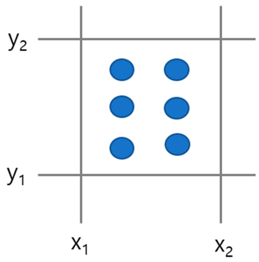
DAN3D is a 3D run-out semi-empirical numerical analysis method developed as an extension of DAN-W [25], a 2D run-out analysis method. The DAN3D method is based on the principle of mass and momentum conservation in continuum mechanics. The debris-flow is modeled as an equivalent fluid [25,26], and a meshless Lagrangian frame of reference is used. To further simplify, the method adopts the depth-averaged velocity and nonhydrodynamic internal stress distribution based on the assumptions developed from research by Savage and Hutter [27]. The initial landslide volume is discretized into N-many particles with an equal amount of volume. The particles are placed evenly on an orthogonal grid, as shown in Figure 1 [15]. The total number of particles in the orthogonal grid is equal to the volume of sliding mass in the grid, which is the product of the area of the grid and the average depth of the soil failure mass, divided by the volume of the individual particle.
The following governing equations of motion [15] are applied to each particle for the debris-flow analysis:
where x and y are the directions parallel and perpendicular to the direction of motion, respectively; is the depth-averaged velocity; ρ is the density of debris-flow; h is the flow depth; g is the gravitational acceleration (9.8 m/s2); k is the stress ratio of lateral stress over bed-normal stress; σz is the bed-normal stress; τzx is the basal resistance, and Es is the growth rate due to entrainment. Smoothed particle hydrodynamics (SPH) [28,29,30] are adopted to simulate the debris-flow from the debris-flow particles. SPH interpolation methods are used to compute the flow depth (h) and flow depth gradient (∇h) in Equations (1) and (2).
2.2. Entrainment
DAN3D incorporates the effect of entrainment, which leads to an increase in volume and a decrease in acceleration. McDougall and Hungr [31] adopted a simple and accurate model for computing the rate of erosion with a growth rate of entrainment (Es), which is defined assuming a natural exponential growth of volume due to entrainment:
where V0 is the initial landslide volume, Vf is the estimated total volume of the landslide exiting the entrainment zone, and S is the average path length that the debris-flow travels. The growth rate (Es) is often computed by performing a back-analysis. A method to estimate the growth rate (Es) based on geotechnical and topological parameters has been proposed in other research [32].
2.3. Rheology
The basal resistance (τzx) is computed based on the rheology of the site. DAN3D currently allows five different rheological models: Newtonian, Plastic, Bingham, Frictional, and Voellmy [15]. The τzx is applied in the direction opposite to the direction of debris-flow motion; hence, it always results in a negative value. In many debris-flow simulations, the Bingham, Frictional, and Voellmy models are commonly utilized. For the case study of this paper, the Bingham model was adopted:
where τyield is the Bingham yield stress, μBingham is the Bingham viscosity, is the depth-averaged velocity in the direction of motion, and h is the depth of debris-flow.
3. Framework
DAN3D models debris-flow as particles; hence, the output of DAN3D simulation computes the XYZ coordinates, volume, depth, and velocity for each debris-flow particle. Then, the characteristic quantities of the entire debris-flow are derived from the interpolated values between the debris-flow particles in DAN3D. The real debris-flow is a continuous mass of fluid-like slurry; hence, the debris-flow particles should be collected together into a cluster to simulate debris-flow as a continuous entity. However, the debris-flow clusters from different landslide regions behave independently from each other; hence, the characteristic quantities of each debris-flow cluster should be derived, instead of combining all the debris-flow clusters as a single entity. An accurate and efficient method was required to sort the debris-flow particles into different groups and to combine the sorted debris-flow particles into different debris-flow particles. Machine learning methods, such as the k-means clustering algorithm, were selected to perform the previously mentioned task.
The developed framework uses the results from DAN3D simulation with the absence of barriers and develops hazard assessment maps using algorithms and machine learning methods. The results of DAN3D were extracted with “parts.txt” and “depth.grd” output files. The file “parts.txt” is a text file that show the properties of debris-flow particles. The file “depth.grd” contains digital elevation model (DEM) data showing the depth of debris-flow. From these DAN3D output files, the XYZ coordinates, volume, depth, and velocity of each debris-flow particle were extracted. From these DAN3D outputs, the generated maps can be used for locating and conducting conceptual design for check dams. The tasks of the framework are broadly grouped into the following categories: (a) determining the state of debris-flow clusters, (b) computing the parameters of an individual debris-flow cluster, and (c) computing the combined parameters of multiple debris-flow clusters at a particular location. The machine learning methods were primarily used to sort the debris-flow particles into different clusters in task (a). Algorithms were used in tasks (b) and (c) to compute the characteristic quantities of debris-flow, including the width of debris-flow, which are not computed in DAN3D simulation. Each task is discussed in detail throughout this section. The overall flowchart of the framework is shown in Figure 2.
3.1. State of Debris-Flow Clusters
The first part of the framework determines the state of the debris-flow by grouping each debris-flow particle into a cluster based on their proximity to each other. A group of debris-flow particles that behaves as a single continuous mass is defined as a debris-flow cluster. The state of a debris-flow cluster refers to the travel direction, location, and boundary of a debris-flow cluster. The framework tracks the change in the state of debris-flow clusters throughout the numerical analysis to define the flowpaths of debris-flows. The flowpath indicates the series of locations where a debris-flow cluster traveled. Barriers, such as check dams, should be placed at locations where the debris-flow clusters would flow. Therefore, the location marked by the flowpath can be used to find potential locations to construct barriers.
3.1.1. Classification of Debris-Flow Particles into Clusters
The positions of debris-flow particles at every simulation time-interval are extracted from DAN3D. Real debris-flow consists of a continuous mass of rock, sediments, and water; hence, the particles are collected together into a cluster to transform the particles into a continuous entity. Therefore, the particles were grouped by classifying them into different clusters, which are the landslide regions that lead to debris-flow. Thus, a machine learning algorithm was adopted to perform classification. Among the machine learning algorithms, the k-means clustering algorithm was selected for its efficiency at sorting particles into different source regions.
The k-means clustering algorithm [33] is an unsupervised machine learning algorithm that aims to partition the uncategorized data points into k-many clusters. The k-means clustering algorithm aims to find the k-many clusters that produce the minimum value of the within-cluster sum of squares (WCSS):
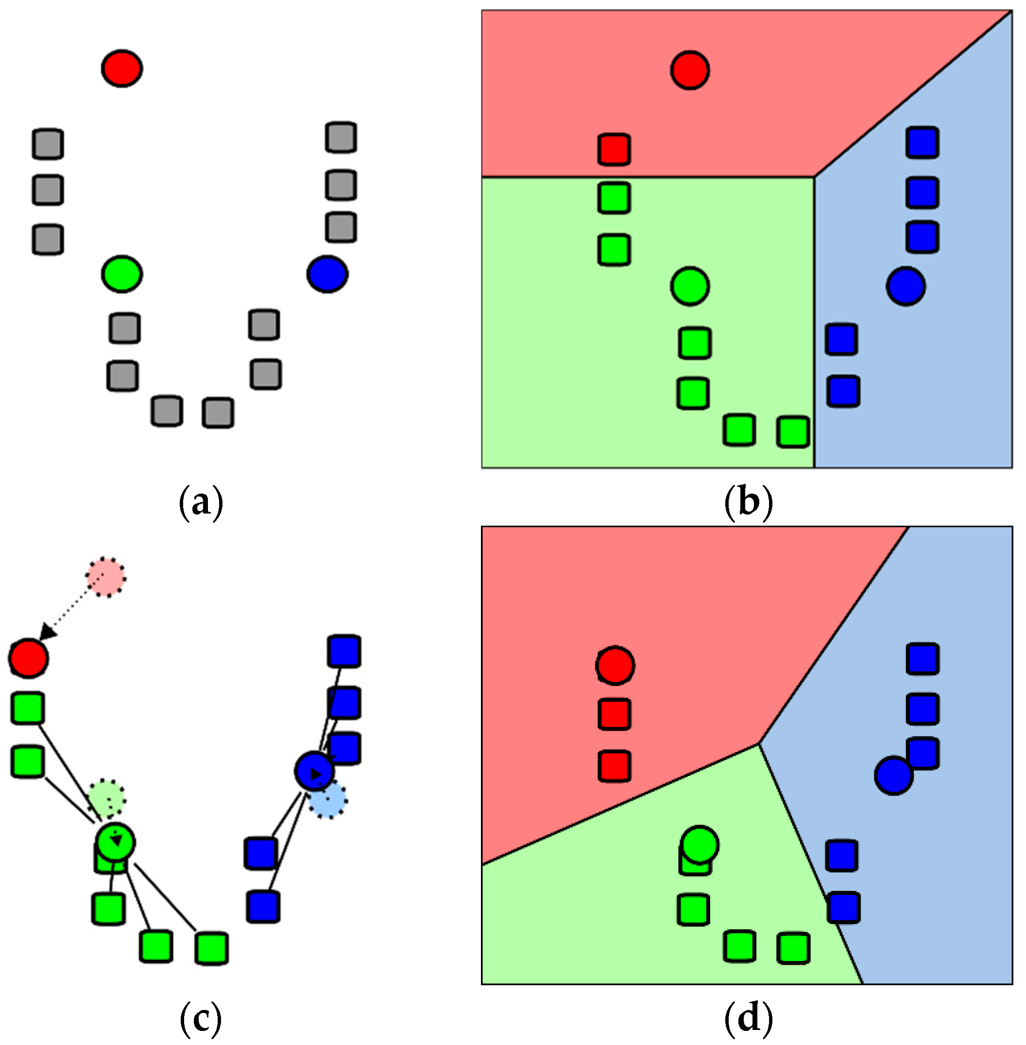
where k is the total number of clusters; n is the total number of points classified to cluster j, xc,j, yc,j are the x- and y-coordinates of the centroid point of cluster j; and xi,j, yi,j are the x- and y-coordinates of data points classified to cluster j. The k-means clustering algorithm generally follows these procedures, as shown in Figure 3:
- Partition: Based on the centroid points, the Voronoi diagram [35] is drawn to partition every data point. The partitioning lines are the midway between the centroid points of different clusters.
- New centroid: A new centroid is computed from the data points using Equation (6).
- Stopping Criterion: Step 2 and 3 procedures are repeated until the minimum value of WCSS is reached.
In order to enhance the accuracy and reduce the number of iterations, the k-means++ algorithm was used in the initialization procedure. The k-means++ algorithm provides initial centroid points that are relatively closer to the optimal centroid points that give the minimum WCSS, compared to centroid points generated from a random procedure. The centroid of a cluster is defined as the average location of the debris-flow particles to define a representative position of a debris-flow cluster:
where xc, yc are the x- and y-coordinates of the centroid of a cluster; xp, yp are the x- and y-coordinates of debris-flow particles classified in the cluster; and n is the number of particles within the cluster.
However, the main limitation of using the k-means clustering algorithm is that the value of k, which expresses the total number of clusters for our analysis, needs to be prescribed. The user can manually assign the initial k value, which is the number of landslide sources when the time step is equal to zero (0); i.e., the initial stage. In this framework, we suggest using the Elbow method [37], which automatically detects the optimal value of k for a given layout of data points.
In this study, the k-means clustering function in the scikit-learn Python library [38] was utilized. The inputs required for implementing the k-means clustering algorithm are the total number of different landslide sources and the x- and y-coordinates of the debris-flow particles at the initial simulation condition; i.e., when the time step is equal to zero (0). The combination of the k-means clustering algorithm and the Elbow method can find the number of sources automatically, compute the centroid of each cluster, and classify the debris-flow particles into different debris-flow clusters for any general cases.
3.1.2. Integration of Debris-Flow Particles into a Debris-Flow Cluster
Each debris-flow cluster is a collection of debris-flow particles; therefore, we can assume that the behavior of the entire debris-flow cluster is the cumulative behavior of individual debris-flow particles. However, assessing every debris-flow particle becomes more complex as the number of debris-flow particles increases. Furthermore, it may not be suitable to account for every debris-flow particle in certain computations, such as computing the outer extent of a debris-flow cluster. Accordingly, the behavior of the entire debris-flow cluster can be assessed using the centroid and the boundary of the cluster, which can be used to track the changes in the location and size of a debris-flow cluster, respectively. This simplification provides computational benefits by reducing the computational load while maintaining its relevant information to provide accurate results.
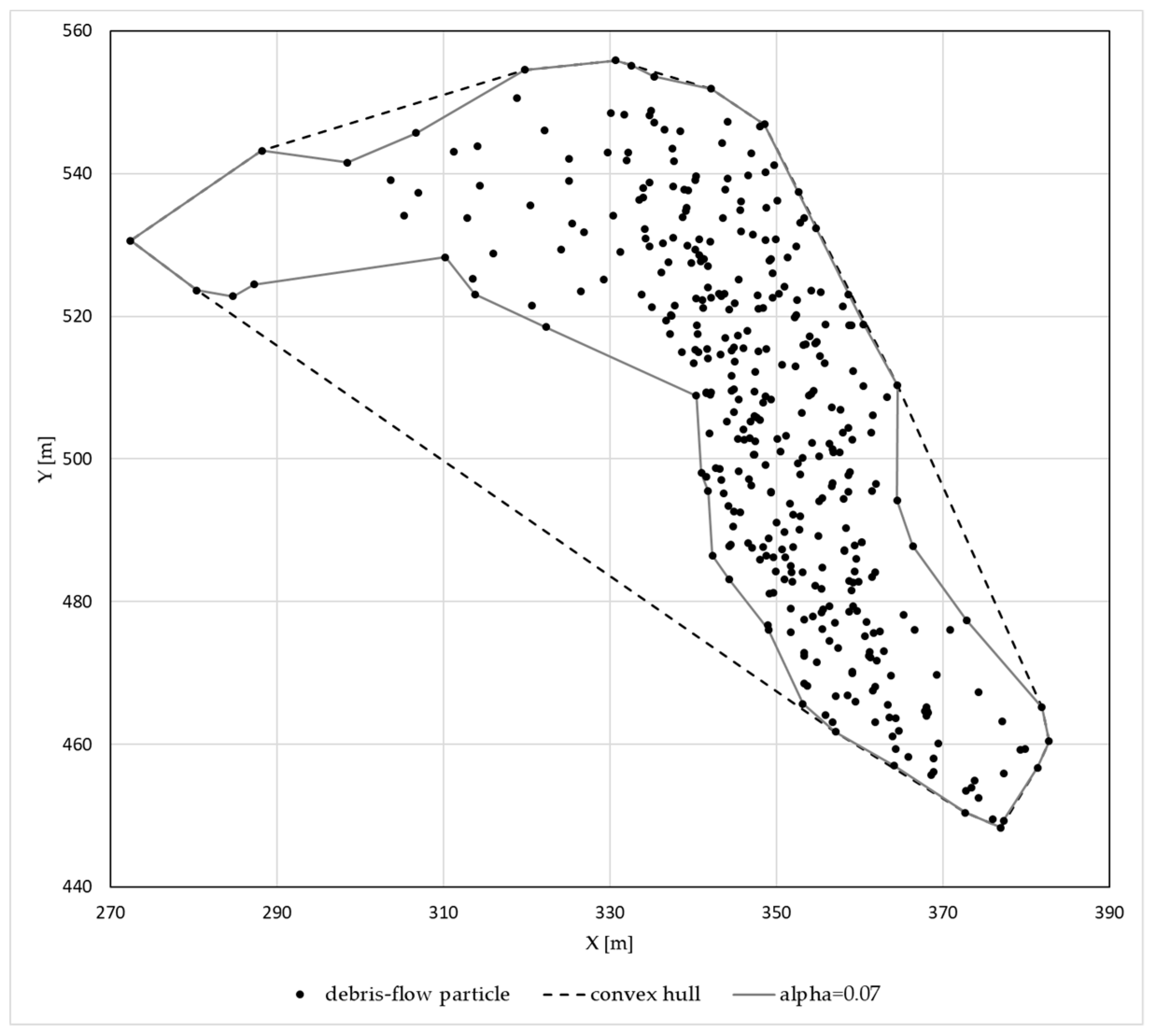
The centroid of the debris-flow cluster is computed using Equation (6). The boundary of a debris-flow cluster can be defined as a set of debris-flow particle locations that indicate the extent of the cluster. The α-shape (alpha-shape) [39] algorithm is used to search for the boundary of a debris-flow cluster. The α-shape is a generalized solution to the Convex Hull problem [40]; therefore, the polygon formed by the boundary points computed by the α-shape algorithm can have a concave shape, unlike the Convex Hull. If the debris-flow particles are distributed as shown in Figure 4, the boundary polygon formed by the α-shape algorithm produces a more accurate boundary compared to the boundary polygon from the Convex Hull algorithm. However, the α-shape algorithm requires a predetermined factor α to compute the generalized disk of the radius (1/α), which describes the radius and curvature of the boundary that connects two boundary points. A simple algorithm has been developed to find an optimal value for factor α, which will be described in Appendix A.
A modification of the α-shape algorithm was implemented with Python3 code, which inputs the data points, and a single parameter that considers the Convex Hull and α-shape. The code was based on the Concave Hull algorithm developed by Kevin Dwyer [41].
3.1.3. Interaction between Debris-Flow Clusters
The centroid and boundary of a debris-flow cluster track the changes in the state of a debris-flow cluster. These changes are caused by a combination of phenomena, such as lateral spreading, deposition, and entrainment, as the debris-flow cluster flows along the topography of the mountain. Entrainment and deposition are simulated through 3D debris-flow numerical analysis by making assumptions and applying mechanics.
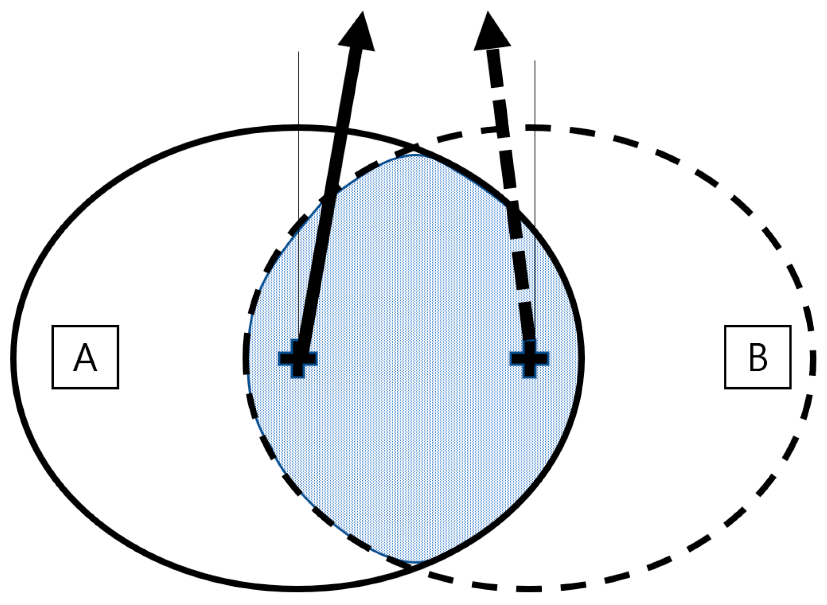
Besides, the merging and splitting of the debris-flow clusters also changes the state of the debris-flow cluster. For example, if landslides occur in two different regions that are close to each other, the debris-flow clusters may merge as they flow into the same location. Therefore, the merging and splitting of debris-flow clusters would significantly affect the state of the debris-flow clusters. Criteria have been set to determine the merging and splitting of debris-flow clusters. Both of the following criteria need to be satisfied in order for clusters to be considered as merging (Figure 5):
- Travel direction: The difference in the travel directions of the debris-flow clusters must be within a tolerance limit of 10°.
- Overlapping ratio: The ratio between the number of debris-flow particles located inside the boundary of another cluster over the total number of debris-flow particles in the reference cluster needs to be equal to or larger than 0.5.
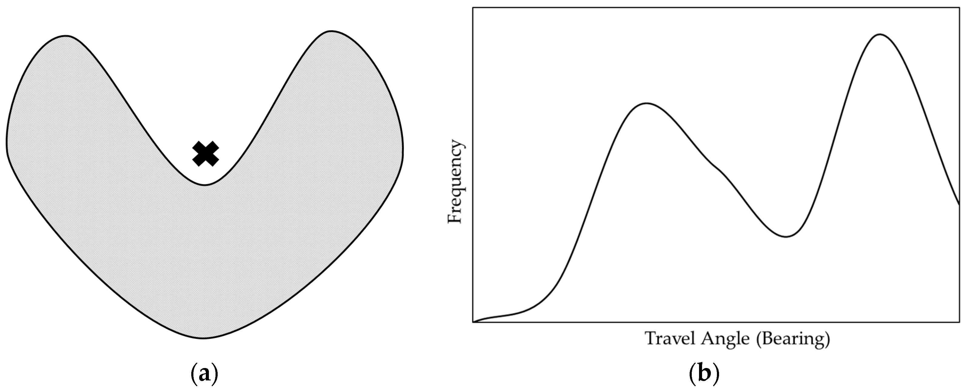
Similarly, both of the following criteria need to be satisfied to determine that a debris-flow cluster is splitting (Figure 6):
- Centroid position: The centroid of the debris-flow cluster must be outside the boundary of the debris-flow cluster.
- Travel angle peaks: A frequency distribution plot displaying the travel direction of debris-flow particles in a cluster must show more than one distinctive peak.
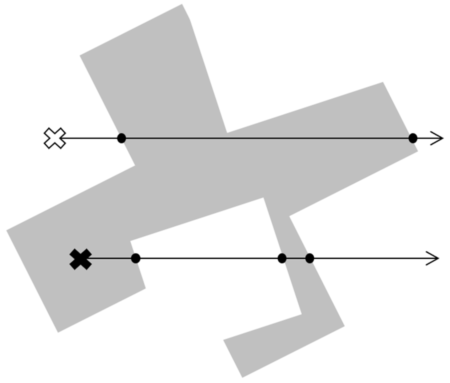
Both the overlapping and centroid position criteria need to determine if a debris-flow particle is inside the boundary of the debris-flow cluster. Such a problem is called a point-in-polygon problem in mathematics. The even–odd rule algorithm [42] is used to solve this problem. The algorithm draws a ray in any fixed direction that starts from a point, and then it counts the amount of time that the ray intersects with the edges of the polygon. If the number of intersections is odd, the point is located inside the polygon and vice versa.
A simple application of the even–odd rule algorithm is shown in Figure 7 to determine whether a point is outside or inside a polygon, which is defined by the grey-shaped region. The points marked by a white cross and a black cross indicate points that are outside and inside the polygon, respectively. Two eastward-heading rays are drawn starting from each point. The rays starting from the white cross and the black cross intersect with the boundary of the polygon twice and trice, respectively. According to the even–odd rule algorithm, the white cross and the black cross are determined to be outside and inside the polygon, respectively.
3.2. Parameters of a Single Debris-Flow Cluster
The state of the debris-flow cluster is derived from integrating individual debris-flow particles into a single unit; i.e., a cluster. Therefore, it produces properties that can only be attributed to the cluster, and some of the properties cannot be computed when analyzing individual debris-flow particles. These emergent properties are the travel direction, width, volume, and impact pressure of debris-flow clusters. Among these emergent properties, the width and volume of a debris-flow cluster provide the dimensional specifications required for designing barriers. For example, the purpose of a closed-type barrier would be to contain the debris when a hazard occurs. Therefore, engineers would need to design the width and height of barriers that can contain the volume of debris-flow clusters and not allow flow around the barrier. In this section, the assumptions and algorithms implemented to derive the emergent properties of a debris-flow cluster are discussed.
3.2.1. Cluster Movement Direction
Although the movement direction of each debris-flow particle may have some variance, the interaction between the particles results in an average movement direction of the debris-flow cluster. The direction of movement for debris-flow clusters is measured by the changing position in the centroid of the debris-flow cluster. The centroid is considered as a representative quantity for the location of the debris-flow cluster. The centroid of a debris-flow cluster within a time interval is assumed to translate linearly for a very short amount of the time-interval. Therefore, a ray that starts from the initial centroid location to the location of the next centroid is drawn to indicate the direction of movement. The direction of the ray—i.e., the travel direction of the debris-flow cluster—is represented by the angle (θ) relative to the eastward direction, which is similar to the definition of angle of polar coordinates:
where Δx and Δy are the differences in debris-flow cluster centroid coordinates in the x- and y-directions, respectively.
3.2.2. Cluster Width
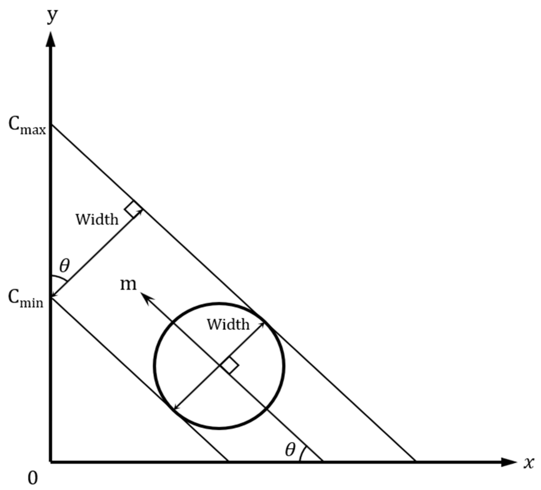
The width of the debris-flow cluster is an important parameter to consider when designing barriers. If the barrier is not a deflection-type barrier, the orientation for the length of the barrier can be assumed to be perpendicular to the direction of the debris-flow. Therefore, the effective width for a debris-flow cluster is considered to be the maximum width of the debris-flow cluster that is perpendicular to the direction of the debris travel direction.
Using the angle (θ) that defines the direction of the debris-flow cluster movement, a linear line is drawn on the boundary defined by the position of the boundary debris-flow particles. The maximum difference in the y-intercept value notes the boundary lines that are furthest from each other, as shown in Figure 8. If the travel direction is parallel to the north direction, the width is computed from the range of the boundary point x–coordinates. Using simple trigonometry, we can compute the effective width of the cluster using
where x and y are the x- and y-coordinates of the boundary points, θ is the angle of the travel direction of the debris-flow cluster, {x} is the set containing the x-coordinates of the boundary points, and {c} is the set containing the y-intercept values calculated by Equation (8).
3.2.3. Cluster Volume
As previously described, DAN3D discretizes the mass of landslide into particles. For SPH interpolation, the volume of debris-flow particles is tracked through the simulation. Therefore, the total volume of a debris-flow cluster is the summation of the volume of the individual debris-flow particles:
where n is the number of debris-flow particles in a cluster, Vi is the volume of each debris-flow particle in the cluster, and Vcluster is the volume of the cluster.
3.2.4. Impact Pressure
The debris-flow is assumed to behave like a fluid—i.e., following the equivalent fluid method [25,26]—therefore, the load applied to a surface by a debris-flow cluster can be quantified by the impact pressure. The impact pressure applied to a surface by a debris-flow is distinguished between a dynamic debris-flow, which refers to a debris-flow with movement, and a static debris-flow, which refers to a deposited debris-flow that shows no movement.
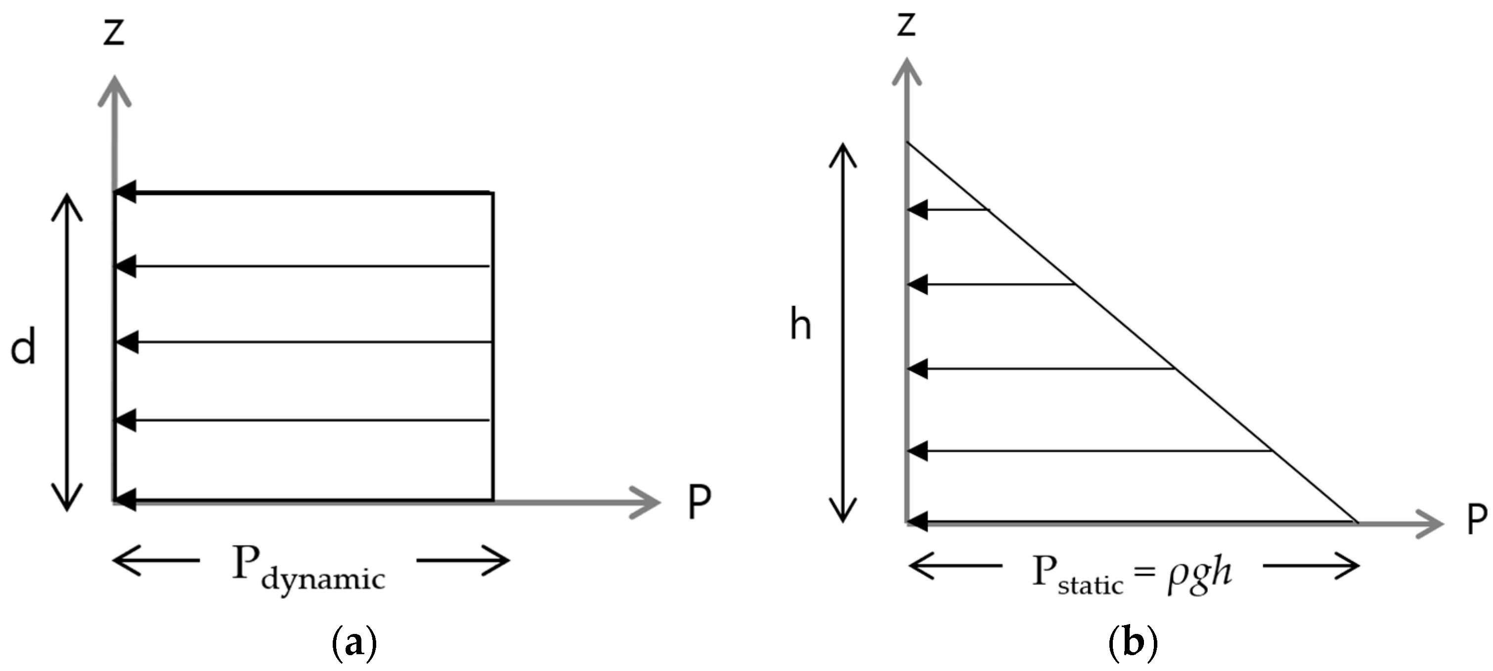
For a dynamic debris-flow, the velocity along the depth of the debris-flow is often considered to be in a full basal condition [15]; therefore, the pressure gradient on a surface from a dynamic debris-flow is assumed to be a constant. The pressure of a dynamic debris-flow is defined by the following equation [43,44]:
where ρdf is the density of the debris-flow, g is the gravitational acceleration (9.8 m/s2), d is the depth of the dynamic debris-flow, and v is the velocity of the debris-flow. Previous research shows that the density of a debris-flow varies from 2000 to 2200 kg/m3 [45].
For a static debris-flow, the debris-flow can be assumed to be in a hydrostatic condition; therefore, the pressure applied by the debris-flow is considered to be linearly increasing with depth. The pressure applied by the static debris-flow along the depth of the debris-flow can be defined as the following:
where h is the depth of the static debris-flow. The pressure gradients of the dynamic and static debris-flows are shown in Figure 9.
Pstatic = ρdfgh,
3.3. Combined Parameters of Multiple Debris-Flow Clusters
If there is more than one landslide source, a barrier may be expected to mitigate the effect of multiple debris-flows. As previously discussed, different debris-flow clusters can merge if the clusters occupy the same location as they flow along the same flowpath. If two debris-flow clusters merge, they start to behave as a single debris-flow cluster. Hence, the parameters of merged debris-flow clusters, which are computed using the previously described algorithms, need to be considered for designing a barrier.
Alternatively, multiple debris-flow clusters can collide against a barrier in succession. Consider debris-flow clusters that are flowing along the same flowpath but do not merge as they do not occupy the same location; the presence of a barrier in the flowpath results in collisions between a debris-flow cluster and the barrier occurring one after the other. Each succession of debris-flow collision provides a new set of parameters of debris-flow that needs to be considered for designing the barriers. This section of the framework describes the method applied to decide the combined parameters of multiple debris-flow clusters that collide against a barrier in succession.
3.3.1. Combined Geometric Parameters: Critical Width and Combined Volume
The collision of multiple debris-flow clusters against a barrier leads to the piling of debris-flow clusters because each debris-flow cluster is deposited in the same region behind the barrier. Each subsequent collision of debris-flow increases the volume of debris-flow deposited at the barrier. Therefore, the combined volume of multiple debris-flow clusters is the sum of the volume of each debris-flow cluster deposited behind the barrier:
where Vcombined is the combined deposited volume, and Vi is the volume of the individual debris-flow cluster that collides against the barrier.
Vcombined = ΣVi,
Unlike the combined volume, the critical width of multiple debris-flow clusters is not a sum of individual widths from each debris-flow cluster. For the first collision between a debris-flow cluster and the barrier, the collided debris-flow will be deposited. The subsequent debris-flow clusters will slide over the deposited debris-flow cluster and collide into the barrier. Therefore, it is reasonable to assume that subsequent debris-flow clusters do not join with the deposited debris until the debris-flow clusters dissipate their kinetic energy; i.e., the velocity becomes zero (0). The critical width from multiple debris-flow clusters is determined by assessing the width of each debris-flow cluster that collides against the barrier. The following equation is used to compute the critical width:
where wcritical is the critical width and {wi} is the set containing the width of the debris-flow clusters that collide against the barrier.
wcritical = max({wi}),
3.3.2. Combined Load Parameters: Impact Load and Moment
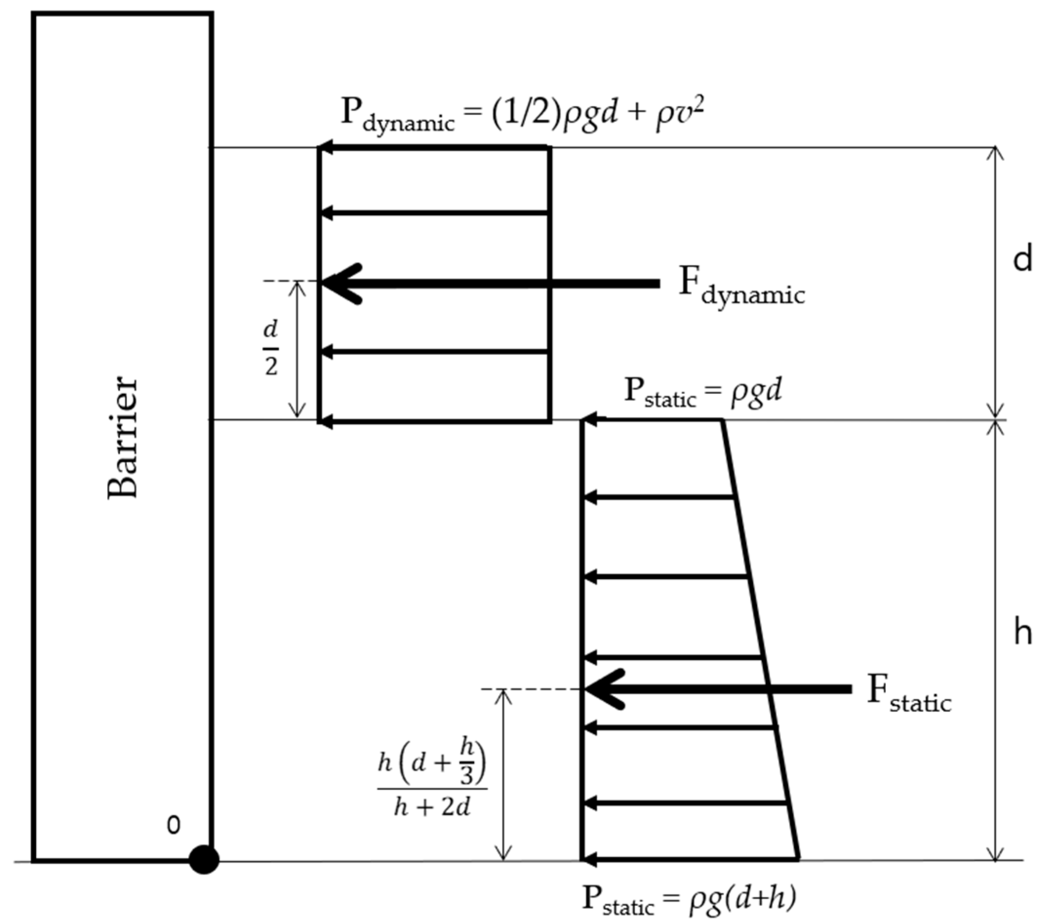
The collision of debris-flow clusters in succession would produce a stacking of multiple debris-flow clusters on top of the previous collision. The first debris-flow cluster collides into the barrier and then gets deposited as it loses its kinetic energy. The deposited debris at the barrier is considered as a static debris-flow. The subsequent debris-flow cluster collision will flow over the deposited debris and collide into the barrier. Therefore, the overall impact pressure of the debris-flow against the barrier would be a combination of the dynamic and static debris-flow clusters, as shown in Figure 10. Similar methods to calculate the overall impact pressure have been developed by Kwon [46], Hübl et al. [47], and Rossi and Armanini [5]. If there is a layer of dynamic debris-flow flowing above a static debris-flow, the depth of the dynamic debris-flow is used to compute the hydrostatic pressure of the static debris-flow.
The overall impact pressures are used to compute the impact load and moment applied to the barrier. The area of the collision between the barrier and a debris-flow cluster is defined as the product of the width and the average depth of a debris-flow cluster. The impact load and moment exerted on the wall due to the debris-flow clusters are computed by
where F is the impact load, M is the impact moment about the pivot point O, d is the depth of a dynamic debris-flow cluster, v is the velocity of a dynamic debris-flow cluster, h is the height of the static debris-flow deposited on the base of the wall, and w is the width of the debris-flow cluster.
4. Results and Discussion
The developed framework was demonstrated using the case study of debris-flow hazard at Umyeon mountain, Seoul, Korea, in 2011, by producing hazard assessment maps, which show the parameters of debris-flow along the flowpaths. Based on DAN3D simulation without the presence of any barrier, the hazard assessment maps were used to calculate the impact parameters of a potential location for closed-type barriers. The findings from the results are discussed.
4.1. Case Study: Umyeon Mountain, Seoul, Korea in 2011
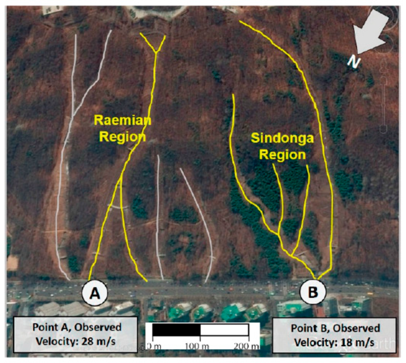
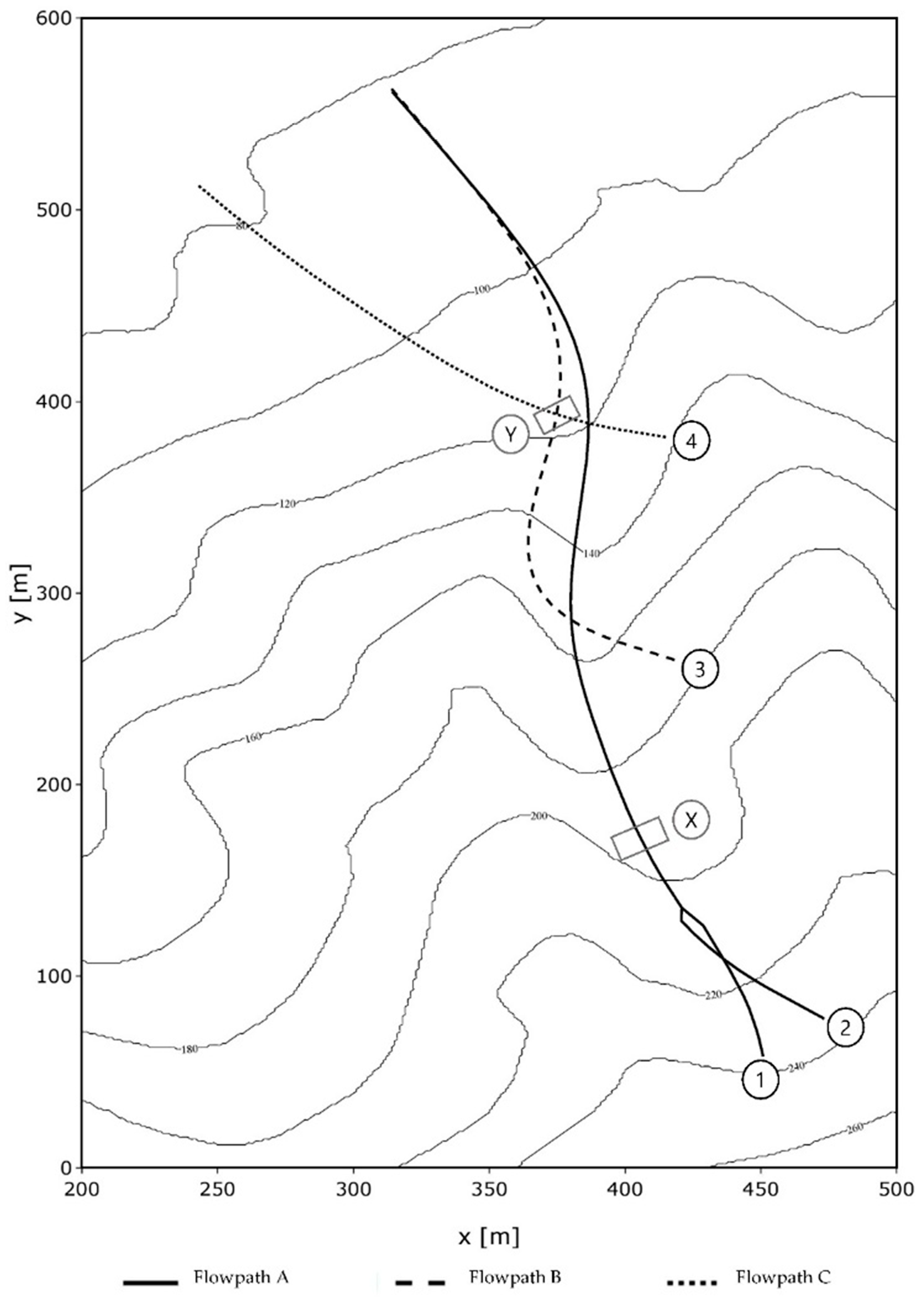
In 2011, a total of about 150 landslides occurred around Umyeon mountain after a continuous rainfall, with a maximum recorded amount of 370 mm. Most of the landslides were mobilized into debris-flow, which led to 16 human casualties and damage to 116 buildings surrounding the mountains [48]. One of the regions around Umyeon mountain that was affected by debris-flow is called the Raemian region. Figure 11, which is a satellite image of Umyeon mountain after the debris-flow hazard, highlights four different landslides that led to the debris-flow that affected the Raemian region. Furthermore, the image shows a flowpath that joins and splits, as shown by the yellow lines in Figure 11.
The observed velocity at the base of Umyeon mountain was recorded as 28 m/s [16], which is around 100 kph; hence, there would have been little or no time for the evacuation for the people in the Raemian region. The usage of barriers would have been suitable as a mitigation method against the debris-flow for this region. Hence, this study selected the debris-flow that affected the Raemian region to demonstrate the applicability of the developed framework by producing hazard assessment maps for designing barriers.
4.2. Inputs and Assumptions for DAN3D
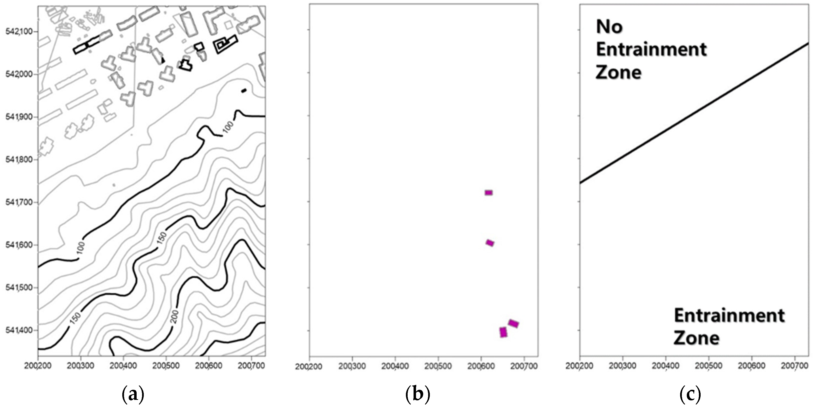
The inputs required for DAN3D for the Raemian region are summarized in Figure 12 and Table 1. DAN3D requires the following three DEM maps: the path topography, which shows the slope topography; the initial source, which shows the location and depth of landslide mass; and the erosion map, which shows the distribution of different soil types. These DEM maps use the surfer grid files format (“*.grd”) generated from Surfer by Golden Software, Inc. (Colorado, USA). The total number of landslide sources was four, as shown in Figure 12b.
The input parameters listed in Table 1 are based on the site investigation report [49] and results from a back-analysis performed using DAN3D [16]. The back-analysis determined the Bingham rheological soil condition at the moment of failure by comparing between the DAN3D simulation results with observed data. The density of the debris-flow was assumed to be 2000 kg/m3 based on a typical density of debris-flow [45].
One of the notable assumptions used in the back-analysis was the simultaneous occurrence of landslides. It is often difficult to determine the chronological sequence of occurrence for the four sources; therefore, it has been assumed that all the landslides occurred simultaneously [16]. Another notable assumption was the soil rheology parameters for the residential Raemian region. As the Raemian region was a residential complex, the region was assumed to be paved with asphalt and concrete at which no soil erosion can occur. Therefore, it was assigned as a “no entrainment zone”, with a value of erosion growth rate equal to zero (0). Although the resistance between the soil-to-soil surface and soil-to-structure interface is different, the difference has been assumed to be negligible. Therefore, the same Bingham model rheology parameters, as shown in Table 1, were assumed for the “entrainment zone” and “no entrainment zone.”
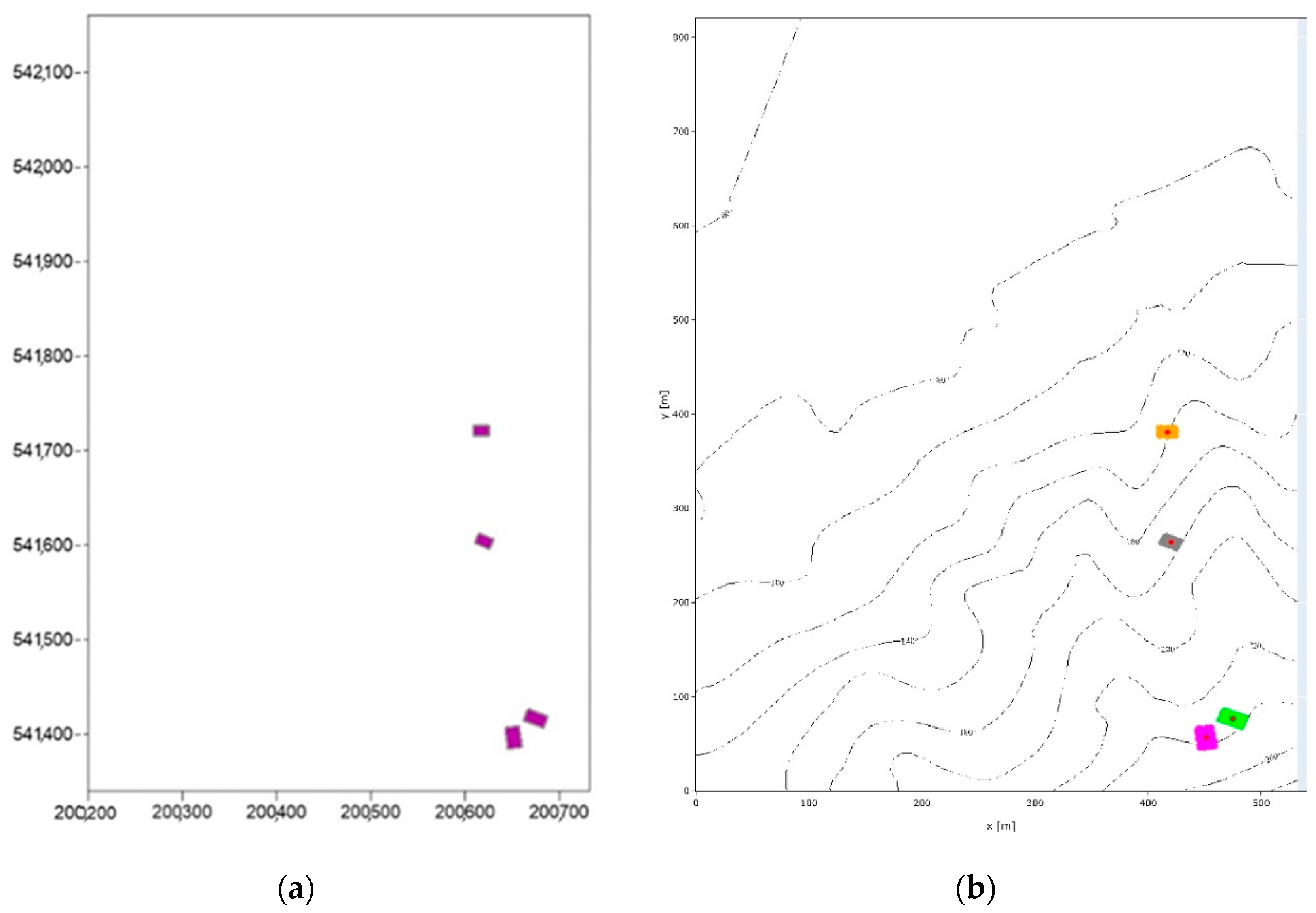
4.3. Verification of K-Means Clustering Algorithm
The combined method of the k-means clustering algorithm and the Elbow method was verified by comparing the result with the initial landslide regions, as shown in Figure 13. The accuracy of the Elbow method is verified by correctly determining the total number of different landslide regions, which is four in our case study. Furthermore, Figure 13b shows that the k-means clustering algorithm has correctly sorted the debris-flow particles into different landslide regions, as shown in Figure 13a. The authors believe the accuracy justifies the using of the k-means clustering algorithm and the Elbow method in the developed framework.
4.4. Hazard Assessment Maps
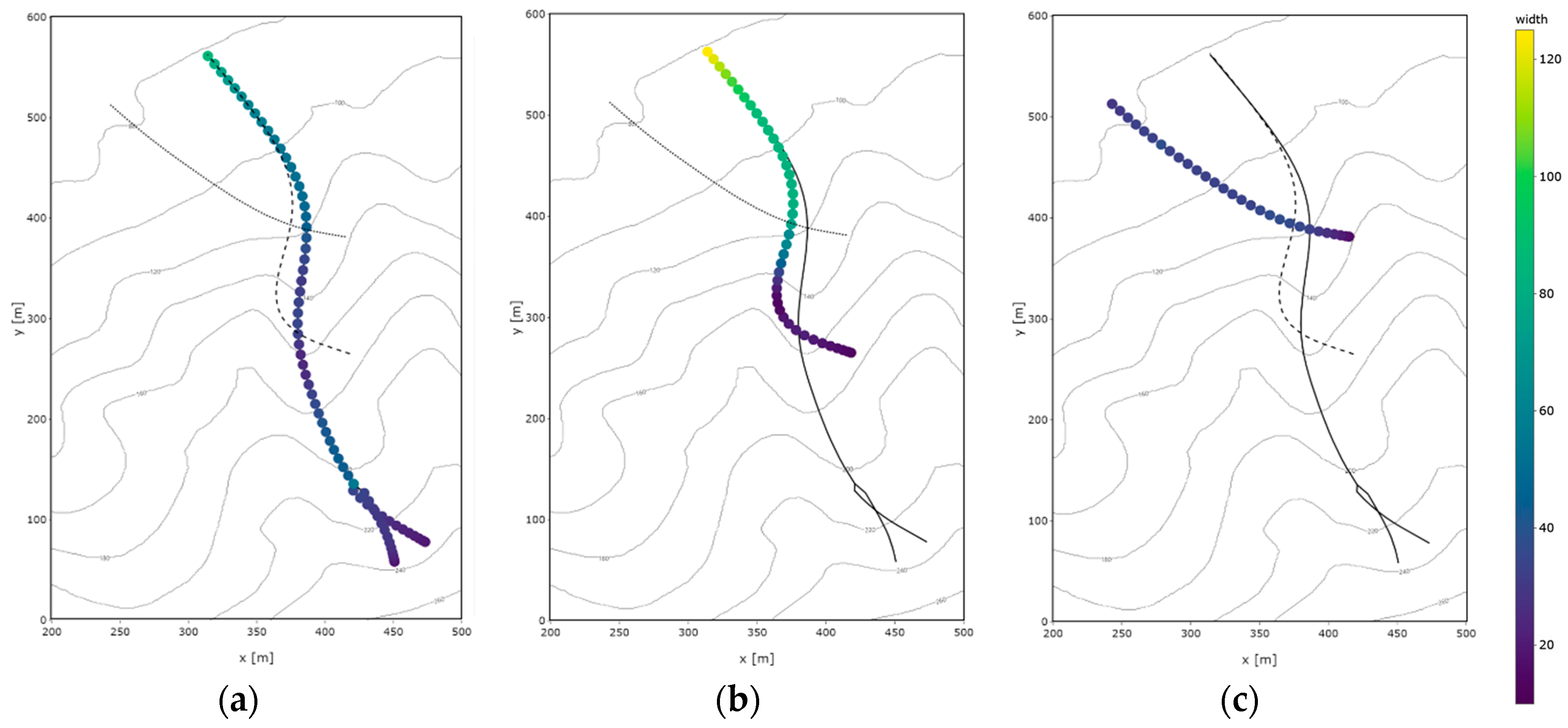
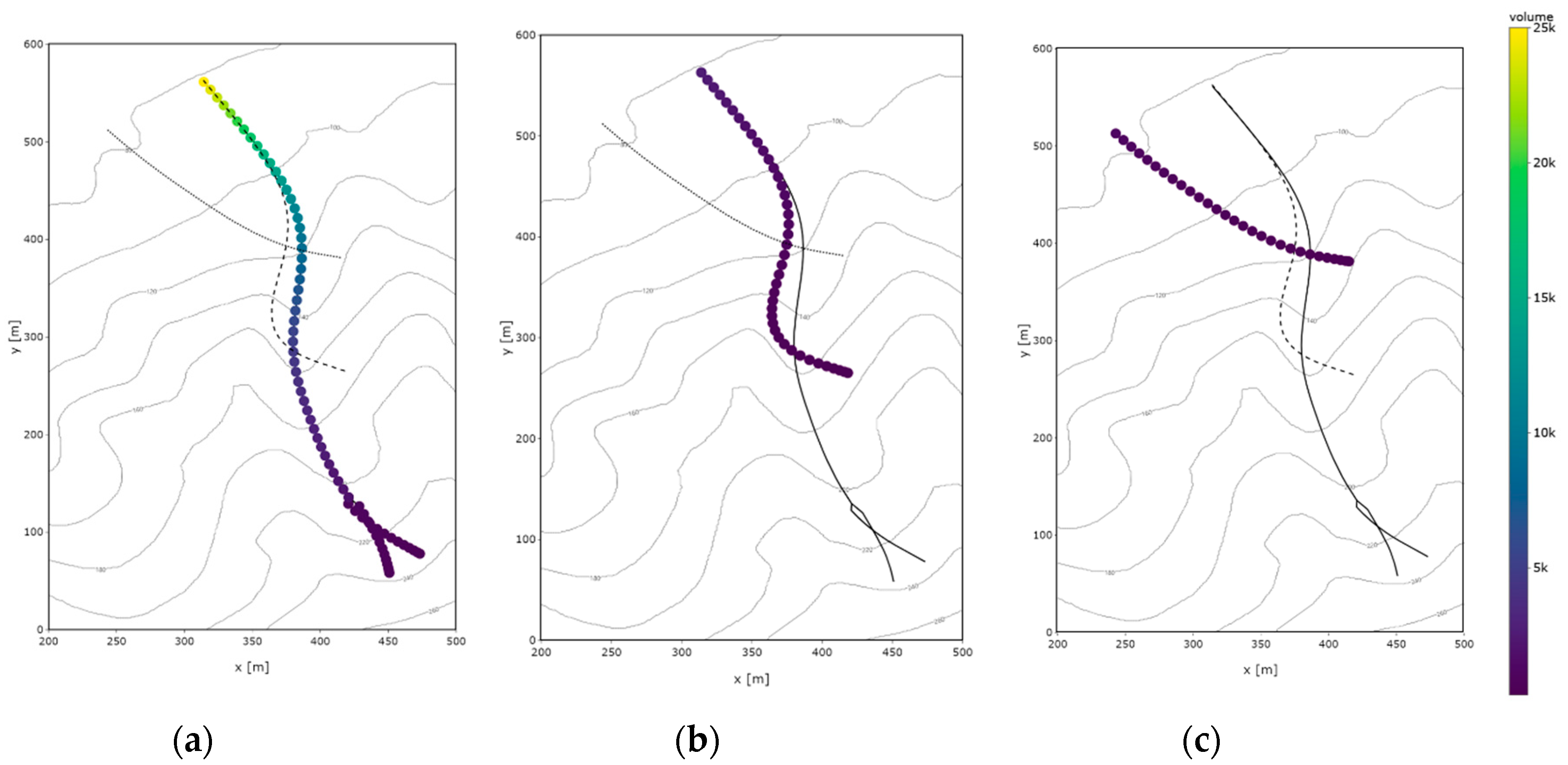
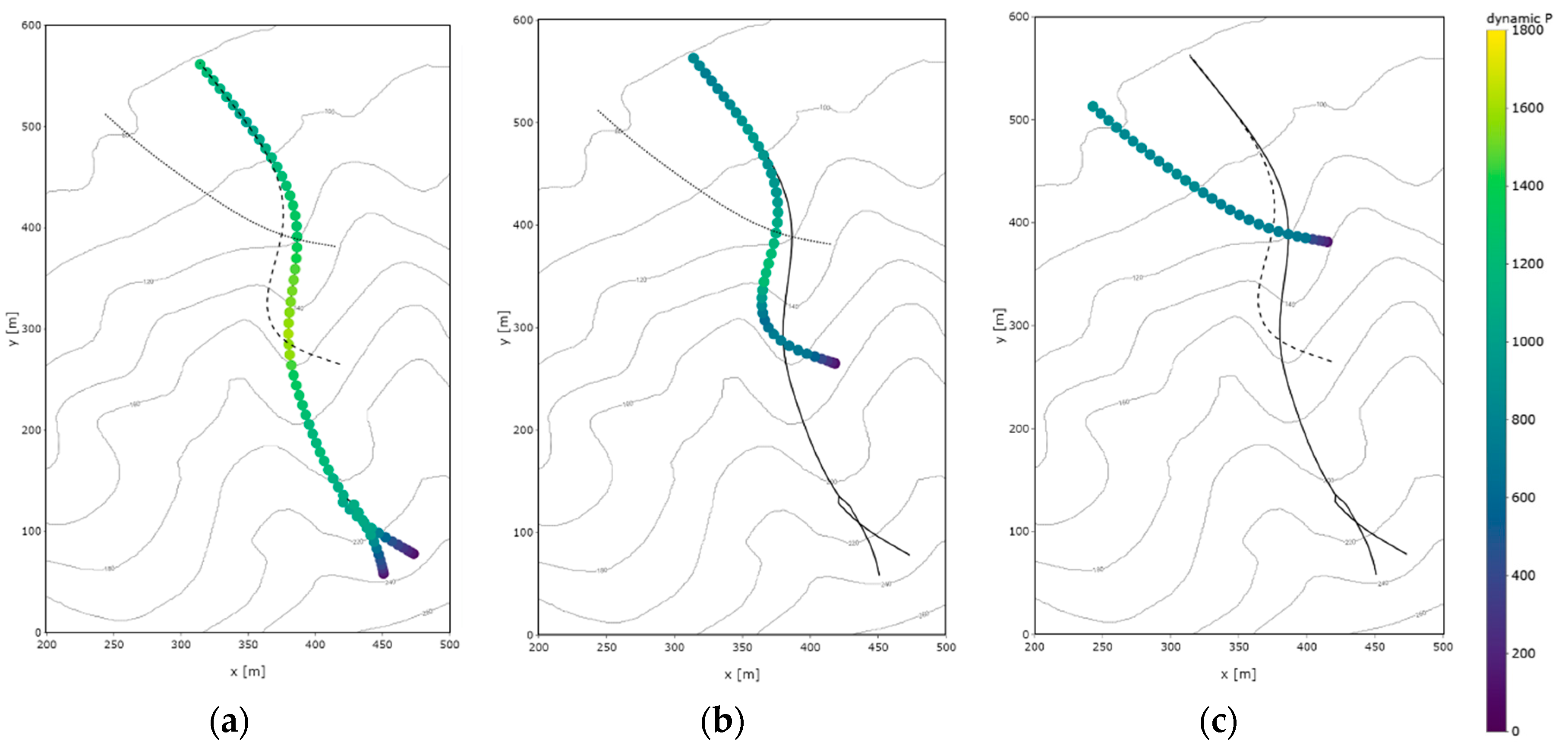
The developed framework processed the results from DAN3D simulation and produced hazard assessment maps that show the parameters of debris-flow along each flowpath, as shown in Figure 14, Figure 15, Figure 16 and Figure 17. The dot points in Figure 15, Figure 16 and Figure 17 show the centroids of the debris-flow clusters recorded at each simulation time.
Figure 14 indicates some notable findings. Firstly, the debris-flow clusters from the first and second source locations merge along flowpath A. Secondly, the debris-flow cluster that flowed along flowpath C had no interaction with other debris-flow clusters. Thirdly, flowpaths A and B converge as they reach the base of the mountain; however, debris-flow clusters from each flowpath did not merge. The observed findings can be explained by the assumption that all the landslides occurred simultaneously. Due to this assumption, the debris-flow clusters located further away from the base of the mountain takes a longer time to reach the base of the mountain. Hence, the debris-flow clusters from flowpath A reach the convergence point at a later time compared to the debris-flow clusters from flowpath B. As the merging criteria specify that two debris-flow clusters occupy the same geographical location, the debris-flow clusters from flowpaths A and B do not merge. Therefore, any debris-flow analysis that uses the assumption of simultaneous landslide occurrence would most likely need to consider the impact parameter from multiple collisions of debris-flow clusters in succession against a barrier.
Figure 15 confirms that the width of the debris-flow clusters increases as the flowpath reaches the base of the mountain. The topography near the base of the mountain would be a relatively flat plane terrain. The debris-flow, which was confined by the shape of the mountain channels, gains the degree of freedom to spread laterally on the flat terrains. The analysis reveals that the width of the debris-flow can reach up to about 125 m. Therefore, an optimal barrier would most likely be a narrow channel or valley in the mountains to avoid designing an excessively long wall.
Figure 16 also assures that the volume of the debris-flow clusters increases as the flowpath reaches the base of the mountain. The exponential entrainment growth model used in DAN3D correlates the increase in volume with the amount of distance traveled by the debris-flow [31]. As the debris-flow reaches the base of the mountains, the debris-flow has traveled the furthest distance from its source location; hence, the volume of the debris-flow cluster would be massive. The increase in volume would also lead to a larger width of debris-flow. As mentioned by other research works [18], large-sized barriers may be required if they are placed near the base of the mountain. Therefore, an optimal barrier would most likely be near the landslide sources.
One limitation of the developed framework is the deposition process of debris-flow. Debris-flow loses its kinetic energy in various ways, including frictional resistance, turbulence in the flow, and momentum transfer from entrainment and collision. Due to the decrease in kinetic energy, the debris-flow sediments get deposited along the flowpath. For the amount of volume required from a check dam to mitigate debris-flow overflowing, the deposited volume of debris-flow does not need to be considered. Therefore, the generated hazard assessment map presents a conservative estimate of the volume. The change in the volume of debris-flow due to the deposition process will be explored in future studies.
Figure 17 shows the changes in the impact pressure of the debris-flow clusters along the flowpaths. The increase in impact pressure is correlated with the rise in the depth or velocity of the debris-flow. As shown in Equation (11), the velocity of the debris-flow becomes squared; hence, the contribution of the velocity would be more significant than the depth. The peak impact pressure along the flowpath is around the middle of the entire flowpath. In those regions, the gradient of the mountain slopes is steeper compared to other regions. The increase in the gradient increases the driving force exerted by the gravitational acceleration of the debris-flow. Hence, the velocity of the debris-flow would increase due to the increase in acceleration according to Newton’s second law of motion. Consequently, a massive wall would be required to resist a massive impact load. Therefore, avoiding locations with a very high magnitude of impact pressure is recommended.
4.5. Impact Parameters of Debris-Flow against Closed-Type Barriers
As shown in Figure 14, two potential closed-type barriers were selected to demonstrate the impact parameters exerted on the barrier from debris-flow collisions. The centroid location of the barrier is noted using x- and y-coordinates. The width, volume, load, and moment from the debris-flow collision are summarized in Table 2. It is assumed that no overflowing or overtopping occurs after collision; therefore, the parameters of debris-flow beyond the barrier are no longer considered.
Barrier X resists the merged debris-flow clusters originating from the first and second source locations. To compute the impact load and moment, the critical impact pressure is when the debris-flow cluster is in the dynamic state; i.e., the velocity is non-zero.
Barrier Y resists the successive collision of debris-flow clusters originating from the third and fourth source locations. The debris-flow cluster from flowpath C will collide first, then the other debris-flow cluster from flowpath B. It has been assumed that the debris-flow cluster from flowpath C gets deposited around the barrier before the next collision. Therefore, the impact pressure exerted by the first collision on the barrier Y surface is in a hydrostatic condition, whereas the next collision exerts a dynamic pressure. The overall impact load and moment applied to barrier Y is similar to the layout shown in Figure 10.
The current version of the framework requires an engineer to use the hazard assessment maps to determine the suitable barrier locations by iteratively testing each potential barrier location. Future research aims to incorporate algorithms and machine learning methods to automate the iterative process so that the framework could efficiently determine the optimal barrier locations.
5. Conclusions
In this study, a framework was developed to perform a hazard assessment based on the results of a DAN3D simulation. The framework can compute parameters of debris-flow that are not computed in DAN3D, such as the width of the debris-flow. The developed framework utilizes the location, velocity, depth, and volume of individual debris-flow particles from DAN3D, which considers debris-flow with no presence of barriers, to generate hazard assessment maps. The maps show the width, volume, depth, velocity, and impact pressure of debris-flows along the flowpaths.
The case study of debris-flow hazard at Umyeon mountain, Seoul, Korea, in 2011, was used to demonstrate the application of the developed framework. The results from the case study showed some interesting findings:
- The assumption that all landslides occurred simultaneously leads to multiple flowpaths. Even if the flowpaths intersect, the different debris-flow clusters do not necessarily merge, unless the locations of the landslides are close to each other. Otherwise, the debris-flow clusters located at a lower elevation reach the base of the mountains sooner than debris-flow clusters located at a higher elevation.
- The location of potential barriers for mitigation against debris-flow should consider a location along the flowpath that roughly satisfies the following conditions: firstly, the location should not be too far from the landslide occurrence area—i.e., the source; secondly, the location should have a narrow valley or channel that can be used to retain the proper volume of the debris-flow; thirdly, the gradient of the slope at the location should not be steep.
- If a closed-type barrier needs to consider the impact parameters from multiple debris-flow collisions that occur one after the other, the impact pressure exerted by the former debris-flow clusters is considered to be in a hydrostatic condition, and the latter debris-flow clusters are considered to be in a dynamic pressure condition, as shown in Figure 10.
The main benefit of the developed framework is the ability to perform hazard assessment on any debris-flow to generate concise hazard assessment maps. Furthermore, machine learning methods and computer algorithms have been incorporated into the framework to automate the process. The generated hazard assessment maps can be used to compute the impact parameters and impact loads exerted on a closed-type barrier. However, the limitation of the current framework is that it still requires predetermined locations for the closed-type barriers for the assessment. Future research aims to incorporate machine learning methods to determine optimal barriers from the hazard assessment maps. Future research will also incorporate the effects of the deposition process and explore the effects on the properties of debris-flow.
Author Contributions
Conceptualization, E.C. and S.-R.L.; data curation, D.-H.L.; formal analysis, E.C.; funding acquisition, S.-R.L.; investigation, E.C.; methodology, E.C.; project administration, S.-R.L.; resources, D.-H.L.; software, E.C.; supervision, S.-R.L.; visualization, E.C.; writing—original draft, E.C.; writing—review & editing, E.C., S.-R.L. and D.-H.L. All authors have read and agreed to the published version of the manuscript.
Funding
This research was funded by the Basic Research Laboratory Program through the National Research Foundation of Korea funded by the Ministry of Science and ICT (NRF-2018R1A4A1025765), and the Technology Advancement Research Program (18CTAP-C143742-01) by the Ministry of Land, Infrastructure, and Transport of the Korean government.
Conflicts of Interest
The authors declare no conflict of interest.
Appendix A
For a given layout of debris-flow particles, the optimal alpha (α) value used for the α-shape algorithm was determined by the following procedure:
- Find the boundary points by conducting the α-shape algorithm with α = 0; i.e., solve a Convex Hull problem.
- Compute the area and the perimeter of the polygon made from the boundary points.
- Repeat steps 2 and 3 with a new α value by an increment:αnew = αprevious + αincrement,
- Determine whether the value of α selected satisfies the optimal value criteria. The smallest value of α that satisfies the criteria is chosen as the optimal value of α.
The criteria for selecting the optimal value of α are the following:
- The change of the area and the perimeter computed by the current α value relative to the area and the perimeter computed by the previous iteration of α value are below a tolerance level (ε):
(Areaα(current) − Area α(previous)) < εArea and (Perimeterα(current) − Perimeterα(previous)) < εPerimeter,
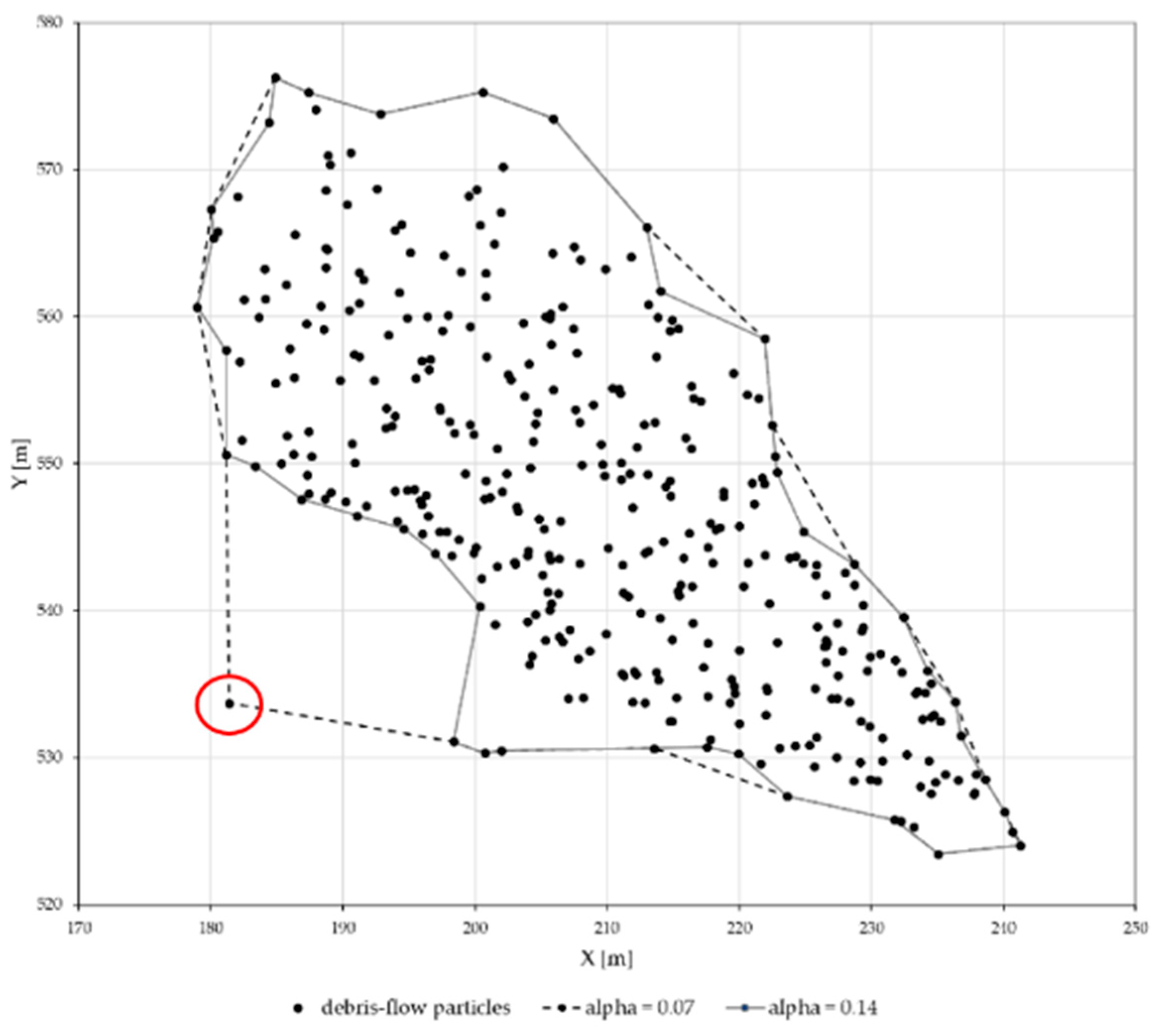
- The boundary polygon generated from the current α value encompasses all the other locations of debris-flow particles. However, the exclusion of the debris-flow particles considered as outliers is acceptable. To determine whether a point location is considered as an outlier, the average space between the debris-flow particles is used. If a location of point A is an outlier, then the average distance from the point A to other points is 1.5 times greater than the average distance between the other points beside the point A, as shown in Figure A1.
Figure A1.
The α-shape with alpha = 0.07 includes an outlier point, while alpha = 0.14 does not include an outlier point. The debris-flow particle, which is considered as outliers, is indicated by a red circle.
Figure A1.
The α-shape with alpha = 0.07 includes an outlier point, while alpha = 0.14 does not include an outlier point. The debris-flow particle, which is considered as outliers, is indicated by a red circle.

- The number of boundary polygons generated from the boundary points by the current α value does not exceed one.
References
- Jakob, M.; Hungr, O. Debris-Flow Hazards and Related Phenomena; Springer: Berlin, Germany, 2005. [Google Scholar]
- Crozier, M.J. Deciphering the effect of climate change on landslide activity: A review. Geomorphology 2010, 124, 260–267. [Google Scholar] [CrossRef]
- Lien, P. Design of Silt Dams for Controlling Stony Debris Flow. Int. J. Sediment Res. 2003, 18, 74–87. [Google Scholar]
- Lucas-Borja, M.E.; Piton, G.; Nichols, M.; Castillo, C.; Yang, Y.; Zema, D. The use of check dams for soil restoration at watershed level: A century of history and perspectives. Sci. Total Environ. 2019, 92, 37–38. [Google Scholar] [CrossRef] [Green Version]
- Rossi, G.; Armanini, A. Impact force of a surge of water and sediments mixtures against slit check dams. Sci. Total Environ. 2019, 683, 351–359. [Google Scholar] [CrossRef]
- McDougall, S. 2014 Canadian Geotechnical Colloquium: Landslide runout analysis—Current practice and challenges. Can. Geotech. J. 2016, 54, 605–620. [Google Scholar] [CrossRef] [Green Version]
- Rickenmann, D. Empirical relationships for debris flows. Nat. Hazards 1999, 19, 47–77. [Google Scholar] [CrossRef]
- Marchi, L.; D’Agostino, V. Estimation of debris-flow magnitude in the Eastern Italian Alps. Earth Surf. Process. Landf. 2004, 29, 207–220. [Google Scholar] [CrossRef]
- Pastor, M.; Blanc, T.; Manzanal, D.; Drempetic, V.; Pastor, M.J.; Sanchez, M.; Crosta, G.; Imposimato, S.; Roddeman, D. Landslide Runout: Review of Analytical/Empirical Models for Subaerial Slides, Submarine Slides and Snow Avalanche. Numerical Modelling. Software Tools, Material Models, Validation and Benchmarking for Selected Case Studies. Available online: https://www.ngi.no/download/file/5981 (accessed on 5 January 2019).
- Osti, R.; Egashira, S. Methods to improve the mitigative effectiveness of a series of check dams against debris flows. Hydrol. Process. 2008, 22, 4986–4996. [Google Scholar] [CrossRef]
- Remaitre, A.; van Asch Heiss, T.W.J.; Malet, G.; Maquaire, O.I. Influence of check dams on debris flow run-out intensity. Nat. Hazards Earth Syst. Sci. 2008, 8, 1403–1416. [Google Scholar] [CrossRef]
- Gregoretti, C.; Stancanelli, M.L.; Bernard, M.; Boreggio, M.; Degetto, M.; Lanzoni, S. Relevance of erosion processes when modelling in-channel gravel debris flows for efficient hazard assessment. J. Hydrol. 2019, 569, 575–591. [Google Scholar] [CrossRef]
- Bernard, M.; Boreggio, M.; Degetto, M.; Gregoretti, C. Model-based approach for design and performance evaluation of works controlling stony debris flows with an application to a case study at Rovina di Cancia (Venetian Dolomites, Northeast Italy). Sci. Total Environ. 2019, 688, 1373–1388. [Google Scholar] [CrossRef] [PubMed]
- Cucchiaro, S.; Cavalli, M.; Vericat, D.; Crema, S.; Llena, M.; Beinat, A.; Marchic, L.; Cazorzi, F. Geomorphic effectiveness of check dams in a debris-flow catchment using multi-temporal topographic surveys. Catena 2019, 174, 73–83. [Google Scholar] [CrossRef]
- McDougall, S. A New Continuum Dynamic Model for the Analysis of Extremely Rapid Landslide Motion across Complex 3D Terrain. Ph.D. Thesis, University of British Columbia, Vancouver, BC, Canada, 2006. [Google Scholar] [CrossRef]
- Lee, D.H.; Lee, S.R.; Park, J.Y. Numerical Simulation of Debris Flow Behavior at Mt. Umyeon using the DAN3D Model. J. Korean Soc. Hazard Mitig. 2019, 19, 195–202. [Google Scholar] [CrossRef]
- Aaron, J.; Hungr, O.; Stark, T.D.; Baghdady, A.K. Oso, Washington, Landslide of March 22, 2014: Dynamic Analysis. J. Geotech. Geoenviron. Eng. 2017, 143, 05017005. [Google Scholar] [CrossRef] [Green Version]
- Choi, S.K.; Kwon, T.H.; Lee, S.R.; Park, J.Y. Roles of barrier location for effective debris flow mitigation: Assessment using DAN3D. In Association of Environmental and Engineering Geologists; Special Publication 28; Colorado School of Mines, Arthur Lakes Library: Golden, CO, USA, 2019. [Google Scholar] [CrossRef]
- Cheon, E.; Lee, S.M.; Lee, S.R.; Lee, D.H.; Kim, M.S.; Lim, H.H. A Framework to Compute the Width and Area of Debris-Flow Based on DAN3D. In Proceedings of the 32nd KKHTCNN Symposium on Civil Engineering, Daejeon, Korea, 24–26 October 2019. [Google Scholar]
- Sarir, P.; Shen, S.L.; Wang, Z.F.; Chen, J.; Horpibulsuk, S.; Pham, B.T. Optimum model for bearing capacity of concrete-steel columns with AI technology via incorporating the algorithms of IWO and ABC. Eng. Comput. 2019, 1, 1–11. [Google Scholar] [CrossRef]
- Zhang, N.; Shen, S.L.; Zhou, A.; Xu, Y.S. Investigation on performance of neural networks using quadratic relative error cost function. IEEE Access 2019, 7, 106642–106652. [Google Scholar] [CrossRef]
- Elbaz, K.; Shen, S.L.; Zhou, A.; Yuan, D.J.; Xu, Y.S. Optimization of EPB shield performance with adaptive neuro-fuzzy inference system and genetic algorithm. Appl. Sci. 2019, 9, 780. [Google Scholar] [CrossRef] [Green Version]
- Lyu, H.M.; Shen, S.L.; Zhou, A.; Yang, J. Perspectives for flood risk assessment and management for mega-city metro system. Tunn. Undergr. Space Technol. 2019, 84, 31–44. [Google Scholar] [CrossRef]
- Lyu, H.M.; Shen, S.L.; Zhou, A.N.; Zhou, W.H. Flood risk assessment of metro systems in a subsiding environment using the interval FAHP–FCA approach. Sustain. Cities Soc. 2019, 50, 101682. [Google Scholar] [CrossRef]
- Hungr, O. A model for the runout analysis of rapid flow slides, debris flows, and avalanches. Can. Geotech. J. 1995, 32, 610–623. [Google Scholar] [CrossRef]
- Hungr, O.; McDougall, S. Two numerical models for landslide dynamic analysis. Comput. Geosci. 2009, 35, 978–992. [Google Scholar] [CrossRef]
- Savage, S.B.; Hutter, K. The motion of a finite mass of granular material down a rough incline. J. Fluid Mech. 1989, 199, 177–215. [Google Scholar] [CrossRef]
- Lucy, L.B. A numerical approach to the testing of the fission hypothesis. Astron. J. 1977, 82, 1013–1024. [Google Scholar] [CrossRef]
- Gingold, R.A.; Monaghan, J.J. Smoothed Particle Hydrodynamics: Theory and application to non-spherical stars. Mon. Not. R. Astron. Soc. 1977, 181, 375–389. [Google Scholar] [CrossRef]
- Monaghan, J.J. Smoothed particle hydrodynamics. Annu. Rev. Astron. Astrophys. 1992, 30, 543–574. [Google Scholar] [CrossRef]
- McDougall, S.; Hungr, O. Dynamic modelling of entrainment in rapid landslides. Can. Geotech. J. 2005, 42, 1437–1448. [Google Scholar] [CrossRef]
- Yoon, S.; Lee, S.R.; Park, J.Y.; Seong, J.H.; Lee, D.H. A prediction of entrainment growth rate for debris-flow hazard analysis using multiple regression analysis. J. Korean Soc. Hazard Mitig. 2015, 15, 353–360. [Google Scholar] [CrossRef] [Green Version]
- Lloyd, S. Least squares quantization in PCM. IEEE Trans. Inf. Theory 1982, 28, 129–137. [Google Scholar] [CrossRef]
- Arthur, D.; Vassilvitskii, S. k-means++: The advantages of careful seeding. In Proceedings of the Eighteenth Annual ACM-SIAM Symposium on Discrete Algorithms, New Orleans, LA, USA, 7–9 January 2007; Society for Industrial and Applied Mathematics Philadelphia: Philadelphia, PA, USA, 2007; pp. 1027–1035. [Google Scholar]
- Aurenhammer, F. Voronoi Diagrams—A Survey of a Fundamental Geometric Data Structure. ACM Comput. Surv. 1991, 23, 345–405. [Google Scholar] [CrossRef]
- Weston.pace; Wikipedia. K Means Example. 2007. Available online: https://en.wikipedia.org/wiki/K-means_clustering#/media/File:K_Means_Example_Step_1.svg (accessed on 1 December 2019).
- Ketchen, D.J.; Shook, C.L. The application of cluster analysis in strategic management research: An analysis and critique. Strateg. Manag. J. 1996, 17, 441–458. [Google Scholar] [CrossRef]
- sklearn.cluster.KMeans. Available online: https://scikit-learn.org/stable/modules/generated/sklearn.cluster.KMeans.html (accessed on 2 August 2019).
- Edelsbrunner, H.; Kirkpatrick, D.G.; Seidel, R. On the shape of a set of points in the plane. IEEE Trans. Inf. Theory 1983, 29, 551–559. [Google Scholar] [CrossRef] [Green Version]
- de Berg, M.; van Kreveld, M.; Overmars, M.; Schwarzkopf, O. Computational Geometry: Algorithms and Applications; Springer: Berlin, Germany, 2000; pp. 2–8. [Google Scholar]
- Drawing Boundaries in Python. Available online: http://blog.thehumangeo.com/2014/05/12/drawing-boundaries-in-python/ (accessed on 28 August 2019).
- Shimrat, M. Algorithm 112: Position of point relative to polygon. Commun. ACM 1962, 5, 434. [Google Scholar] [CrossRef]
- Zanchetta, G.; Sulpizio, R.; Pareschi, M.T.; Leoni, F.M.; Santacroce, R. Characteristics of May 5–6, 1998 Volcaniclastic Debris-flows in the Sarno Area of Campania, Southern Italy: Relationships to Structural Damage and Hazard Zonation. J. Volcanol. Geotherm. Res. 2004, 133, 377–393. [Google Scholar] [CrossRef]
- Hu, K.H.; Cui, P.; Zhang, J.Q. Characteristics of Damage to Buildings by Debris Flows on 7 August 2010 in Zhouqu, Western China. Nat. Hazards Earth Syst. Sci. 2012, 12, 2209–2217. [Google Scholar] [CrossRef]
- Kang, H.S.; Kim, Y.T. Physical vulnerability function of buildings impacted by debris flow. J. Korean Soc. Hazard Mitig. 2014, 14, 133–143. [Google Scholar] [CrossRef] [Green Version]
- Kwan, J.S.H. Supplementary technical guidance on design of rigid debris-resisting barriers. In Geotechnical Engineering Office HKSAR; GEO Report No. 270; Geotechnical Engineering Office: Kowloon, Hong Kong, 2012. [Google Scholar]
- Hübl, J.; Nagl, G.; Suda, J.; Rudolf-Miklau, F. Standardized stress model for design of torrential barriers under impact of debris flow (according to Austrian standard regulation 24801). Int. J. Erosion Control Eng. 2017, 10, 47–55. [Google Scholar] [CrossRef] [Green Version]
- Yune, C.Y.; Chae, Y.K.; Paik, J.; Kim, G.; Lee, S.W.; Seo, H.S. Debris flow in metropolitan area—2011 Seoul debris flow. J. Mt. Sci. 2013, 10, 199–206. [Google Scholar] [CrossRef]
- Korean Society of Civil Engineers. Research Contract Report: Addition and Complement Causes Survey and Restoration Work of Mt. Umyeon Landslide. Available online: http://www.j-kosham.or.kr/journal/Table.php?xn=kosham-19-3-195.xml&id=&mode=export (accessed on 6 January 2020).
Figure 1.
The continuous landslide mass in the orthogonal grid is discretized into debris-flow particles (represented as dots), which are evenly placed within the grid.
Figure 1.
The continuous landslide mass in the orthogonal grid is discretized into debris-flow particles (represented as dots), which are evenly placed within the grid.

Figure 2.
The overall flowchart of the developed framework to compute the parameters of debris-flow.
Figure 2.
The overall flowchart of the developed framework to compute the parameters of debris-flow.

Figure 3.
A simple demonstration of the k-means clustering algorithm [36] with the following procedures: (a) initialization, (b) partition, (c) new centroid, and (d) stopping criterion.
Figure 3.
A simple demonstration of the k-means clustering algorithm [36] with the following procedures: (a) initialization, (b) partition, (c) new centroid, and (d) stopping criterion.

Figure 4.
Comparison of the Convex Hull (dotted line) and the α-shape with alpha = 0.07 (solid line) over a selection of debris-flow particles.
Figure 4.
Comparison of the Convex Hull (dotted line) and the α-shape with alpha = 0.07 (solid line) over a selection of debris-flow particles.

Figure 5.
The criteria to determine the merging of two debris-flow clusters A and B by comparing the travel directions and assessing the number of debris-flow particles in the overlapping region.
Figure 5.
The criteria to determine the merging of two debris-flow clusters A and B by comparing the travel directions and assessing the number of debris-flow particles in the overlapping region.

Figure 6.
The criteria indicating splitting of a debris-flow cluster: (a) the centroid of the debris-flow cluster is outside the boundary of the debris-flow cluster, and (b) plotting the frequency distribution of the travel direction of debris-flow particles shows two distinct peaks in the first panel.

Figure 7.
A simple example showing the application of the even–odd rule algorithm to determine that the white cross and the black cross are outside and inside the polygon region, respectively.
Figure 7.
A simple example showing the application of the even–odd rule algorithm to determine that the white cross and the black cross are outside and inside the polygon region, respectively.

Figure 8.
The definition of the width of a debris-flow cluster [19].
Figure 8.
The definition of the width of a debris-flow cluster [19].

Figure 9.
The distribution of pressure applied to the barrier surface: (a) dynamic debris-flow cluster (v ≠ 0), and (b) static debris-flow cluster (v = 0).
Figure 9.
The distribution of pressure applied to the barrier surface: (a) dynamic debris-flow cluster (v ≠ 0), and (b) static debris-flow cluster (v = 0).

Figure 10.
The combination of pressures applied to the barrier surface from the dynamic and static debris-flow clusters. The pressure distributions are separated for clarity. The point O refers to the pivot point at which the moment applied to the barrier by the debris-flow clusters is computed.
Figure 10.
The combination of pressures applied to the barrier surface from the dynamic and static debris-flow clusters. The pressure distributions are separated for clarity. The point O refers to the pivot point at which the moment applied to the barrier by the debris-flow clusters is computed.

Figure 11.
The flowpaths of the debris-flow that affected the Raemian and Sindonga regions are marked with yellow lines [16].
Figure 11.
The flowpaths of the debris-flow that affected the Raemian and Sindonga regions are marked with yellow lines [16].

Figure 12.
The Surfer grid files used for DAN3D that provide the following information: (a) path topography, (b) initial source, and (c) erosion map for the Raemian region [16].
Figure 12.
The Surfer grid files used for DAN3D that provide the following information: (a) path topography, (b) initial source, and (c) erosion map for the Raemian region [16].

Figure 13.
Comparison of results from (a) the initial landslide source [16] and (b) the k-means clustering algorithm and the Elbow method against the initial landslide region. The different debris-flow clusters are represented in different colors. The red dots indicate the centroid of each cluster.
Figure 13.
Comparison of results from (a) the initial landslide source [16] and (b) the k-means clustering algorithm and the Elbow method against the initial landslide region. The different debris-flow clusters are represented in different colors. The red dots indicate the centroid of each cluster.

Figure 14.
The hazard assessment map generated from the developed framework showing the different flowpaths that originated from the four sources indicated by circled numbers. The rectangles show the locations of proposed potential closed-type barriers for mitigation against the debris-flow.
Figure 14.
The hazard assessment map generated from the developed framework showing the different flowpaths that originated from the four sources indicated by circled numbers. The rectangles show the locations of proposed potential closed-type barriers for mitigation against the debris-flow.

Figure 15.
The hazard assessment map generated from the developed framework showing the width (unit: m) of the debris-flow cluster for (a) flowpath A, (b) flowpath B, and (c) flowpath C. The flowpaths are plotted separately for clarity.
Figure 15.
The hazard assessment map generated from the developed framework showing the width (unit: m) of the debris-flow cluster for (a) flowpath A, (b) flowpath B, and (c) flowpath C. The flowpaths are plotted separately for clarity.

Figure 16.
The hazard assessment map generated from the developed framework showing the volume (unit: m3) of debris-flow clusters for (a) flowpath A, (b) flowpath B, and (c) flowpath C. The flowpaths are plotted separately for clarity.
Figure 16.
The hazard assessment map generated from the developed framework showing the volume (unit: m3) of debris-flow clusters for (a) flowpath A, (b) flowpath B, and (c) flowpath C. The flowpaths are plotted separately for clarity.

Figure 17.
The hazard assessment map generated from the developed framework showing the impact pressure (unit: kPa) of the debris-flow cluster for (a) flowpath A, (b) flowpath B, and (c) flowpath C. The flowpaths are plotted separately for clarity.
Figure 17.
The hazard assessment map generated from the developed framework showing the impact pressure (unit: kPa) of the debris-flow cluster for (a) flowpath A, (b) flowpath B, and (c) flowpath C. The flowpaths are plotted separately for clarity.


Table 1.
The input values used in DAN3D for simulating debris-flow at Umyeon mountain [16].
Table 1.
The input values used in DAN3D for simulating debris-flow at Umyeon mountain [16].
| Parameter | Properties (Unit) | Value |
|---|---|---|
| Soil | Unit Weight (kN/m3) | 18.5 |
| Internal Friction Angle (°) | 22.4 | |
| Maximum Erosion Depth (m) | 4 | |
| Density (kg/m3) | 2000 | |
| Bingham Model Basal Rheology | Volumetric Concentration of Sediments | 0.375 |
| Yield stress (Pa) | 7.29 | |
| Viscosity (Pa∙s) | 0.05 | |
| Entrainment | Erosion Growth Rate (%/m) | 0.00421 |
Table 2.
The impact parameters from the collisions between the debris-flow and barrier.
| Barrier | Impact Parameter (Unit) | Value |
|---|---|---|
| X | Location X-coordinate (m) | 405.0 |
| Location Y-coordinate (m) | 170.0 | |
| Width (m) | 43.8 | |
| Volume (m3) | 2388.0 | |
| Force (MN) | 47.4 | |
| Moment (MNm) | 21.4 | |
| Y | Location X-coordinate (m) | 375.0 |
| Location Y-coordinate (m) | 392.0 | |
| Width (m) | 75.4 | |
| Volume (m3) | 1345.0 | |
| Force (MN) | 111.5 | |
| Moment (MNm) | 34.9 |
© 2020 by the authors. Licensee MDPI, Basel, Switzerland. This article is an open access article distributed under the terms and conditions of the Creative Commons Attribution (CC BY) license (http://creativecommons.org/licenses/by/4.0/).
Share and Cite
MDPI and ACS Style
Cheon, E.; Lee, S.-R.; Lee, D.-H. Hazard Assessment Based on the Combination of DAN3D and Machine Learning Method for Planning Closed-Type Barriers against Debris-Flow. Water 2020, 12, 170. https://doi.org/10.3390/w12010170
AMA Style
Cheon E, Lee S-R, Lee D-H. Hazard Assessment Based on the Combination of DAN3D and Machine Learning Method for Planning Closed-Type Barriers against Debris-Flow. Water. 2020; 12(1):170. https://doi.org/10.3390/w12010170
Chicago/Turabian StyleCheon, Enok, Seung-Rae Lee, and Deuk-Hwan Lee. 2020. "Hazard Assessment Based on the Combination of DAN3D and Machine Learning Method for Planning Closed-Type Barriers against Debris-Flow" Water 12, no. 1: 170. https://doi.org/10.3390/w12010170
Note that from the first issue of 2016, this journal uses article numbers instead of page numbers. See further details here.