Conditions of Hydraulic Heterogeneity under Which Bayesian Estimation is More Reliable
by
Hao-Qing Yang
1,2,3, 
Xiangyu Chen
1,2,3,
Lulu Zhang
1,2,3,*,
Jie Zhang
4,
Xiao Wei
5 and
Chong Tang
5 1
State Key Laboratory of Ocean Engineering, Shanghai Jiao Tong University, Shanghai 200240, China
2
Collaborative Innovation Center for Advanced Ship and Deep-Sea Exploration (CISSE), Shanghai 200240, China
3
Department of Civil Engineering, Shanghai Jiao Tong University, Shanghai 200240, China
4
Key Laboratory of Geotechnical and Underground Engineering of Ministry of Education and Department of Geotechnical Engineering, Tongji University, Shanghai 200092, China
5
Department of Civil and Environmental Engineering, National University of Singapore, Singapore 119077, Singapore
*
Author to whom correspondence should be addressed.
Water 2020, 12(1), 160; https://doi.org/10.3390/w12010160
Submission received: 23 November 2019
/
Revised: 1 January 2020
/
Accepted: 3 January 2020
/
Published: 4 January 2020
(This article belongs to the Section Hydraulics and Hydrodynamics)
Abstract
:Natural heterogeneity of soil hydraulic properties is significant for the design and construction of geotechnical structures, and should be adequately characterized. Accurate measurements of hydraulic properties remain a difficult job and do not always work well for further design and analysis. Field hydraulic monitoring data reflects the overall slope performance and provide a more representative estimation of in-situ soil hydraulic properties for back analysis. The objective of this study is to explore the conditions under which monitoring data can provide reliable estimates of hydraulic parameters. Different distributions of soil heterogeneity generate a total number of 500 sets of synesthetic monitoring data. Bayesian inversion with the integration of Karhunen-Loève (K-L) and polynomial chaos expansion (PCE) is chosen to estimate the spatially varied saturated coefficient of permeability ks. The results show that the method is accurate and reliable, with less than 3% percentage error and 0.08 coefficient of variation (COV) around the monitoring points. There are two characteristics of the best-estimated fields. First, the ranges of ks for best-estimated fields are much narrower than the worst estimated fields. Second, when the larger ks values are distributed in the unsaturated zone of slope crest, it will lead to the best estimation. It is suggested that monitoring data can provide a reliable estimation of heterogeneous ks when the ratio of ground surface flux to ks in the unsaturated zone of slope crest is less than 1/150. Small values of ks in the slope crest result in the response of pressure head far from the responses of homogenous ks in the unsaturated zone. This complex response of the pressure head further causes the ill identification of ks by Bayesian estimation.
1. Introduction
Water-induced slope failure is a common geological disaster threatening infrastructures and lives. Severe rainfall events, intense storms, changes in groundwater level, snowmelt and roaring waves substantially affect the mechanical and infiltration processes and consequently lead to the instability of slopes [1,2,3,4]. Thus, proper characterization of hydraulic properties in slopes can better assess the stability and mitigate the water-induced slope failures.
The hydraulic properties of the soil, which are the key parameters to affect the infiltration process, fluctuate in response to the infiltration and atmospheric condition. Despite the sophisticated development of laboratory and in-situ tests, it has been widely observed that an accurate measurement of hydraulic properties remains a difficult job. The main disadvantages of laboratory and in-situ analysis of soil hydraulic properties are summarized below [5,6,7]. First, permeability is sensitive to the sampling method and experimental condition, due to the redistribution of pore water and air. Second, the measurement of soil hydraulic properties suffers from severe variability. For example, the coefficient of variation of the saturated coefficient of permeability ks can be ranged from 50% to 450% according to Carsel and Parrish (1988) [8]. Third, to ensure acceptable reliability, a large number of tests are often required in the field, adopting complicated sampling and testing techniques that consume a lot of time and budget. Therefore, the inferred hydraulic properties from the laboratory or in-situ tests do not always work well for further design and analysis.
To overcome the limitations of in-situ and laboratory testing, many researchers adopted inverse method to back analyze the soil hydraulic properties for the interests of geotechnical engineering based on model responses (recorded as monitoring data) [9,10,11,12]. In recent years, Bayesian approaches have been utilized to estimate soil hydraulic properties with monitoring data. Zhang et al. (2014) [10] calibrated a slope-stability model using time-varying response data and to justify appropriate monitoring duration and data recording interval for field monitoring programs. Vardon et al. (2016) [13] presented an inverse analysis with the ensemble Kalman filter method to reduce the spatial uncertainty of hydraulic conductivity by utilizing pore pressure measurements. Gomes et al. (2017) [14] investigated the uncertainty of the bedrock depth and soil hydraulic parameters on the stability of an unsaturated slope in Rio de Janeiro, Brazil. Li et al. (2018) [15] updated the reliability of hydraulic head monitoring data under a Bayesian framework. Yang et al. (2018) [16] proposed an efficient Bayesian method for probabilistic estimation of spatially varied soil properties in a slope. Zheng et al. (2018) [17] employed the Bayesian approach with various types of data to yield accurate predictions of consolidation for a test embankment in New South Wales, Australia. These studies demonstrated that field hydraulic monitoring data reflects the actual overall slope performance and can provide a more representative estimation of in-situ soil hydraulic properties. However, among all these previous studies, limited work is concerned with the soil heterogeneity [13,16].
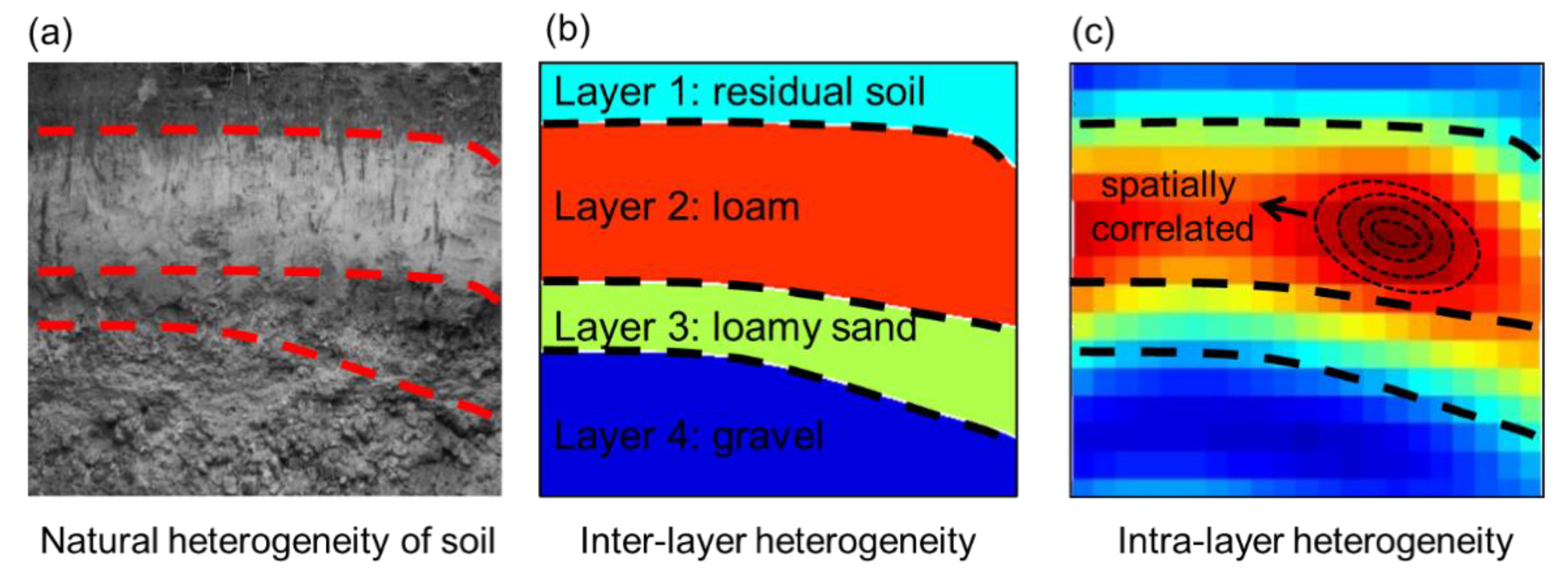
Significant natural heterogeneity is observed in the field for soil hydraulic properties (Figure 1a). The distribution of soil heterogeneity has a significant impact on the safety of geotechnical structures and should be characterized properly [18,19,20,21]. There are two types of spatial heterogeneity, namely, inter-layer and intra-layer heterogeneity.
In general, the entire ground can be divided into strata or layers. Soil parameters can be viewed as statistically homogenous in a given stratum or layer (Figure 1b). However, the soils are heterogeneous in the vertical direction, due to natural pedological processes. In this sense, inter-layer heterogeneity means that different strata or layers have different properties. Field investigations, experimental studies, and numerical simulations have been carried out to study the influence of inter-layer heterogeneity on rainfall infiltration characteristics and slope stability [22,23,24,25]. If the hydraulic properties are heterogeneously distributed, a sudden change in pore pressure and water content will be observed at the interface of the formation—this can affect the advancement of the wetting front. The failure modes and safety factor of the slope also change [26,27].
Intra-layer heterogeneity means that soil properties vary spatially even within a given soil layer. The values of soil properties are different from point to point, but are spatially correlated (Figure 1c). The correlation structure can be used to describe spatial variations of soil properties within the framework of random fields effectively [28]. This inherent heterogeneity is a major source of geotechnical uncertainty and has significant impacts on the reliability of slope stability [29,30,31]. For the rainfall-induced slope failures, the intra-layer heterogeneity leads to the propagation of the uncertainty of soil hydraulic properties to variation of water pressure and fluctuation of the groundwater table. The factor of safety of slope stability and the probability of slope failure are also influenced.
Up to the present, theoretical studies of the influence of the heterogeneity of hydraulic parameters on the field responses of slopes (i.e., forward problems) are quite developed [19,20]. However, for the inverse problem, the related studies are still very limited [13,16]. Previous studies only considered one specific distribution of material heterogeneity to verify and illustrate the proposed various methods [32,33,34,35,36]. In reality, the natural heterogeneity of soils is extremely diverse. The performance of inverse analysis methods for different ground situations has not been fully investigated. The conditions of soil heterogeneity under which the monitoring data can provide a more reliable estimation of soil hydraulic properties remains an open question.
In previous studies, our research team has demonstrated that the Bayesian method can be used to estimate the heterogeneity of hydraulic properties in unsaturated soil slopes [16]. The combination of Karhunen-Loève (K-L) expansion and the polynomial chaos expansion (PCE) can successfully reduce the computation load with acceptable accuracy. Suggestions for planning slope monitoring schemes were provided [36].
The objective of this study is to investigate the conditions under which monitoring data can provide a more reliable estimation of heterogeneous hydraulic properties. The performance of Bayesian estimation for different realizations of the saturated coefficient of permeability ks is assessed based on the criteria of mutual information (I), and the root mean square error (RMSE). The effect of heterogeneity is studied with sensitivity analysis. The relationship between estimated error and monitoring response is measured by the metric similarity. Instead of introducing a new inverse method, the methodology in our previous study [16] is adopted, due to its high computational efficiency. Other inverse methods can also be used.
2. Bayesian Estimation of Heterogeneity with Polynomial Chaos Expansion and Karhunen-Loève Expansion
Bayesian estimation with integration of the polynomial chaos expansion (PCE) surrogate model and the Karhunen-Loève (K-L) expansion is emerged to estimate material heterogeneity in recent years [32,33,34,35,36]. To solve high-dimensional inverse problems, K-L expansion is adopted to transform the inverse problem to inference on a truncated sequence of weights of the K-L expansion modes. To accelerate the computational efficiency in Bayesian inference, PCE is constructed as a meta-model to surrogate the original model. As a result, the calculation of system responses using a simple equation consisting of polynomials is allowed. The purpose of this study focuses on the effect of soil heterogeneity instead of the methodology. Therefore, a brief introduction of the method [16] is described here. Detailed descriptions of the method can be found in Yang et al. (2018) [16].
The computational cost of the numerical prediction would be extremely large, due to the increase of nonlinearity of the boundary value problem [37,38,39]. Therefore, the first step is to establish the surrogate model for responses of the numerical model and random variables in K-L expansion by polynomial chaos expansion (PCE) [40,41]:
where j denotes the index of polynomials; m denotes the total number of polynomials; cj is coefficient; θ is the random variables in K-L expansion; ψj(θ) are polynomials; P(θ) is the response of the numerical model.
Second, the random variables θ are estimated by Markov chain Monte Carlo (MCMC) in conjunction with corresponding monitoring data in a Bayesian framework. The posterior probability density function of θ is expressed as follows [42]:
where const is a normalizing constant; f(θ) is the prior distribution of θ; is the variance of the residual error; is a vector of monitoring data; is the monitoring data from the tth measurement point and T is the total number of the measurement points.
Finally, the estimated random variables are transferred to the estimated field by K-L expansion. the spatially varied soil properties U(x) is expressed as:
where x denotes a vector of spatial coordinates; μ(x) is the mean of U(x); θi is the ith uncorrelated Gaussian random variable; n is the truncated level; λi and φi(x) are the ith eigenvalues and eigenvectors of the covariance function, respectively. In practice, covariance function is estimated from sample data or fitted to parametric variogram models.
3. Modeling of Unsaturated Infiltration in a Soil Slope with Spatially Heterogeneous ks Field
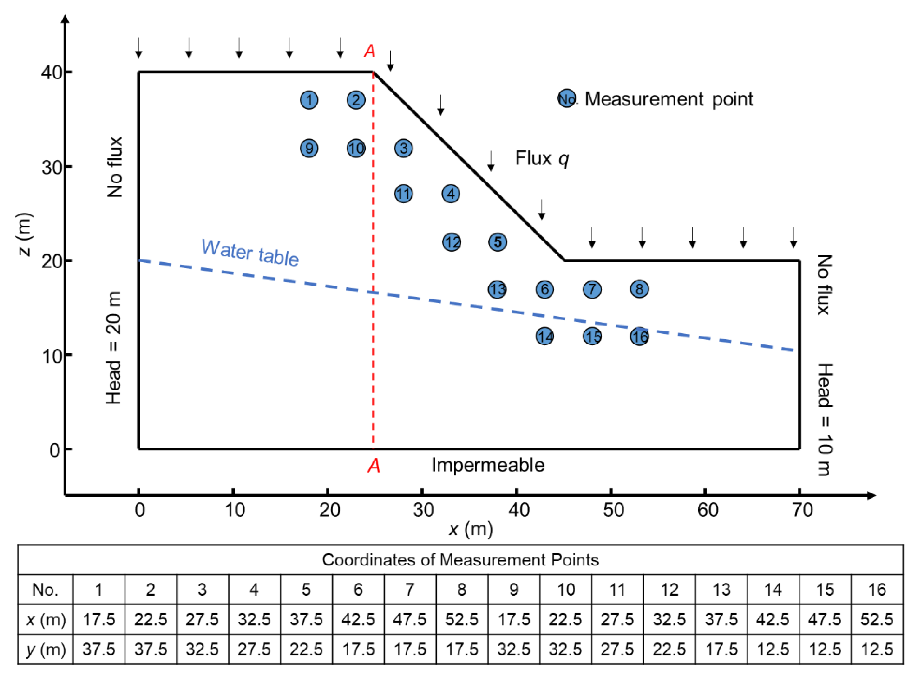
A typical unsaturated soil slope subject to rainfall infiltration with heterogeneous ks field is modeled. The slope angle is 45°, and the slope is 20 m high (Figure 2). The mean value and standard deviation of ks are 2 × 10⁻⁵ m/s and 1.6 × 10⁻⁵ m/s, respectively. The horizontal correlation length lx and vertical correlation length lz are assumed to be 50 m and 10 m, respectively. Six K-L terms are sufficient to preserve 95% of the total field variance. Therefore, the truncation level of the K-L expansion is 6.
The numerical model of unsaturated infiltration in the heterogeneous soil slope is established to model the infiltration and pore pressure responses. According to Darcy’s law and the conservation law of water mass in soil pores, the steady-state flow in an unsaturated soil slope can be described as:
where H is the total hydraulic head, which is the sum of elevation head z and pore-water pressure head h; k is the unsaturated coefficient of permeability. Here, the permeability of the soil slope is assumed to be isotropic with the unsaturated coefficient of permeability of x-direction and z-direction are the same.
Laboratory studies have shown that there is a relationship between water content and soil suction (negative pressure) for the unsaturated soil defined as soil-water characteristic curve (SWCC). Direct measurements of the unsaturated coefficient of permeability in the laboratory can be time-consuming, especially for low water content conditions. Indirect measurements of permeability are commonly performed by establishing permeability functions (PF) through SWCC. Several models of hydraulic properties are proposed for unsaturated soil [43,44,45,46]. Concerning geotechnical applications, the model proposed by Fredlund et al. (2012) [47] is adopted. An exponential PF is used to define the unsaturated coefficient of permeability function [48]:
where ks is the saturated coefficient of permeability, θw is the volumetric water content, θs is the saturated water content, and b is a constant depending on the soil type. The SWCC is described as [49]:
where ua and uw represent the pore-air pressure and the pore-water pressure, respectively; af, nf and mf are fitting parameters. In this study, we assume that the saturated water content θs is 0.4, b is equal to 3 and the SWCC parameters for af, nf and mf are 5, 2 and 1, respectively.
The numerical model of an unsaturated soil slope under the steady-state rainfall infiltration is established using a Multiphysics PDE (partial differential equation) solver COMSOL. The initial pore-water pressure distribution is hydrostatic with the initial groundwater level, as shown in Figure 2. The rain flux, q = 2 × 10⁻⁷ m/s, is applied along the slope surface. Along the left and right boundaries beneath the groundwater table, the hydraulic heads are constant. A zero-flux boundary is applied along the left and right boundaries above the groundwater table. The bottom boundary is impermeable.
4. Artificial Monitoring Scheme for Inverse Estimation
The rainfall-induced slope failures are typically shallow above the groundwater table [50,51]. It is mainly due to a loss in shear strength when soil suctions (i.e., negative pressure head) is decreased or dissipated [47,52]. In engineering practice, shallow piezometers are generally installed to monitor the pressure heads in the slope. For example, the automatic recording piezometers are installed from 1.00 m to 16.6 m below ground level in a natural terrain above the North Lantau Expressway in Hong Kong reported from Evans and Lam (2003) [53]. It is, therefore, reasonable to place measurement points in shallow depth for property estimation. In this study, a monitoring scheme of eight boreholes with a horizontal spacing of 5 m is established within the shallow depths of the slope (Figure 2). Two piezometers are installed in each borehole. The shallower piezometer is 2.5 m below the ground, and the deeper one is 7.5 m depth. The corresponding pore pressure heads calculated by the numerical model, which are corrupted with 2% noises are regarded as synthetic monitoring data.
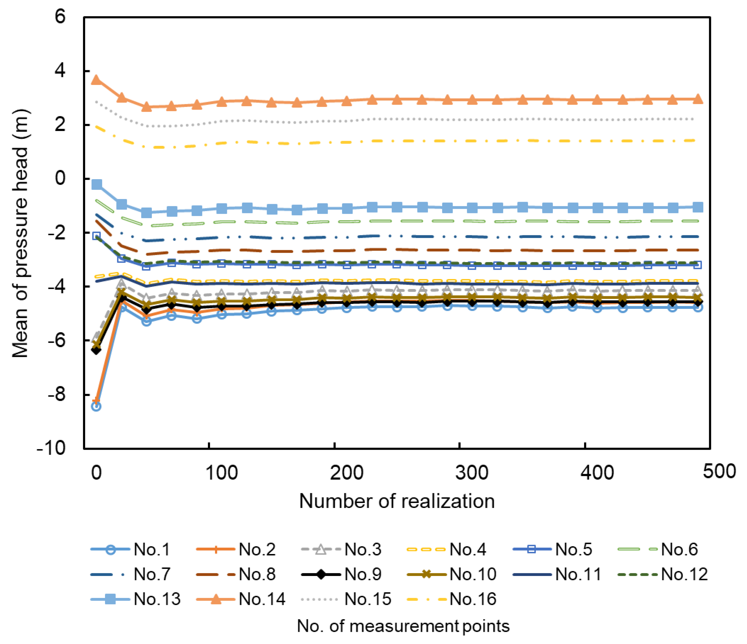
To determine the characteristics of heterogeneity for a robust back estimation, 500 random realizations of the ks field are generated. Figure 3 presents the mean value of the pressure head at 16 different measurement points with the increasing number of realizations. As shown in the graph, there is a small fluctuation of pressure head when the number of realizations reaches 500. This result shows that 500 realizations are enough for covering the uncertainties of pressure head responses for heterogeneity estimation.
5. Performance Evaluation of Inverse Estimation
5.1. Quantification of Parametric Uncertainty Reduction
The outcomes of the Bayesian inference are the posterior distributions of basic random variables θ. To quantify the effects of inverse estimation, the mutual information (I) based on Shannon entropy [54] is used. The Shannon entropy for a continuous random variable with probability density function f(θ) within [a, b] is called differential entropy:
For continuous variables, the differential entropy itself cannot signify the effects of inverse estimation. The mutual information I is proposed to quantify the amount of information obtained through the observed data :
where H(θ) is the differential entropy of prior probability density distribution of θ, which is regarded as a measure of uncertainty about θ; H(θ|) denotes the differential entropy of the posterior probability density distribution of θ, which means the amount of uncertainty remaining about θ after the data is observed.
5.2. Quantification of Estimated Field
The estimated fields can be simulated via the K-L expansion with the statistics of posterior distributions. In this study, the maximum a posteriori density (MAP) value denoting the best solution from Bayesian inverse estimation is utilized to represent the optimal estimated field. The root mean square error (RMSE) is calculated to evaluate the difference between the true field and the best-estimated field:
where is the optimal estimated value with MAP at coordinate xi = (xj, zj) corresponding to ks(xj); L is the total number of the discrete coordinates of the spatial varied field. RMSE can be regarded as an integrated index to rank the results of the estimated fields.
6. Results and Discussion
6.1. Performance Evaluations Based on Synthetic Monitoring Data
Figure 4 shows the mean I value of random variables θ1–θ6 of 500 sets of synthetic monitoring data. The mean I value of each random variable is around two nats. It indicates that a significant difference exists between prior and posterior distributions of random variables. All the random variables are well identified, and the uncertainties are significantly reduced after inverse estimation. The I value of θ1, θ4, and θ5 are 2.48, 2.30, and 2.14 nat, respectively, which are much larger than θ2 and θ3. This means θ1, θ4 and θ5 are better estimated than θ2 and θ3. This finding is consistent with the sensitivity analysis results, according to Yang et al. (2018).
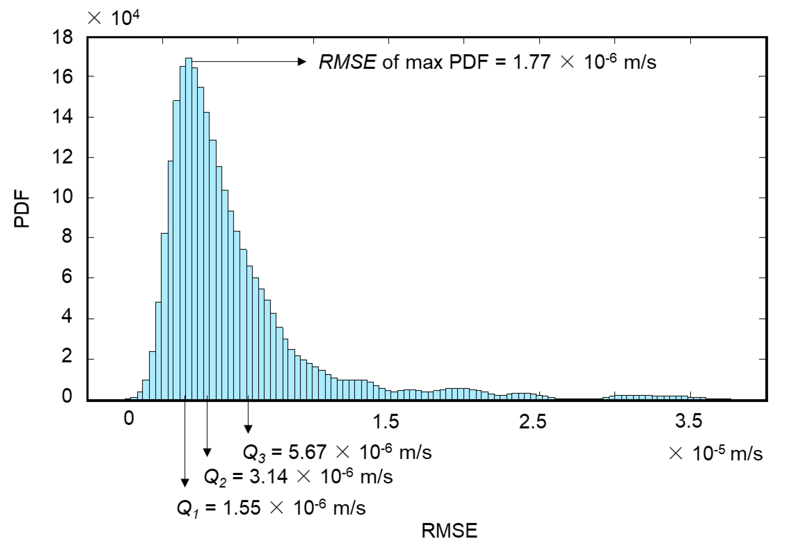
Figure 5 displays the probability density function of the RMSE based on 500 estimated fields. The RMSE corresponding to the maximum probability density is 1.77 × 10⁻⁶ m/s. The median (Q2) value is 3.14 × 10⁻⁶ m/s, which can represent the typical error of the estimated fields. The interquartile range (IQR, upper quartile, Q3—lower quartile, Q1) is 4.12 × 10⁻⁶ m/s, which is narrow compared to the full range. It indicates the major RMSE values are allocated within a narrow range of RMSE. The error of the estimated fields is centralized in a narrow range from 1.55 × 10⁻⁶ m/s to 5.67 × 10⁻⁶ m/s.
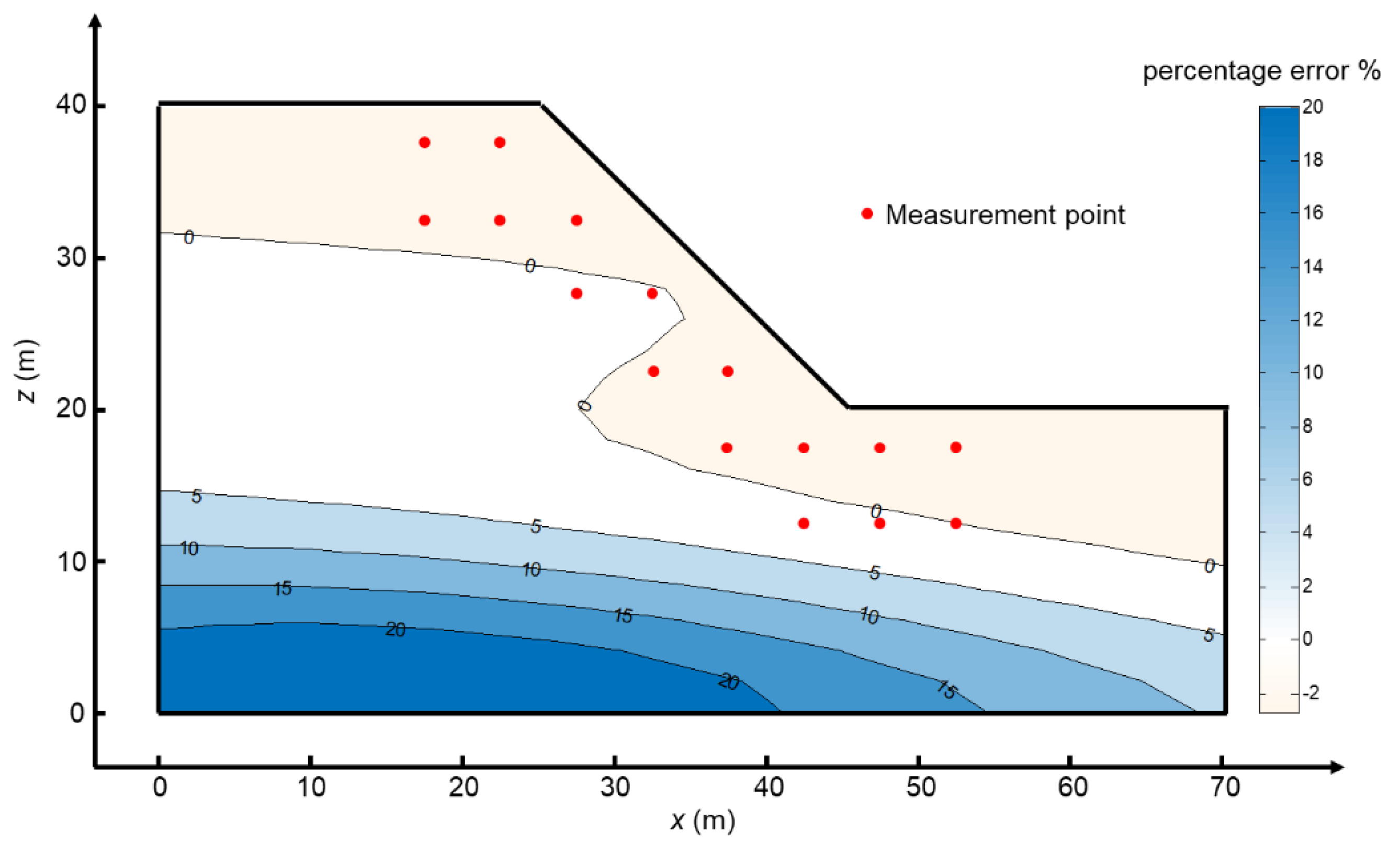
Figure 6 shows the contour map of the mean percentage error with 500 random fields. It is the average value of the percentage error of 500 random fields with the simulation of MAP value in posterior distributions. The percentage error around the measurement points is less than 3%, whereas, the maximum is 20% near the bottom boundary. The significant difference between the real and estimated field occurs at locations that are far from the measurement points.
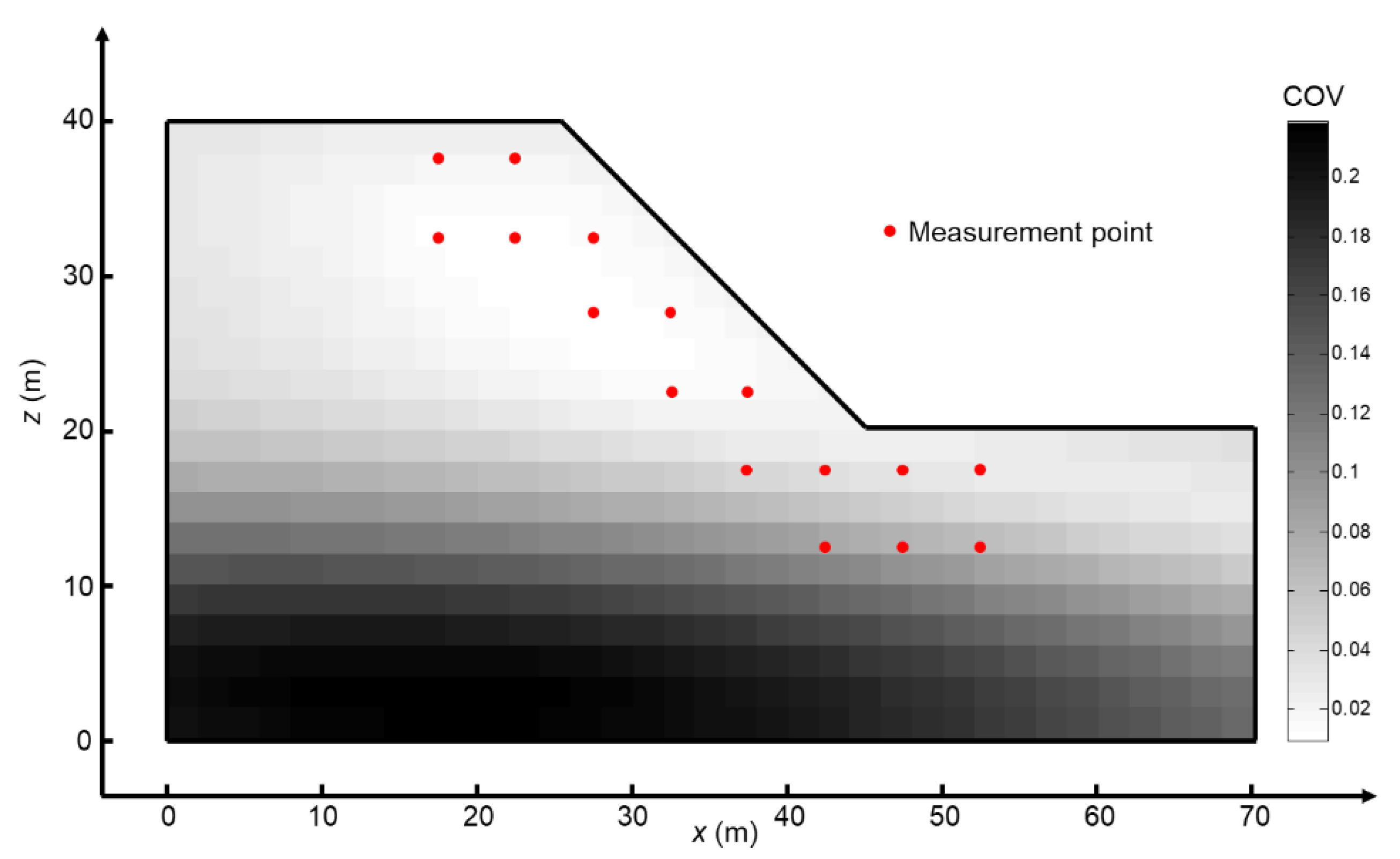
Figure 7 shows the mean value of Coefficient of variation (COV) with 500 random fields. The COV in each field is defined as the ratio of the standard deviation to the mean value based on the last 20% samples of the posterior distribution. It can be observed that the COV around the measurement points is very small, which is less than 0.08. This means that the uncertainty of estimation around measurement points is low. The uncertainty of estimation is significant near the bottom boundary, and the COV is approximate to 0.22. The above results show that the measurement points can reduce the error and uncertainty of the inverse estimation of heterogeneity.
6.2. Analysis of the Effect of Heterogeneity with Extreme RMSE Values
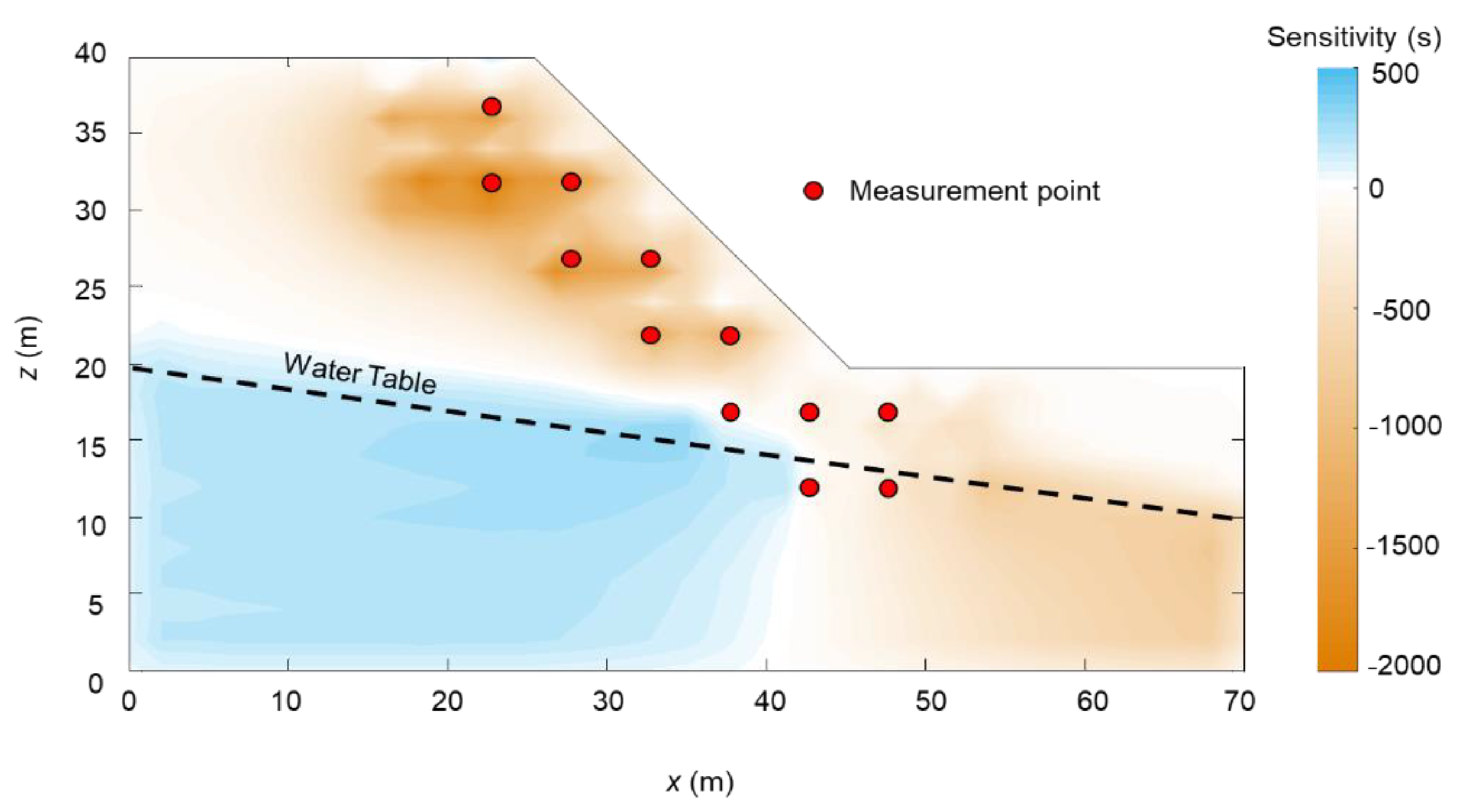
Sensitivity analysis of the pressure head is conducted at measurement points with respect to ks. Taking the partial derivative of the output pressure head with respect to the input parameter ks, small perturbations of ks with 2% are exanimated at each location in the field. The average sensitivity of pressure head at measurement points is shown in Figure 8. The sensitivity away from the slope and below the water table is positive, indicating the average pressure head of sixteen measurement points will increase along with the increasing ks and vice versa. Opposite effects occur in the crest, slope part, and toe. Sensitivity in the crest is extremely large. It means that the ks in the crest zone has a noteworthy influence on the average pressure head responses. The change of ks in the crest can cause significant uncertainty in the average pressure head responses. Therefore, the slope can be divided into two parts bounded by the water table. The relationship between the characteristics of distributed ks on both sides and the estimated effects are worth studying. Moreover, the responses of pressure head in the crest, according to the ks, should be the focus of attention.
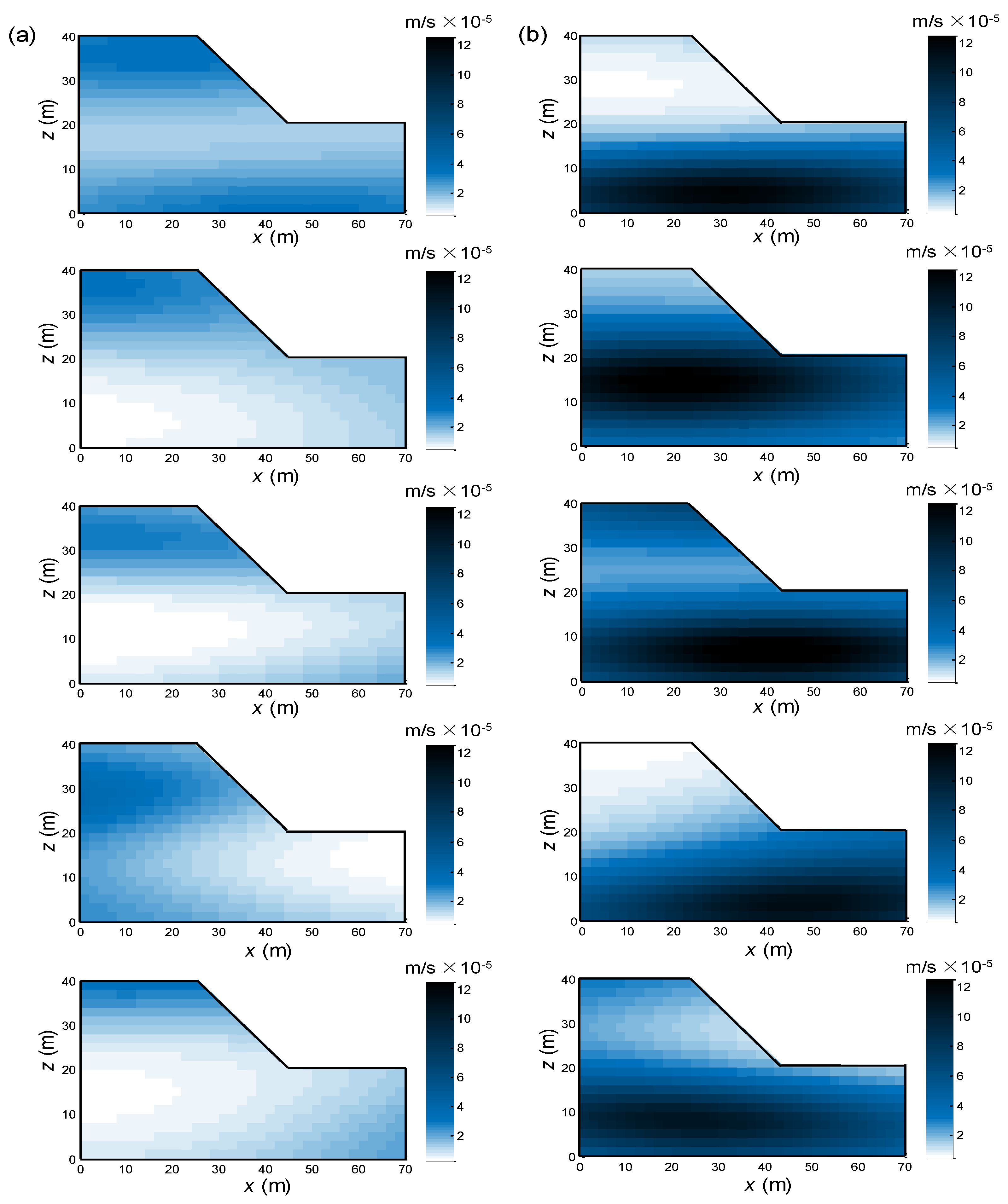
To analyze the characteristics of the heterogeneous fields, the 500 realizations of heterogeneous fields are ranked by the RMSE values of estimation. Figure 9a shows the first five fields, which are best-estimated. The mean RMSE of these fields is 2.75 × 10⁻⁷ m/s. Figure 9b shows the first five worst-estimated fields. The mean RMSE is 3.21 × 10⁻⁵ m/s. The RMSEs of these ten fields are listed in Table 1. There are nearly two orders of magnitude differences in terms of the RMSEs. The distribution of heterogeneity can significantly influence the effect of inverse estimation. Compared to the first five best and worst real fields, there are two characteristics of the range and the distribution of ks. First, the ks of the best-estimated fields range from 0.35 × 10⁻⁵ m/s to 3.92 × 10⁻⁵ m/s, which is much narrower than the worst estimated fields ranging from 0.55 × 10⁻⁵ m/s to 12.99 × 10⁻⁵ m/s. Second, when the larger ks values (around 3 × 10⁻⁵ m/s) are distributed in the unsaturated zone of slope crest, it will lead to the best estimation. However, the distribution of ks for the worst estimated fields is reversed. For these fields, the crest part of the slope is generally less permeable compared with the main body part of the slope. According to Zhang et al. (2004) [55], the steady-state matric suction in the unsaturated zone can be determined by the ratio of ground surface flux to the saturated coefficient of permeability, q/ks. Therefore, a reliable estimation of the heterogeneous field of ks can be obtained when the q/ks in the slope crest is less than 1/150.
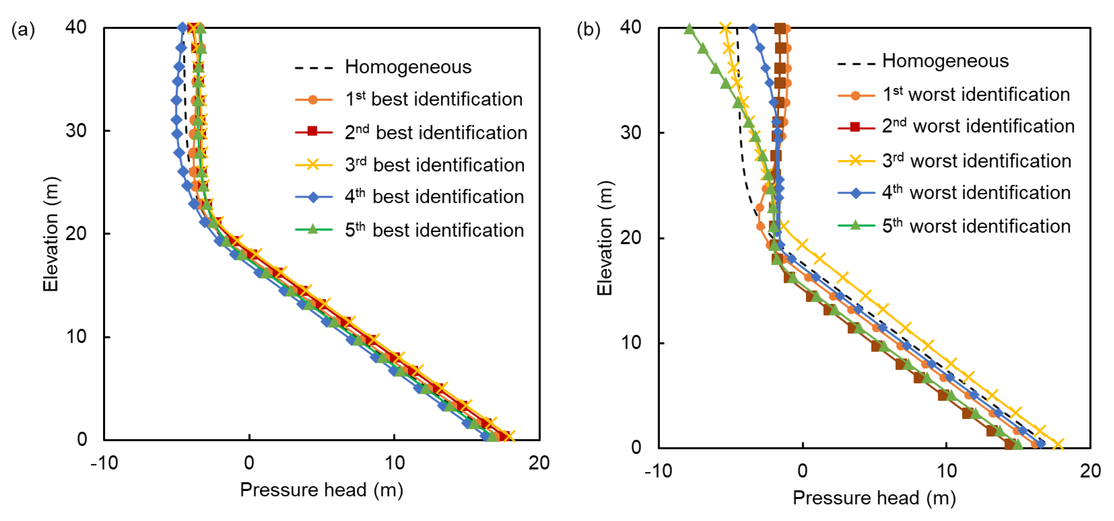
To further analyze the characteristics of the pressure head responses in these fields, Figure 10a,b show the pressure head profiles corresponding to the ten fields and the homogeneous case in section A-A of the slope (Figure 2). It can be observed that only a small deviation of pressure head profiles exists between the five best-estimated fields and the homogeneous case. This is because the ks values in the crest for the five best-estimated fields are close to the mean value (i.e., 2 × 10⁻⁵ m/s). For the worst estimated fields, the pressure head profiles in the unsaturated zones are significantly different from that of the homogeneous case. The complex responses of the pressure head may result from the less permeable zone in the slope crest.
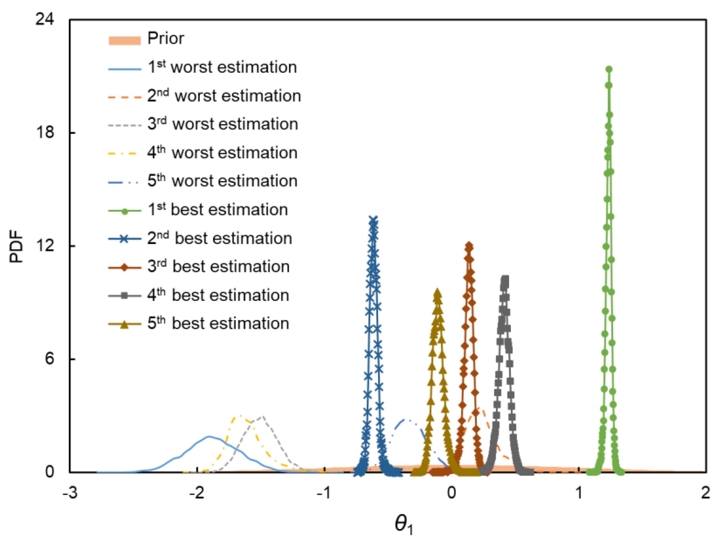
To investigate the uncertainty of random variables for Bayesian estimation, Figure 11 shows the prior and posterior distributions corresponding to the first five best and worst estimated fields of random variable θ1. Compared with the prior distribution, the posterior distributions of θ1 are within a narrower region. This indicates that θ1 corresponding to all the fields is well identified, but it is better for the first five best fields. In Table 1, the average values of the mutual information (I) for the random variables are also presented. The average I values of the best-estimated fields are nearly doubled compared with those of the worst estimated fields.
6.3. Relations between Estimation Error and Monitoring Response
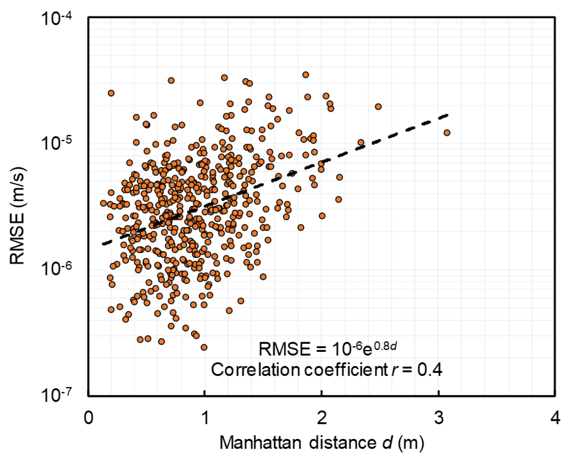
As shown in Figure 10, the performance of inverse estimation may depend on the shape of the pressure head profiles. To quantify this complexity, the metric similarity of Manhattan distance (Li et al., 2004) is introduced to qualify the shape of the pressure head profile in the A-A section (Figure 12). The pressure head profile of the homogeneous case is used as a reference. The similarity between the pressure head profile in the A-A section of 500 fields and the homogeneous case is quantified. A scatter plot of RMSE values of the 500 fields and the Manhattan distance is displayed in Figure 12. The logarithm of the RMSE values and the Manhattan distance have a positive correlation coefficient of 0.4. It implies that the pressure head profiles will cause an inaccurate estimation of soil heterogeneity. An empirical correlation equation between the Manhattan distance and the RMSE value is also given in Figure 12. This equation can be used to roughly assess the potential estimation error of the spatial heterogeneity once the pressure head monitoring data is obtained along a cross-section of the slope.
7. Conclusions
In this study, the conditions under which monitoring data can provide a more reliable estimation of hydraulic heterogeneity are investigated. The performance of the estimation is assessed based on mutual information (I) of random variables, and the root mean square error (RMSE) of the estimated field. The effect of the characteristics of heterogeneity on inverse estimation is investigated with sensitivity analysis and best-estimated and worst-estimated fields. The major conclusions of the study are summarized below.
1. The mean I value of each random variable is around two nats. All the random variables are appropriately identified, and the uncertainties are significantly reduced after inverse estimation. The RMSE corresponding to the maximum probability density is 1.77 × 10⁻⁶ m/s. The interquartile range is narrow centralized from 1.55 × 10⁻⁶ m/s to 5.67 × 10⁻⁶ m/s. The percentage error around the measurement points is less than 3%, and the COV around the measurement points is less than 0.08. The field measurements can reduce the errors and uncertainties around the locations of the monitoring points.
2. The characteristics of heterogeneity can significantly influence the effect of inverse estimation. The ranges of ks values for the best-estimated fields are much narrower than those of the worst estimated fields. For the best-estimated fields, the larger values of ks are distributed in the crest of the unsaturated zone. A less permeable crest zone could result in the complex responses of pressure head and further cause the ill identification of heterogeneity.
3. The similarity between the pressure head profiles of 500 random fields and the homogeneous case is measured. The RMSE value and the Manhattan distance have a positive correlation with a correlation coefficient r equals 0.4. It implies that the complexity of the pressure head profiles will cause an inaccurate estimation of soil heterogeneity.
One of the limitations of the present study is that the conclusions are based on numerical analysis without comparing the results to field measurements or laboratory experiments. Exploring the conditions of soil heterogeneity with real cases of field monitoring projects has several obstacles, including limited data of site investigation and measurement uncertainties. Well-controlled laboratory experiments are possible to validate the conclusions. Relevant laboratory validation is ongoing with reduced-scale slope models.
Author Contributions
Conceptualization, H.-Q.Y. and L.Z.; methodology, H.-Q.Y.; software, H.-Q.Y.; validation, J.Z., X.W. and C.T.; formal analysis, X.C.; investigation, X.C.; resources, X.C.; data curation, X.C.; writing—original draft preparation, H.-Q.Y.; writing—review and editing, L.Z.; visualization, H.-Q.Y.; supervision, L.Z.; project administration, L.Z.; funding acquisition, L.Z. All authors have read and agreed to the published version of the manuscript.
Funding
The work in this paper was supported by the Natural Science Foundation of China (Project No. 51979158, No. 51639008, No. 51679135, and No. 51422905) and the Program of Shanghai Academic Research Leader (Project No. 19XD1421900).
Acknowledgments
The authors are grateful for the support from the National Program of Changjiang Young Scholars.
Conflicts of Interest
The authors declare no conflict of interest.
References
- Schulz, W.H.; Kean, J.W.; Wang, G. Landslide movement in southwest Colorado triggered by atmospheric tides. Nat. Geosci. 2009, 2, 863–866. [Google Scholar] [CrossRef]
- Leshchinsky, B.; Olsen, M.J.; Mohney, C.; Glover-Cutter, K.; Crook, G.; Allan, J.; Bunn, M.; O’Banion, M.; Mathews, N. Mitigating coastal landslide damage. Science 2017, 357, 981–982. [Google Scholar] [CrossRef] [PubMed]
- Li, G.; Chen, G.; Li, P.; Jing, H. Efficient and accurate 3-D numerical modelling of landslide tsunami. Water 2019, 11, 2033. [Google Scholar] [CrossRef] [Green Version]
- Troncone, A.; Conte, E.; Pugliese, L. Analysis of the slope response to an increase in pore water pressure using the material point method. Water 2019, 11, 1446. [Google Scholar] [CrossRef] [Green Version]
- Kool, J.B.; Parker, J.C.; van Genuchten, M.T. Parameter estimation for unsaturated flow and transport models—A review. J. Hydrol. 1987, 91, 255–293. [Google Scholar] [CrossRef]
- Olyphant, G.A. Temporal and spatial (down profile) variability of unsaturated soil hydraulic properties determined from a combination of repeated field experiments and inverse modeling. J. Hydrol. 2003, 281, 23–35. [Google Scholar] [CrossRef]
- Guo, H.P.; Jiao, J.J. Numerical study of airflow in the unsaturated zone induced by sea tides. Water Resour. Res. 2008, 44, W06402. [Google Scholar] [CrossRef] [Green Version]
- Carsel, R.F.; Parrish, R.S. Developing joint probability distributions of soil water retention characteristics. Water Resour. Res. 1988, 24, 755–769. [Google Scholar] [CrossRef] [Green Version]
- Trandafir, A.C.; Sidle, R.C.; Gomi, T.; Kamai, T. Monitored and simulated variations in matric suction during rainfall in a residual soil slope. Environ. Geol. 2008, 55, 951–961. [Google Scholar] [CrossRef]
- Zhang, L.L.; Zheng, Y.; Zhang, L.; Li, X.; Wang, J.H. Probabilistic model calibration for soil slope under rainfall: Effects of measurement duration and frequency in field monitoring. Geotechnique 2014, 64, 365–378. [Google Scholar] [CrossRef]
- Zhang, L.L.; Zuo, Z.B.; Ye, G.L.; Jeng, D.S.; Wang, J.H. Probabilistic parameter estimation and predictive uncertainty based on field measurements for unsaturated soil slope. Comput. Geotech. 2013, 48, 72–81. [Google Scholar] [CrossRef]
- Liu, W.; Luo, X.; Huang, F.; Fu, M. Uncertainty of the soil-water characteristic curve and its effects on slope seepage and stability analysis under conditions of rainfall using the Markov Chain Monte Carlo Method. Water 2017, 9, 758. [Google Scholar] [CrossRef] [Green Version]
- Vardon, P.J.; Liu, K.; Hicks, M.A. Reduction of slope stability uncertainty based on hydraulic measurement via inverse analysis. Georisk 2016, 10, 223–240. [Google Scholar] [CrossRef]
- Gomes, G.J.; Vrugt, J.A.; Vargas, E.A., Jr.; Camargo, J.T.; Velloso, R.Q.; van Genuchten, M.T. The role of uncertainty in bedrock depth and hydraulic properties on the stability of a variably-saturated slope. Comput. Geotech. 2017, 88, 222–241. [Google Scholar] [CrossRef] [Green Version]
- Li, D.Q.; Zhang, F.P.; Cao, Z.J.; Tang, X.S.; Au, S.K. Reliability sensitivity analysis of geotechnical monitoring variables using Bayesian updating. Eng. Geol. 2018, 245, 130–140. [Google Scholar] [CrossRef]
- Yang, H.Q.; Zhang, L.L.; Li, D.Q. Efficient method for probabilistic estimation of spatially varied hydraulic properties in a soil slope based on field responses: A Bayesian approach. Comput. Geotech. 2018, 102, 262–272. [Google Scholar] [CrossRef]
- Zheng, D.; Huang, J.; Li, D.Q.; Kelly, R.; Sloan, S.W. Embankment prediction using testing data and monitored behaviour: A Bayesian updating approach. Comput. Geotech. 2018, 93, 150–162. [Google Scholar] [CrossRef]
- Nielsen, D.R. Spatial variability of field-measured soil-water properties. Hilgardia 1973, 42, 215–259. [Google Scholar] [CrossRef] [Green Version]
- Yeh, T.C.J.; Khaleel, R.; Carroll, K.C. Flow through Heterogeneous Geological Media; Cambridge University Press: Cambridge, Cambridgeshire, UK, 2015. [Google Scholar]
- Zhang, L.L.; Li, J.H.; Li, X.; Zhang, J.; Zhu, H. Rainfall-Induced Soil Slope Failure: Stability Analysis and Probabilistic Assessment; Taylor & Francis CRC Press: Boca Raton, FL, USA, 2016. [Google Scholar]
- Li, X.Y.; Zhang, L.M.; Zhu, H.; Li, J.H. Modeling geologic profiles incorporating interlayer and intralayer variabilities. J. Geotech. Geoenviron. Eng. 2018, 144, 04018047. [Google Scholar] [CrossRef]
- Lee, Y.S.; Cheuk, C.Y.; Bolton, M.D. Instability caused by a seepage impediment in layered fill slopes. Can. Geotech. J. 2008, 45, 1410–1425. [Google Scholar] [CrossRef]
- Cho, S.E. Infiltration analysis to evaluate the surficial stability of two-layered slopes considering rainfall characteristics. Eng. Geol. 2009, 105, 32–43. [Google Scholar] [CrossRef]
- Lim, K.; Li, A.J.; Lyamin, A.V. Three-dimensional slope stability assessment of two-layered undrained clay. Comput. Geotech. 2015, 70, 1–17. [Google Scholar] [CrossRef]
- Damiano, E.; Greco, R.; Guida, A.; Olivares, L.; Picarelli, L. Investigation on rainwater infiltration into layered shallow covers in pyroclastic soils and its effect on slope stability. Eng. Geol. 2017, 220, 208–218. [Google Scholar] [CrossRef]
- Wang, Y.; Huang, K.; Cao, Z. Bayesian identification of soil strata in London clay. Géotechnique 2014, 64, 239–246. [Google Scholar] [CrossRef]
- Li, J.; Cassidy, M.J.; Huang, J.; Zhang, L.; Kelly, R. Probabilistic identification of soil stratification. Geotechnique 2015, 66, 16–26. [Google Scholar] [CrossRef] [Green Version]
- Vanmarcke, E. Random Fields: Analysis and Synthesis; Revised and Expanded New Edition; World Scientific: Singapore, 2010. [Google Scholar]
- Santoso, A.M.; Phoon, K.K.; Quek, S.T. Effects of soil spatial variability on rainfall-induced landslides. Comput. Struct. 2011, 89, 893–900. [Google Scholar] [CrossRef]
- Zhu, H.; Zhang, L.M.; Zhang, L.L.; Zhou, C.B. Two-dimensional probabilistic infiltration analysis with a spatially varying permeability function. Comput. Geotech. 2013, 48, 249–259. [Google Scholar] [CrossRef]
- Cai, J.S.; Yan, E.C.; Yeh, T.C.J.; Zha, Y.Y. Effects of heterogeneity distribution on hillslope stability during rainfalls. Water Sci. Eng. 2016, 9, 134–144. [Google Scholar] [CrossRef] [Green Version]
- Marzouk, Y.M.; Najm, H.N. Dimensionality reduction and polynomial chaos acceleration of Bayesian inference in inverse problems. J. Comput. Phys. 2009, 228, 1862–1902. [Google Scholar] [CrossRef] [Green Version]
- Laloy, E.; Rogiers, B.; Vrugt, J.; Mallants, D.; Jacques, D. Efficient posterior exploration of a high-dimensional groundwater model from two-stage Markov chain Monte Carlo simulation and polynomial chaos expansion. Water Resour. Res. 2013, 49, 2664–2682. [Google Scholar] [CrossRef] [Green Version]
- Tagade, P.M.; Choi, H.L. A generalized polynomial chaos-based method for efficient Bayesian calibration of uncertain computational models. Inverse Probl. Sci. Eng. 2014, 22, 602–624. [Google Scholar] [CrossRef] [Green Version]
- Sraj, I.; Le Maître, O.P.; Knio, O.M.; Hoteit, I. Coordinate transformation and polynomial chaos for the Bayesian inference of a Gaussian process with parametrized prior covariance function. Comp. Meth. Appl. Mech. Eng. 2016, 298, 205–228. [Google Scholar] [CrossRef] [Green Version]
- Yang, H.Q.; Zhang, L.L.; Xue, J.F.; Zhang, J.; Li, X. Unsaturated soil slope characterization with Karhunen–Loève and polynomial chaos via Bayesian approach. Eng. Comput. 2019, 35, 337–350. [Google Scholar] [CrossRef]
- Zhang, L.; Wu, F.; Zhang, H.; Zhang, L.; Zhang, J. Influences of internal erosion on infiltration and slope stability. Bull. Eng. Geol. Environ. 2019, 78, 1815–1827. [Google Scholar] [CrossRef]
- Chen, X.; Zhang, L.; Chen, L.; Li, X.; Liu, D. Slope stability analysis based on the Coupled Eulerian-Lagrangian finite element method. Bull. Eng. Geol. Environ. 2019, 78, 4451–4463. [Google Scholar] [CrossRef]
- Jin, D.; Shen, X.; Yuan, D. Theoretical analysis of three-dimensional ground displacements induced by shield tunneling. Appl. Math. Model. 2019. [Google Scholar] [CrossRef]
- Jiang, S.H.; Li, D.Q.; Zhang, L.M.; Zhou, C.B. Slope reliability analysis considering spatially variable shear strength parameters using a non-intrusive stochastic finite element method. Eng. Geol. 2014, 168, 120–128. [Google Scholar] [CrossRef]
- Pan, Q.; Dias, D. Probabilistic evaluation of tunnel face stability in spatially random soils using sparse polynomial chaos expansion with global sensitivity analysis. Acta Geotech. 2017, 12, 1415–1429. [Google Scholar] [CrossRef]
- Zhang, L.L.; Zhang, J.; Zhang, L.M.; Tang, W.H. Back analysis of slope failure with Markov chain Monte Carlo simulation. Comput. Geotech. 2010, 37, 905–912. [Google Scholar] [CrossRef]
- Brooks, R.H.; Core, A.T. Hydraulic properties of porous media. In Hydrology Papers; Colorado State University: Fort Collins, CO, USA, 1964. [Google Scholar]
- Mualem, Y. A new model for predicting the hydraulic conductivity of unsaturated porous media. Water Resour. Res. 1976, 12, 513–522. [Google Scholar] [CrossRef] [Green Version]
- Van Genuchten, M.T. A closed-form equation for predicting the hydraulic conductivity of unsaturated soils. Soil Sci. Soc. Am. J. 1980, 44, 892–898. [Google Scholar] [CrossRef] [Green Version]
- Vogel, T.; Cislerova, M. On the reliability of unsaturated hydraulic conductivity calculated from the moisture retention curve. Transp. Porous Med. 1988, 3, 1–15. [Google Scholar] [CrossRef]
- Fredlund, D.G.; Rahardjo, H.; Fredlund, M.D. Unsaturated Soil Mechanics in Engineering Practice; John Wiley & Sons: Hoboken, NJ, USA, 2012. [Google Scholar]
- Leong, E.C.; Rahardjo, H. Permeability functions for unsaturated soils. J. Geotech. Geoenviron. Eng. 1997, 123, 1118–1126. [Google Scholar] [CrossRef] [Green Version]
- Fredlund, D.G.; Xing, A. Equations for the soil-water characteristic curve. Can. Geotech. J. 1994, 31, 521–532. [Google Scholar] [CrossRef]
- Johnson, K.A.; Sitar, N. Hydrologic conditions leading to debris-flow initiation. Can. Geotech. J. 1990, 27, 789–801. [Google Scholar] [CrossRef]
- Dai, F.C.; Lee, C.F.; Wang, S.J. Characterization of rainfall-induced landslides. Int. J. Remote Sens. 2003, 24, 4817–4834. [Google Scholar] [CrossRef]
- Fourie, A.B.; Rowe, D.; Blight, G.E. The effect of infiltration on the stability of the slopes of a dry ash dump. Geotechnique 1999, 49, 1–13. [Google Scholar] [CrossRef]
- Evans, N.C.; Lam, J.S. Tung Chung East Natural Terrain Study Area Ground Movement and Groundwater Monitoring Equipment and Preliminary Results; Geotechnical Engineering Office: Hong Kong, China, 2003.
- MacKay, D.J.C. Information Theory, Inference and Learning Algorithms; Cambridge University Press: Cambridge, Cambridgeshire, UK, 2003. [Google Scholar]
- Zhang, L.L.; Fredlund, D.G.; Zhang, L.M.; Tang, W.H. Numerical study of soil conditions under which matric suction can be maintained. Can. Geotech. J. 2004, 41, 569–582. [Google Scholar] [CrossRef]
Figure 1.
Spatial heterogeneity of soil: (a) Natural soil heterogeneity in the field; (b) inter-layer heterogeneity (heterogeneous in layers); (c) intra-layer heterogeneity (spatially correlated).
Figure 1.
Spatial heterogeneity of soil: (a) Natural soil heterogeneity in the field; (b) inter-layer heterogeneity (heterogeneous in layers); (c) intra-layer heterogeneity (spatially correlated).

Figure 2.
Slope model and the monitoring points.

Figure 3.
Effects of the number of realizations on the mean value of pressure head responses at the sixteen measurement points (No. is the corresponding measurement point in Figure 2).
Figure 3.
Effects of the number of realizations on the mean value of pressure head responses at the sixteen measurement points (No. is the corresponding measurement point in Figure 2).

Figure 4.
The mean I value of random variables θ1–θ6 estimated with 500 sets of synthetic monitoring data.
Figure 4.
The mean I value of random variables θ1–θ6 estimated with 500 sets of synthetic monitoring data.

Figure 5.
The probability density function (kernel smooth) of the RMSE based on 500 sets of synthetic monitoring data.
Figure 5.
The probability density function (kernel smooth) of the RMSE based on 500 sets of synthetic monitoring data.

Figure 6.
Contour map of the mean percentage error with 500 sets of synthetic monitoring data.

Figure 7.
Coefficient of variation (COV) of the estimated field with 500 sets of synthetic monitoring data.
Figure 7.
Coefficient of variation (COV) of the estimated field with 500 sets of synthetic monitoring data.

Figure 8.
Average sensitivity of pressure head at measurement points with respect to ks.

Figure 9.
Real fields: (a) First five best estimations; (b) first five worst estimations.

Figure 10.
Pressure head profile in section A-A (x = 25 m) in Figure 2: (a) First five best estimation; (b) First five worst estimation.
Figure 10.
Pressure head profile in section A-A (x = 25 m) in Figure 2: (a) First five best estimation; (b) First five worst estimation.

Figure 11.
Prior and posterior distributions of the first five best and worst estimated fields of random variable θ1.
Figure 11.
Prior and posterior distributions of the first five best and worst estimated fields of random variable θ1.

Figure 12.
Scatter plot of RMSE and Manhattan distance of pressure head in section A-A (x = 25 m) in Figure 2.
Figure 12.
Scatter plot of RMSE and Manhattan distance of pressure head in section A-A (x = 25 m) in Figure 2.


Table 1.
RMSE, average mutual information (I) with six random variables and Manhattan distance (d) of the first five best and worst estimated fields.
Table 1.
RMSE, average mutual information (I) with six random variables and Manhattan distance (d) of the first five best and worst estimated fields.
| Rank | 1st | 2nd | 3rd | 4th | 5th | |
|---|---|---|---|---|---|---|
| Best estimation | RMSE (×10−7 m/s) | 2.43 | 2.68 | 2.81 | 2.82 | 3.02 |
| Average I (nat) | 3.44 | 3.11 | 2.92 | 2.69 | 2.77 | |
| d (m) | 20.82 | 13.30 | 9.41 | 10.85 | 19.41 | |
| Worst estimation | RMSE (×10−5 m/s) | 3.49 | 3.30 | 3.17 | 3.11 | 3.00 |
| Average I (nat) | 0.93 | 1.51 | 1.62 | 1.50 | 1.55 | |
| d (m) | 39.06 | 24.48 | 15.00 | 28.40 | 29.08 |
© 2020 by the authors. Licensee MDPI, Basel, Switzerland. This article is an open access article distributed under the terms and conditions of the Creative Commons Attribution (CC BY) license (http://creativecommons.org/licenses/by/4.0/).
Share and Cite
MDPI and ACS Style
Yang, H.-Q.; Chen, X.; Zhang, L.; Zhang, J.; Wei, X.; Tang, C. Conditions of Hydraulic Heterogeneity under Which Bayesian Estimation is More Reliable. Water 2020, 12, 160. https://doi.org/10.3390/w12010160
AMA Style
Yang H-Q, Chen X, Zhang L, Zhang J, Wei X, Tang C. Conditions of Hydraulic Heterogeneity under Which Bayesian Estimation is More Reliable. Water. 2020; 12(1):160. https://doi.org/10.3390/w12010160
Chicago/Turabian StyleYang, Hao-Qing, Xiangyu Chen, Lulu Zhang, Jie Zhang, Xiao Wei, and Chong Tang. 2020. "Conditions of Hydraulic Heterogeneity under Which Bayesian Estimation is More Reliable" Water 12, no. 1: 160. https://doi.org/10.3390/w12010160
Note that from the first issue of 2016, this journal uses article numbers instead of page numbers. See further details here.