Analysis of Hyetographs for Drainage System Modeling


Department of Water Supply and Sewerage Systems, Faculty of Environmental Engineering, Wroclaw University of Science and Technology, 50-370 Wroclaw, Poland
*
Author to whom correspondence should be addressed.
Water 2020, 12(1), 149; https://doi.org/10.3390/w12010149
Submission received: 14 November 2019
/
Revised: 26 December 2019
/
Accepted: 30 December 2019
/
Published: 3 January 2020
(This article belongs to the Special Issue Innovative, Smart and Sustainable Solutions for Urban Stormwater Management)
Abstract
:Modeling the reliability of storm water drainage systems encounters a number of methodological difficulties, especially in the selection of a reliable rainfall scenario. Many methods for creating reference hyetographs are described in the literature. The aim of the work was the analysis of the shapes of local precipitation hyetographs and the verification of the reference shapes of rainfall hyetographs used for the drainage systems designing and modeling its operation in Poland (Euler type II and DVWK models). The research material was represented by historical records of rainfall data from the measuring station located in Jelenia Góra (Poland). Rainfall were grouped due to the similarity of physical features, using various methodologies: Huff, cluster analysis using the Ward and k-means methods. The k-means method proved to be especially useful for selecting precipitation in terms of shape hyetographs. The statistical analysis of the similarity of the rainfall hyetograph shapes was performed within the separated genetic clusters, based on the parameters of mass distributions and unevenness over time. The comparative analysis allowed for the positive verification of the Euler type II and DVWK models for the tested station.
1. Introduction
1.1. Drainage System Modeling
Urban floods, which are more frequent, caused by heavy rainfall and the accompanying rapid surface runoff of rainwater, cause damage, especially in urbanized areas [1]. Because of the stochastic (random) nature of precipitation, it is not entirely possible to achieve reliable operation of sewer systems. We can only strive for their safe design and operation. This translates into an adaptation of systems to the maximum forecasted streams of rainwater with the frequency of occurrence equal to the permissible frequency of spillage on the surface and flooding [2]. This also applies to future precipitation loads intensified by climate change [3,4,5,6,7].
Real environmental threats caused by floods from sewage systems can be found during their operation, while potential threats can only be demonstrated using hydrodynamic modeling. Drainage system simulation models take into account the variable (in time and space) rainfall load scenarios of the catchment, as well as the transient sewage flow in the channels. These scenarios can be both real, intense local rainfall measured over many years (generally difficult to access) and model rainfall like Euler type II or DVWK (Deutschen Verbandes für Wasserwirtschaft und Kulturbau), created on the basis of local intensity-duration-frequency curves (IDF) or depth-duration-frequency curves (DDF) of rainfall. The concept of the precipitation model defines the precipitation load with a normalized (standard) and variable course in time. Normalization is based on a statistical analysis of the history of heavy rains recorded in the past and reflects their often-repeated waveforms. Model precipitation is used in hydrological or hydrodynamic models of the rainfall-runoff phenomenon in the form of individual model precipitation or groups [8,9,10].
Modeling the reliability of sewage systems in urban areas encounters a number of methodological difficulties, requiring an urgent solution, or specifying the methodology for conducting such research. Precipitation hyetograph is a graphical representation of the intensity distribution over time. The applied hyetograph usually has a decisive impact on the simulated amount of outflow from a catchment [11,12,13]. The choice of the precipitation scenario for modeling/dimensioning drainage systems is, therefore, a significant problem. However, the diversity of actual rainfall significantly affects the uncertainty in obtaining meaningful results when modeling outflow from a drainage catchment. Hence, it is important to find a reference hyetograph that accurately reflects the typical time variability of real, local precipitation. The goal of the work is, therefore, an analysis of rainfall hyetograph shapes and verification of the reference hyetographs used for designing and modeling the drainage systems in Poland so far, using the example of the meteorological station located in Jelenia Góra.
Three genetic types of rainfall can be distinguished in the time-space structure of precipitation. The first type is convective rainfall of short-range (short-term, duration up to approximately 2 h). Then, the second type is frontal rainfall with a long-range (usually 2 to 12 h). The last type is low-pressure of a regional-scale range (long-lasting, usually more than 12 h). For dimensioning rainwater or a combined sewage system, the most important are intensive rainfalls with a duration limited to the flow time in the sewers (usually up to several hours) [5,8,14].
The most important problem when designing and modeling the drainage systems is the selection of a reliable rainfall scenario [8,15,16,17]. The use of an appropriate scenario requires the designer to determine the basic parameters of the rain, i.e., duration (t), height (h), or intensity (i). These parameters are usually determined for separate and random precipitation events.
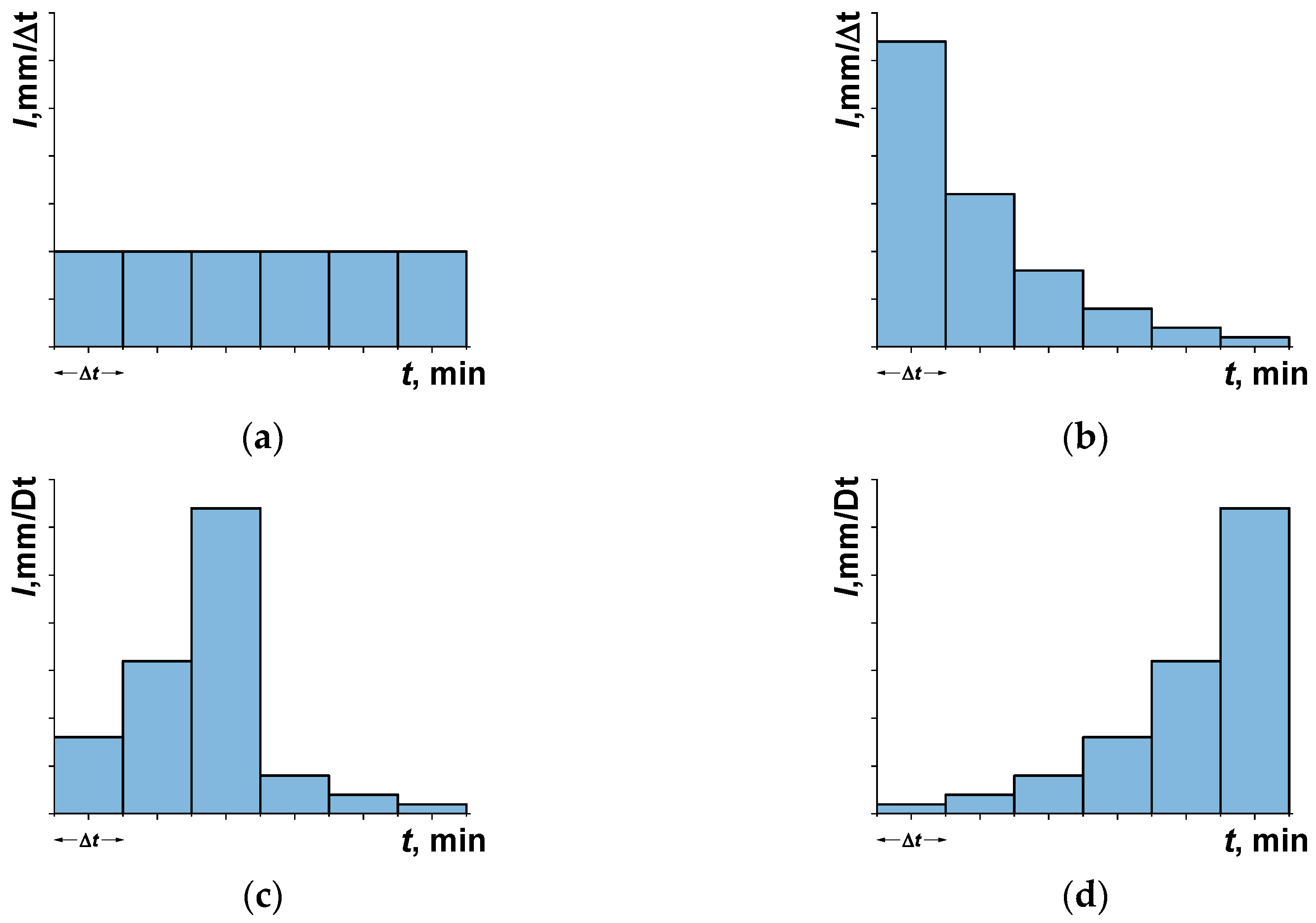
In Polish literature, there are few papers on the distribution of rainfall intensity in time and space, especially for the needs of modeling drainage of urbanized areas. Hence, typical distribution is usually adapted based on many years of rainfall observations in other countries, e.g., according to German DVWK [16] or ATV (Abwassertechnische Vereinigung) [8], or American SCS (Soil Conservation Service) [18]. According to the German guidelines [16], four typical intensity distributions in time are distinguished (Figure 1).
1.2. Reference Hyetographs
Many methods for creating reference hyetographs are described in the literature [19]. The division of these methods has been described in many works, including Chow et al. [20], Lin et al. [21], Venezziano and Villani [22], or S. Cazanescu and Cazanescu [23]. These methods can be generally divided into three main groups: methods based on IDF/DDF curves, methods based on historical rainfall data, and stochastic methods.
Standard hyetographs based on IDF curves belong to the oldest group of methods for creating model precipitation. These methods can be further divided into two subgroups: methods based on a single point of the IDF curve and methods based on the entire IDF curve. Each of the methods belonging to the first subgroup is based on the precipitation height/intensity reading from the DDF/IDF curve for a given duration and frequency of precipitation, and then, in a sense, selecting a “random” distribution to create a reference hyetograph [22,24]. Methods based on a single point of the IDF curve include hyetograph with simple geometric shapes. The most known representatives are block hyetographs. They have a shape of rectangular and characteristic rainfall with constant intensity over time. Precipitation of this type is commonly used for dimensioning sewage systems (stormwater and combined) with flow time methods [8,12]. Yen and Chow [25] proposed a triangular shape of a hyetograph to reflect the “geometry” of local precipitation for small drainage systems. The triangular hyetograph pattern was also proposed by Ball, cited in Reference [26], for cases when the maximum precipitation intensity occurs either at the beginning or end of its duration. Triangular hyetographs are especially recommended for areas with a dry climate [27]. Additionally, hyetographs of other shapes are proposed in literature, including those made of several simple, geometric figures. These include, for example, the trapezoidal hyetograph proposed by Sifald in 1973 [28] and the hyetograph composed of three “triangles” proposed by Desbordes in 1978 [29], with a peak of precipitation intensity located in the central triangle (isosceles with an acute angle of aperture) and the other two, which represents precipitation before and after the peak. Lee and Ho [30] proposed the use of a “double” triangle shape hyetograph to describe rainfall in Taiwan. A simplified version of the Desbordes model [29] was presented by Peyron et al. [31] who proposed that the preceding and following parts of the peak should be in a block rather than a triangular form.
The second subgroup consists of methods based on the entire IDF curve. The best known in this case is the methodology proposed by Keifer and Chu in 1957 [32], called the “Chicago” method. The hyetograph created on the basis of the Keifer and Chu methodology is continuous. It is characterized by variable, temporary rainfall intensity and one peak of maximum value. This peak divides the hyetograph into two independent parts (branches): ascending and descending. Two parameters are important here including time to peak (the duration from the rainfall beginning to the occurrence of the peak), and time after the peak (the duration from the moment of the peak to the end of precipitation).
The previously mentioned Keifer and Chu in their research [32] for the Chicago area determined the average value of the location of the peak at r = 0.375, as representative of the rainfall durations considered t ∈ {15, 30, 60, 120} min. Hyetograph created on the basis of the Keifer and Chu methodology has a continuous form. Therefore, it is not suitable directly for application in rainfall-runoff modeling using existing application programs, where a discrete form of hyetographs (interval intensity) is required.
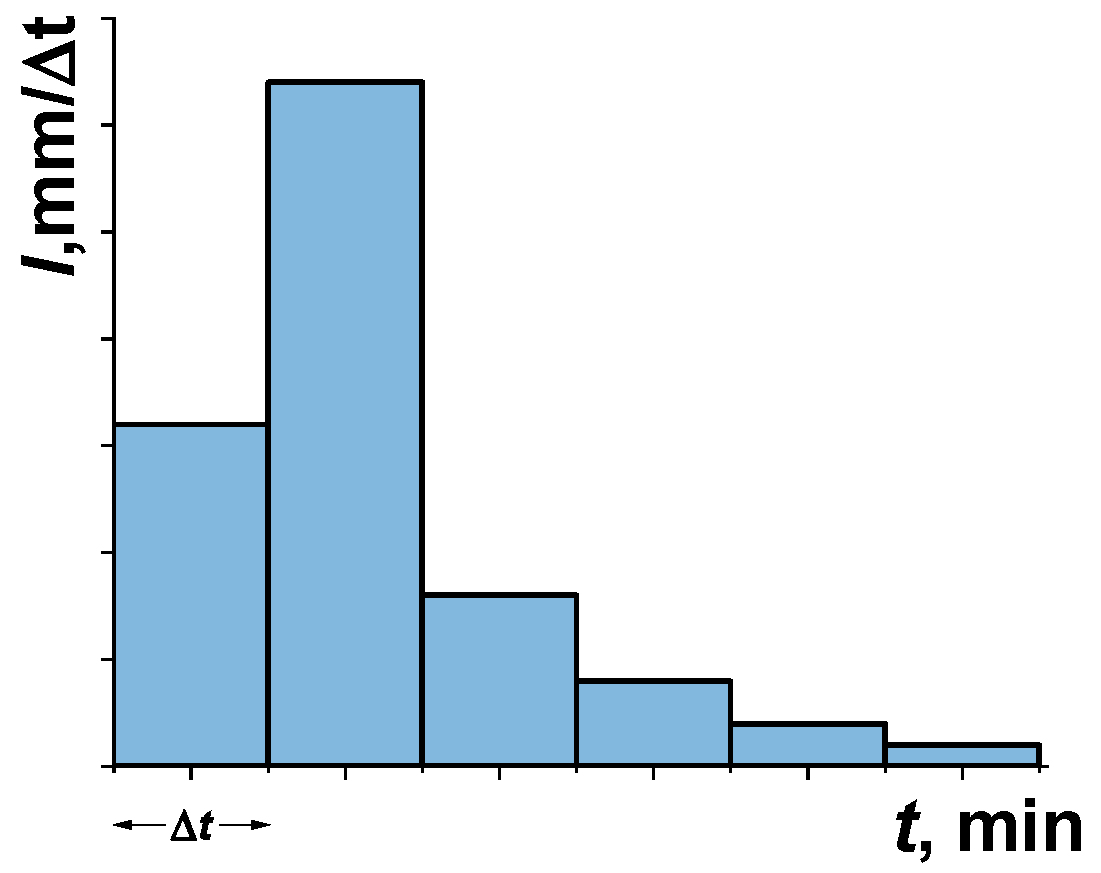
No less popular example of the reference hyetograph (from the group of methods based on whole IDF curves) is the Euler type II model (Figure 2). This model is a discrete form and is recommended for modeling sewage systems in Germany [8], as well as in Poland [12,33,34], in the presumption that Polish climatic conditions are similar to German [35]. However, the shape of the Euler type II reference hyetograph was not subjected to appropriate verification in Polish climatic conditions, which will be done in this paper. This model is based on the assumption that the largest instantaneous (Δt) precipitation intensity occurs at the end of one-third of its duration. For creating model precipitation with a five-minute discretization step (Δt = 5 min), the precipitation with the highest interval intensity is determined from the beginning of DDF/IDF curves. It is read for a given frequency of occurrence (C), located at the end of one-third of the initial duration of the model precipitation. Subsequent, lower intensities are ranked in a descending order to the left of the range with the highest intensity until the time of precipitation start is reached. The remaining, even lower range intensities are also ranked in a descending order to the right of the range with the highest intensity until reaching the end of precipitation. Usually, for the first one-third of the model rainfall duration (i.e., 33% t), approximately 70% of the total precipitation amount occurs.
The second group of methods for creating reference hyetographs are methods based on historical rainfall records. Hyetographs in this group are created by statistical analysis of data on selected precipitation phenomena [21,22,24]. They are usually presented in the form of a cumulative hyetograph, called dimensionless mass curves. These curves are a graphical representation of the relationship between the relative amount of precipitation and its duration. The best known is the method proposed by Huff in Reference [36] from 1967. Huff used precipitation data from a 12-year period (1955–1966) from 49 rain gauges in a 1037 km2 prairie area, in the eastern part of the state of Illinois (USA). He chose precipitation for durations from 1 to 48 h. Based on preliminary analyses, Huff divided precipitation events into four groups, called quartiles. This determines which part of the duration of precipitation its maximum intensity occurred (each group determines another 25% of the duration of precipitation). Based on this division he created for each group, the quartile charts illustrating changes in the amount of precipitation over time are characteristic of these groups. Huff curves are, therefore, a probabilistic representation of the ratio of cumulative precipitation heights to the corresponding cumulative durations (expressed as dimensionless) in the form of probability isopleths. Huff curves have found widespread use to analyze the variability of precipitation over time, performed, among others by Bonta and Rao [37], Pani and Haragan [38], Terranova and Iaquinta [39], Elfeki et al. [40], and Pan et al. [41]. Bonta at work [42] from 2004, presented in detail the methodology for creating Huff mass curves. Bonta also analyzed other factors affecting the construction and use of Huff curves, including the sensitivity of the shape of the curves to the data sampling interval, the impact of minimum rainfall heights selected for analysis, the minimum sample size, or the shape of the curves depending on the season.
Another method that has also found a practical application is the dimensionless mass curves method recommended by the SCS [18]. This method suggests types of rain height distributions over time, depending on the US region. Many works refer to SCS curves, including Awadallah et al. [43].
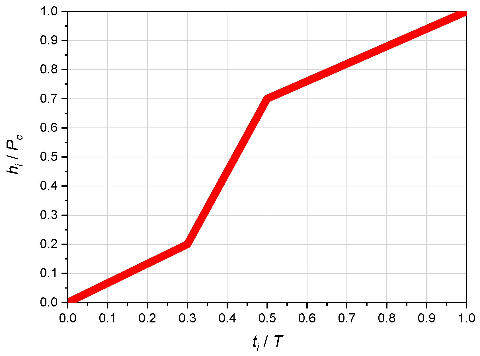
According to German guidelines DVWK [16] from 1984, a model rainfall with maximum intensity in the middle of the event should be taken as the reliable rainfall distribution (mainly for hydrological calculations of small urbanized and uncontrolled catchments). The dimensionless sum curve of this distribution is shown in Figure 3. This model is often used in Poland [44].
According to the course of the sum curve for the first 30% of the duration, precipitation will occur in 20% of its total amount. After half the duration, 70% will appear, and the remaining 30% of the total precipitation will occur in the second half of the duration. This distribution is similar to SCS type II distribution.
In the literature, you can also find many other, less known methods that present precipitation distribution in the form of dimensionless curves, including in the works of Powell et al. [45] from 2007, Vandenberghe et al. [46] from 2010, or Terranova and Iaquetta [39] from 2011. To date, mass curves have been used mainly for modeling small, uncontrolled river basins, and rarely for modeling urbanized catchments [47].
Analysis of rainfall time variability for the purposes of creating reliable reference hyetographs is of interest to many researchers. In the current studies, precipitation data were divided into groups according to their duration (the genetic type of precipitation). Often, for each group (t), separate reference hyetographs were created. However, there are no studies that would take into account the frequency (C) of occurrence of given precipitation (with exceedance), which is necessary for the application to model the reliability of a sewage system operation. At the same time, parameters of the hyetograph describing unevenness in time are not specified, which should be taken into account when comparing their shapes.
2. Method of Analysis
Unevenness of precipitation parameters over time (e.g., h, i, and q) can be determined and compared in individual groups of their durations, respectively: convective, frontal, and low-pressure, i.e., in the scope of t ∈ [10, 120] min, t ∈ (120, 720] min, and t > 720 min. Frequency of occurrence: C ∈ {1, 2, 5, 10} years, as most commonly used for dimensioning and modeling of sewage systems (according to ATV/DWA-A118: 2006 and PN-EN 752: 2017) should be considered. This is synonymous with the need to analyze the shapes of local hyetographs taking into account the exceedance frequency classes (C ∈ {≥1, ≥2, ≥5, ≥10} years).
Precipitation hyetograph can be characterized in terms of unevenness in time by two geometric indicators:
- ▪
- location of the interval Δt with the cut off (tpeak) peak of maximum precipitation hmax(Δt),
- ▪
- location of the interval Δt with the cut off (tcg) of the center of gravity of the hyetograph Pc/2,
for a variable (dimensionless systems) or constant (dimensional systems) step discretization time Δt, defined as:
where: r—peak position ratio for the maximum interval precipitation height (hmax(Δt)), tpeak(hmax(Δt))—the time of peak interval precipitation, min, T—total duration of rainfall, min, rcg—hyetograph center of the gravity position indicator, tcg(Pc ÷ 2)—time of the center of gravity of the hyetograph (for Pc ÷ 2), min, Pc—cumulative (total) rainfall amount (in time T), mm.
For the needs of mass hyetographs in dimensionless systems (Euler type II or DVWK), a fixed number of 10 intervals Δt was assumed, which allows us to position the peak/peaks (r) of the maximum interval height (intensity) of precipitation, with an accuracy of 0.1T. This forces the use of different, discretely set values of time intervals: Δt ∈ {1.0 min (for T = 10 min), 1.5 min (T = 15 min), 2.0 min (T = 20 min), … 5.0 min (T = 50 min), … 144 min (T = 1440 min), … 432 min (T = 4320 min)}. For the purposes of creating rainfall hyetographs in dimensional systems, a fixed value of the time interval will be used: Δt = 5.0 min (as in the Euler type II model), which, for convective precipitation, determines the variable number of intervals Δt (e.g., 24 for t = 120 min).
For the description and analysis of mass distribution on hyetographs (rainfall height distribution over time), five mass indicators were defined.
- ▪
- m1—as the cumulative ratio of precipitation height (mass) for the time from t = 0 to t = tpeak (before the cut off peak of maximum rainfall hmax(Δt)), to the cumulative amount of precipitation for the time from t = tpeak down t = T (by peak):
- ▪
- m2—as the ratio of the maximum interval height (mass) of precipitation to the total height:
- ▪
- m3—as the ratio of the accumulated height (mass) of precipitation for the time from t = 0 to t = 0.33T, to the total height.
- ▪
- m4—as the ratio of the accumulated height (mass) of precipitation for the time from t = 0 to t = 0.3T, to the total height.
- ▪
- m5—as the ratio of the accumulated height (mass) of precipitation for the time from t = 0 to t = 0.5T, to the total height.where m1, m2, m3, m4, and m5—mass distribution ratios on a hyetograph (sum of rainfall amounts), hi—instantaneous height of rainfall (for Δt = 1 min), mm, hmax(Δt)—maximum interval (Δt) precipitation height, mm, Pc(T)—total rainfall height (in time T), mm, 0.33T—first one-third of the total rainfall duration (T), min, 0.3T—the first 30% of the total rainfall duration (T), min, and 0.5T—the first 50% of the total rainfall duration (T), min.
To describe unevenness of intensity (i), an indicator was defined as the ratio of the maximum interval value to the average value from the entire duration of the precipitation (T), i.e., respectively.
where: ni—indicator of rainfall intensity irregularity over time, imax(Δt)—maximum interval (Δt) rainfall intensity, mm/min, and im (T)—mean rainfall intensity (over time T), mm/min.
Some of the indicators (r, rcg, m1, m2, m4, and m5) are especially dedicated to the analysis of similarity of mass hyetographs in dimensionless systems (variable value Δt = 0.1T) for the DVWK pattern. The remaining two indicators (m3 and ni) are dedicated to comparative analyses of shapes of real precipitation hygrographs in dimensional systems (Δt = const = 5 min). In particular, the indicator m3, according to Formula (5), is intended for analyses of the similarity of convective precipitation hyetographs to a Euler type II pattern.
3. Study Area and Data Used
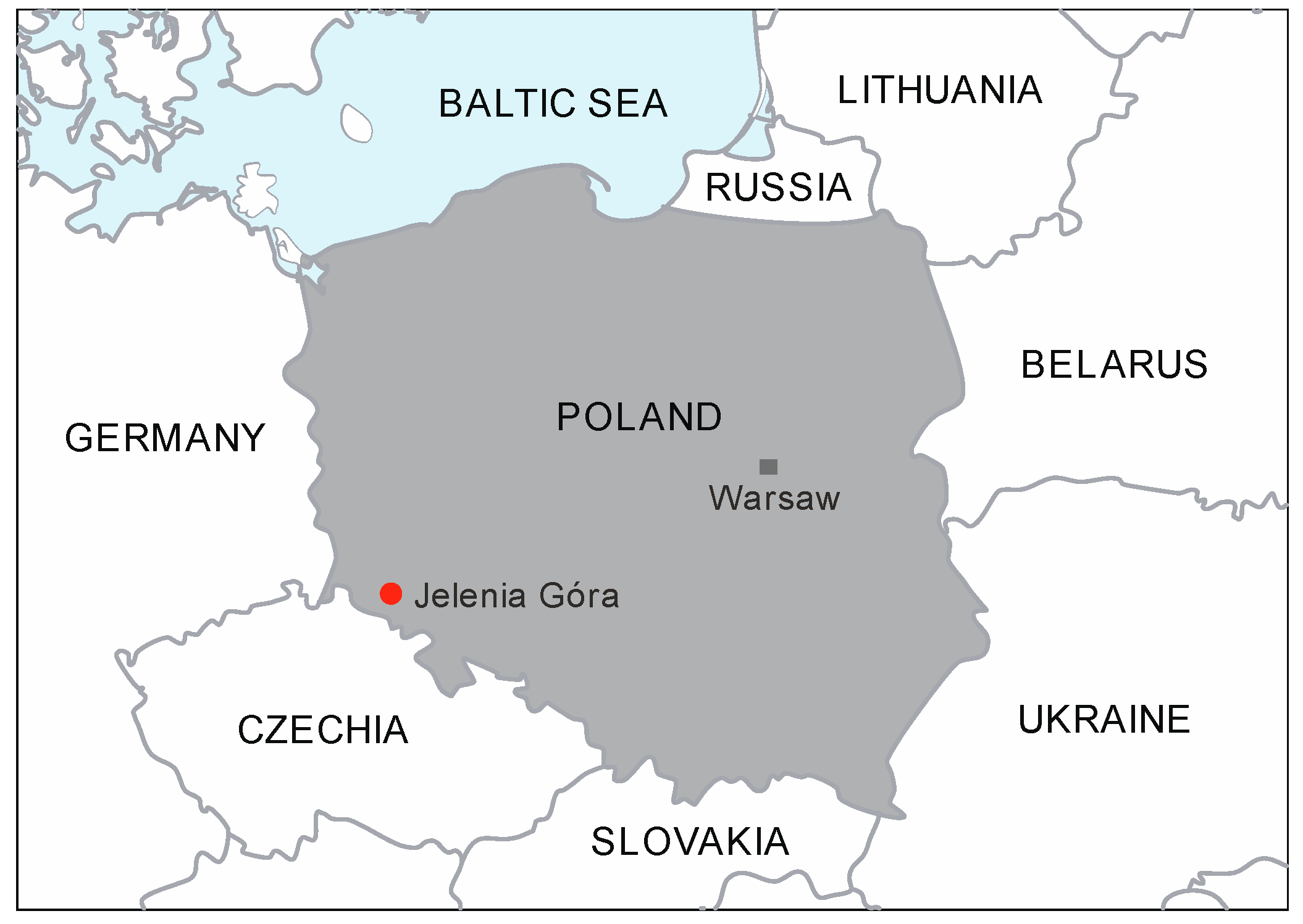
The research material is historical records of precipitation data from one of the measuring stations of the Institute of Meteorology and Water Management—National Research Institute (IMGW-PIB), located in Jelenia Góra. The station is placed at an altitude of 342 m a.s.l. and has high maximum values of daily precipitation sums (119.3 mm). The location of the station is shown in Figure 4.
For several years (since 2005), precipitation data on the IMGW-PIB meteorological stations are recorded using electronic rain gauges—RG-50, by SEBA Hydrometrie GmbH & Co. KG KG. Rain gauges are equipped with a heating system. They can, therefore, record rainfall not only during periods of positive temperatures (May–October) but also in the months of the cold hydrological half-year (November–April). Available data strings from rainfall registration at the IMGW-PIB Jelenia Góra station fall in the period 1960–2008 (registration on paper strips) and 2005–2018 (electronic registration), which, in total, translates into 59 years of a continuous rainfall observation. A separate set of precipitation data was used to study the shapes of hyetographs registered with a time step of 1 minute in the period of 2005–2018.
For the selection of independent precipitation due to their frequency of occurrence: C ∈ {1, 2, 5, 10} years, the physical model of maximum precipitation for Jelenia Góra, developed on the basis of rainfall data from 1968–2017, was used.
applicable to: t ∈ [10, 1440] min and C ∈ [1, 50] years and necessary to determine the threshold values for precipitation h(t, C) as the baseline for attributing the appropriate frequency of precipitation (C). On this basis, the rainfall statistical analysis selected precipitation of exceedance frequencies C(T) ≥ 1 year, obtaining a population of 80 rainfall, which was grouped by duration into three groups (seven subgroups). Then, due to the occurrence frequency, precipitation was classified into four classes of exceedance rate. The amount of precipitation in individual groups of both classifications is summarized in Table 1.
4. Results and Discussion
4.1. Grouping Precipitation for Statistical Analysis
4.1.1. Huff’s Method
For the purpose of examining the shapes of dimensionless mass hyetographs, a discrete value of the time interval Δt(T) was determined in which the increase in precipitation height will be analyzed. The time step established for each of the selected precipitation had to meet the condition of obtaining 10 intervals: Δt ϵ {1.0 min (for T = 10 min); 1.5 min (for T = 15 min); 2.0 min (for T = 20 min); … 144 (for T = 1440 min); … 432 min (for T = 4320 min)}. Then, for each time interval Δt, representing 10% (0.1T) of the total duration of precipitation, cumulative rainfall heights were determined hi/Pc ≡ P/Pc—for cumulative durations ti/T. First, the Huff methodology was used to analyze the similarity of the shapes of the examined hyetographs. Huff curves are based on the division of precipitation into four groups—quartiles depending on the part of the duration, which occurred as the largest amount (mass gain). According to this division method, precipitation increases in each of the 25% of the rainfall duration, which were determined for each of the analyzed precipitation. The rainfall were assigned to four quartile groups on this basis.
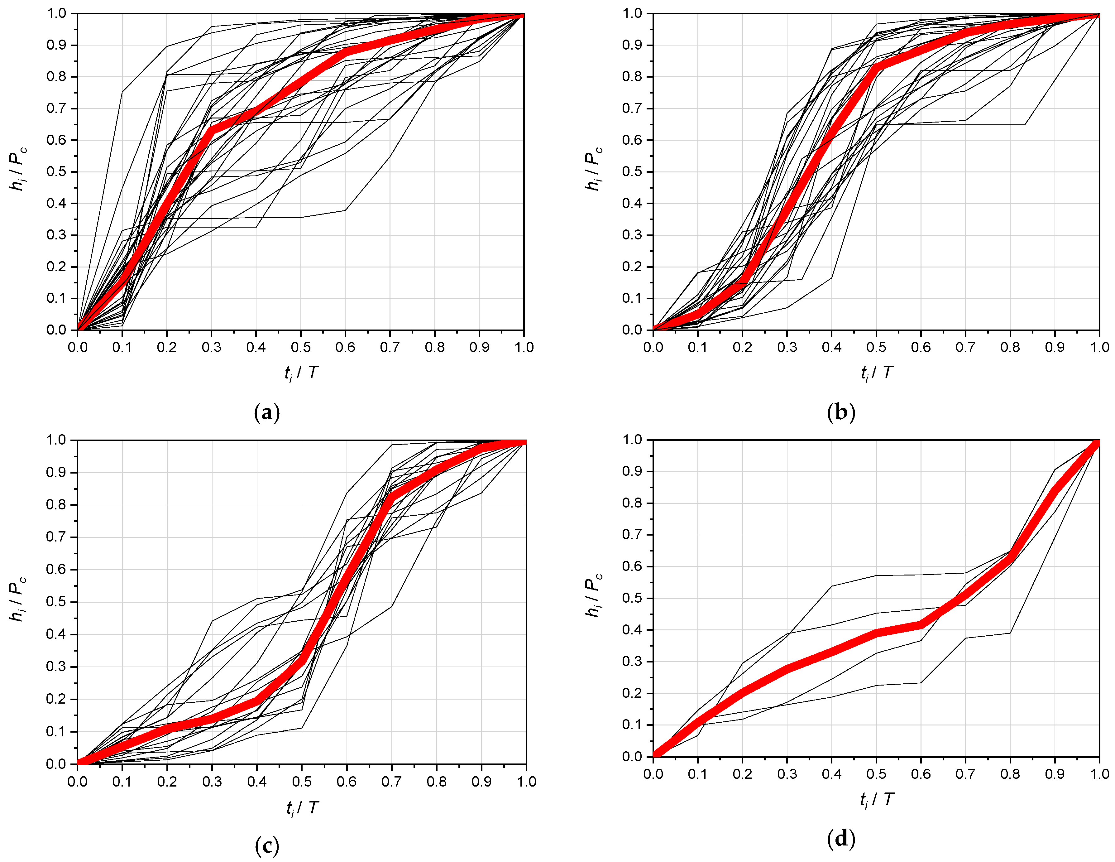
As a result, the 80 tested precipitations were assigned to Huff groups I, II, III, and IV in the following order: 30 (37%), 27 (34%), 19 (24%), and 4 (5% of the population). It can be seen that the largest population of the analyzed phenomena are precipitation from the I and II quartile group (71%), which means that the vast majority of precipitation mass increase is concentrated in the first half of its duration. For each quartile group, the associated sum curves with the calculated median curve are illustrated (Figure 5).
In each of the received quartile groups, the amount of precipitation was examined in individual duration groups as well as in the frequency classes of exceedance. Generally, for convective (29% of the population) and frontal (49%) precipitation, a significant numerical superiority of their occurrence was observed in quartile groups I and II (61%), where the largest increase in precipitation occurs in the first half of the duration. Low-pressure rainfall (22% of the population), i.e., duration t > 720 min, occurs in all quartile groups. In the least numerous IV quartile group, there are mainly low-pressure rainfall (three from the subgroup t ∈ (720, 1440] min).
The above results of preliminary analyses confirm the general conclusions of Huff’s studies [36,48,49] that the largest rainfall population (71%) occurs in the first and second quartile groups. The grouping of rainfall population in Jelenia Góra with the Huff’s method confirmed the observations that precipitation with durations T ≤ 360 min tend to be more often associated with the distribution, according to the first quartile (42%), while precipitation by T ∈ (360, 720] min most often belong to the second quartile (43%). For precipitation with longer durations, Huff’s regularity was no longer confirmed that for T ∈ (720, 1440] min precipitation usually have a distribution characteristic of the third quartile (in Jelenia Góra are evenly spaced in four quartiles) and the precipitation of T > 1440 min most often have the distribution of the fourth quartile (in Jelenia Góra, they predominate in the third quartile). The results of the above analyses clearly indicate the randomness of the tested precipitation phenomena.
In the case of rainfall analysis in four classes of exceedance frequencies (Table 2), one can notice a numerical superiority of precipitation included in the I or II quartile group, respectively, with 30 precipitation (37% of the population) and 27 precipitation (34%) in relation to other quartile groups. In particular, in class I of the frequency of exceedance, i.e., for C ∈ [1, 2) years, comprising 26 precipitation (33% of events), the number of precipitation in the first quartile group prevails—14 precipitation, i.e., 54%. In the separated class II of the frequency of exceedance, i.e., for C ∈ [2, 5) years, covering 24 precipitation (30% of the population), precipitation in the I and II quarter groups predominate, with 8 and 10 precipitation, respectively, i.e., 33% and 42%. In the III class of the exceedance frequency—for C ∈ [5, 10) years, comprising only nine precipitations (11% of the total population), the number of precipitations in the I quarter group prevails—4, i.e., 44%. In class IV of the exceedance frequency tested, among the precipitation by C ≥ 10 years, comprising 21 events (26% of the population), are prevailing in precipitation already included in the II or III quartile group—10 and 7 precipitation, respectively, i.e., 48% and 33% (Table 2).
Grouping of precipitation by the Huff method, even though it allows the detection of interesting general hydrological relationships, it does not allow the determination of clear “patterns” of examined mass hyetographs/histograms, which both depend on the duration of precipitation and the frequency of occurrence. Shapes of dimensionless hyetographs in the form of sum curves of precipitation heights (Figure 5) in Huff’s quartile groups are quite irregular. However, the mass distribution of the hyetograph in the first quartile group is most similar to the Euler type II standard, wherein one-third of the initial duration of precipitation with approximately two-thirds of its weight is deposed. In contrast, the second quartile group approximately reflects the mass distribution, according to the DVWK pattern, where 20% of its precipitation is deposited on 30% of the initial duration of the precipitation, and on 50% T—already 70% by mass [16,50].
4.1.2. Cluster Analysis Using the Ward Method
For the purpose of the work, an attempt was made to examine in detail the similarity features of the shapes of rainfall hyetographs in groups (and subgroups) of their duration, taking into account the exceedance frequency classes. First, cluster analysis using the Ward method was used to extract homogeneous, similar subsets of the objects of the studied population. The measure of similarity is the function of the bond distance of object pairs. Most of the Euclidean distance is used, i.e., the geometric distance in the multi-dimensional space of the form [51].
where xi and yi are the values of cumulative rainfall amounts of the examined rainfall x and y, and p is the number of rainfalls tested.
The Ward method belongs to the hierarchical methods in which each object is a separate cluster and then viewed lying nearest to each other, which are combined into a new cluster until one cluster. The error sum of squares is a measure of the diversity of the cluster relative to the mean values, determined from the formula.
where: xi—value of the cumulative rainfall amount being the segmentation criterion for i rainfall, k—number of objects in focus.
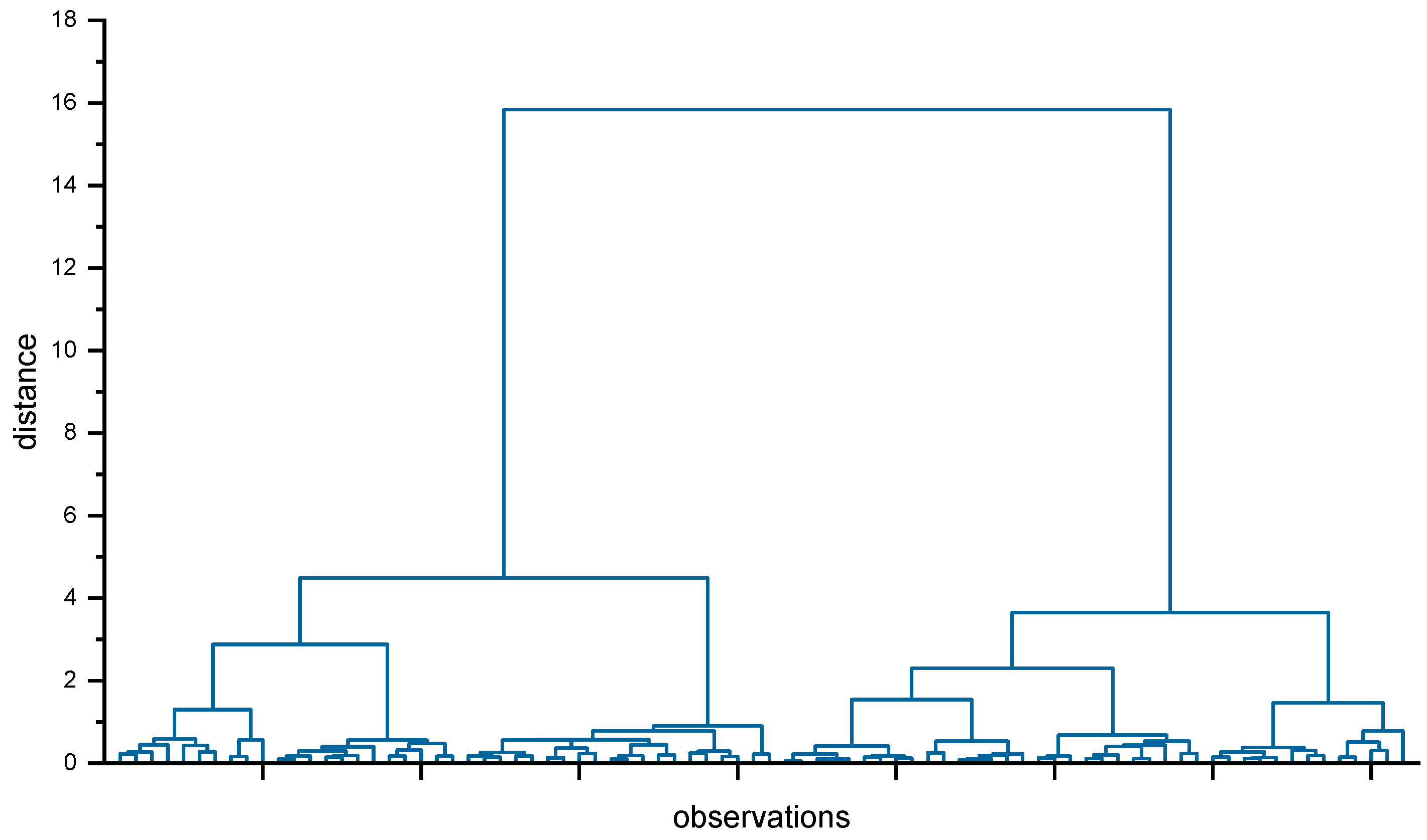
Figure 6 presents the dendrogram resulting from the grouping of the analyzed 80 precipitation shapes from the IMGW-PIB station in Jelenia Góra. The analysis of the chart made it possible to determine the cut-off distance of approximately 3, which led to the division of precipitation into four clusters with clearly different courses of intensity changes over time.
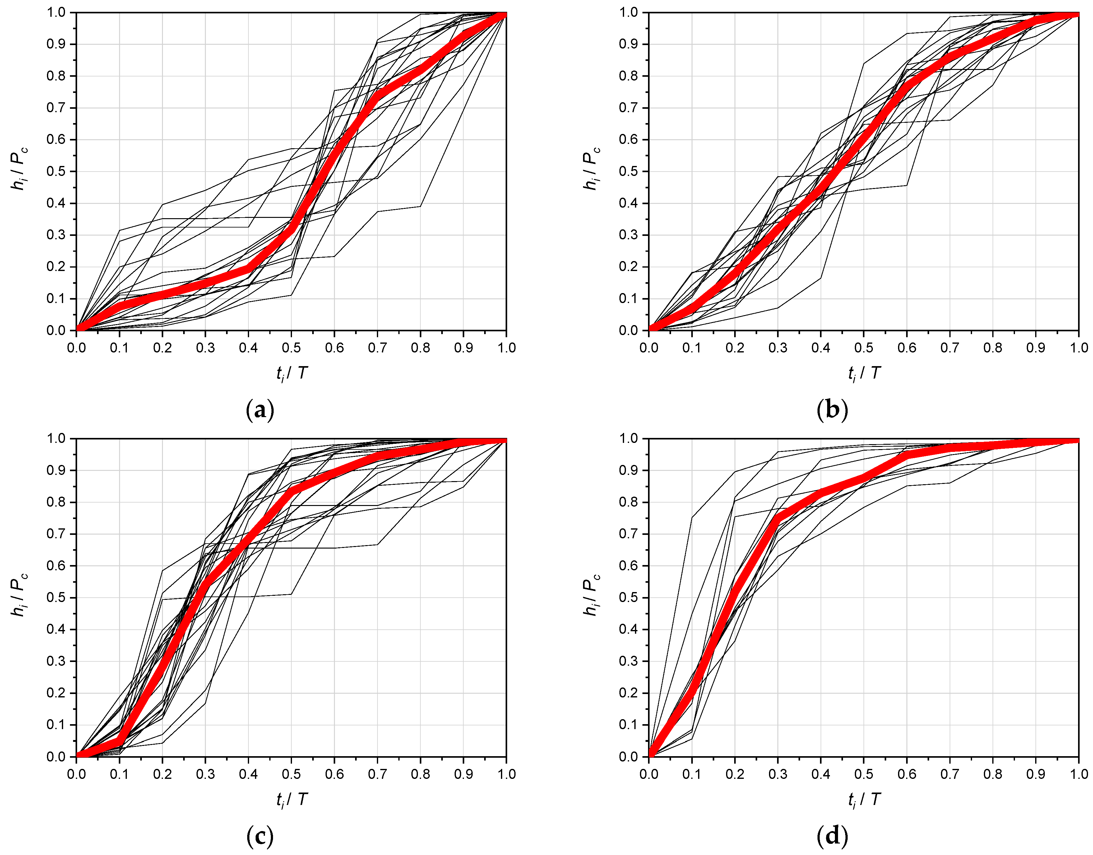
Figure 7 shows the total rainfall curves belonging to four clusters created by the Ward method, with median curves plotted. Cluster group numbers were given from the dendrogram shown in Figure 6 from left to right.
The most numerous cluster No. 3 covers 34% of the analyzed precipitation phenomena. Precipitation belonging to this cluster is characterized by maximum height increases occurring in the first half of their duration. Cluster No. 1 (26% of observations) is the second-largest, in which maximum height increases occur in the second half of the duration. Cluster No. 2 has a similar proportion (25%), but the rainfall belonging to this cluster has a similar, even course, without significant changes in intensity over time. Cluster 4 is characterized by the largest increases in the median interval. This, despite the small share of this cluster in the whole set (15%), makes them the most important among the analyzed groups for practical reasons including creating precipitation patterns (Euler type) for modeling sewage systems. However, the DVWK pattern was not clearly mapped in any of the clusters.
4.1.3. Cluster Analysis Using the Method of k-Means
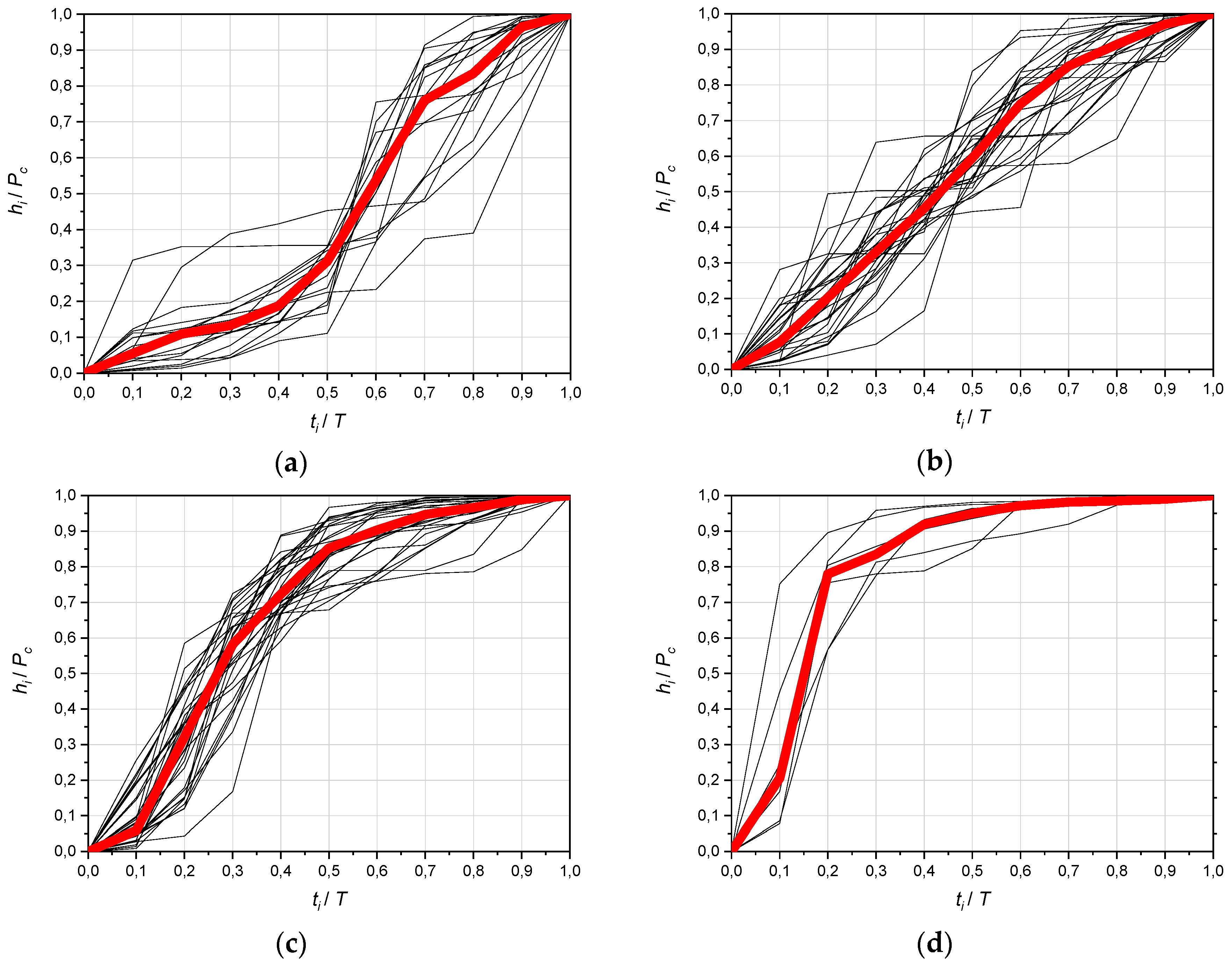
The results of agglomeration of 80 precipitation using the Ward method showed the existence of four clusters with similar runs of sum curves (dimensionless hyetographs) within the selected groups. This allows using another method of grouping precipitation—the method of k-means. This method consists of dividing the population into a predetermined number of clusters, and the obtained division is improved during the agglomeration procedure, which moves objects between them so as to obtain the minimum variance inside each of them. For grouping precipitation using the method of k-means, the number of clusters was assumed k = 4. Figure 8 shows the sum curves of precipitation in 4 on the graphs—new clusters separated by the method k-means, together with the median curves plotted.
As a result of grouping of precipitation by this method, more expressive clusters were obtained compared to the results of grouping by the Ward method. The bundles of most precipitation sum curves are closer to the respective medians in the four analyzed clusters.
In the case of precipitation grouping by the k-means method, the most numerous cluster is group 3, covering 38% (30 precipitations) of the analyzed population. The mass distribution on hyetographs belonging to this cluster is similar to the Euler type II standard, where, in one-third of the initial duration of precipitation, approximately two-thirds of its weight is deposed. Cluster No. 2 covering 34% of the population (27 precipitation) is the second largest. Precipitation belonging to this cluster is characterized by a relatively even course of changes in height over time (without clear peaks). Precipitation belonging to cluster No. 1, in the number 17 (21% of the population), has peaks of intensity increase. This is shifted to the second half of the duration. Precipitation belonging to cluster 4, with the smallest number 6 (7% of the population), has peaks of intensity increase, which is located in the first one-fifth of the duration (Figure 8). However, cluster No. 4 has the highest numerical value of the peak of relative increment, interval median height (hi/Pc = 0.575—almost six times bigger than the average hi /Pc = 0.1). In turn, that makes it similar in this respect to the Euler model precipitation (as a model for modeling stormwater drainage).
This method also resulted in more expressive median peaks in three clusters: No. 1 (hi/Pc = 0.23), No. 3 (hi/Pc = 0.27), and No. 4 (hi/Pc = 0.575) with their relative position: r = ti/T ≈ (0.6–0.7) for cluster No. 1, r ≈ (0.2–0.3) for cluster No. 3, and r ≈ 0.2 for cluster No. 4. Whereas, for cluster No. 2, the most aligned course of relative rainfall heights (on an average level: hi/Pc = 0.1) during (T). Method k-means, therefore, gives qualitatively better results of rainfall grouping compared to the Ward method.
In each of the clusters created by the k-means method, the number of precipitations was also analyzed in individual groups of durations, taking into account the exceedance frequency classes. In this respect, for the four clusters analyzed, there are no clear relationships, which only emphasizes the randomness of the phenomena studied.
The results of precipitation grouping using the k-means cluster analysis allowed for initial verification of relative position (r) peaks of the largest, interval height (intensity) of precipitation. It is important for creating precipitation patterns for modeling the operation of drainage systems. It was shown (Figure 8) that almost half of the analyzed rainfall (45% of the population) has a peak of cumulative (average) height located at one-third of the initial duration (clusters 3 and 4) during which over two-thirds of the height (mass) is deposited with total rainfall. Therefore, the features of mass distribution on dimensionless hyetographs belonging to the clusters No. 3 and 4 are similar to the Euler type II model. Clusters 3 and 4 include the majority (15) of convective precipitation (C) and the majority (10) of frontal precipitation (F) from the border between C and F, i.e., T ≤ 180 min, which is particularly important for modeling drainage in urban areas. These precipitations will, therefore, be subjected to a detailed quantitative analysis of the similarity of the histogram shapes to the Euler type II pattern.
In turn, frontal and low-pressure rainfall can be used to verify the DVWK pattern. Thus, they will be subjected to a detailed quantitative analysis of the similarity of dimensionless shapes of hyetographs to the literature pattern, where, for the first 30% of the duration of precipitation, there is 20% of its total amount. In the middle of the duration, it appears as 70%, and the remaining 30% of the total amount occurs in the second half of the duration (i.e., at 50% T) [16,50]. Neither cluster analysis using the Ward method or the method of k-means did not indicate such specific features of mass distribution on dimensionless hyetographs. However, precipitation distribution by the Huff method clearly indicated the II quartile group (Figure 5) similar in shape to the DVWK rainfall pattern. This group includes 13 precipitations, respectively: 10 F with T > 180 min and 3 L > 720 min.
4.2. Models Verification
4.2.1. Verification of Euler Type II Pattern
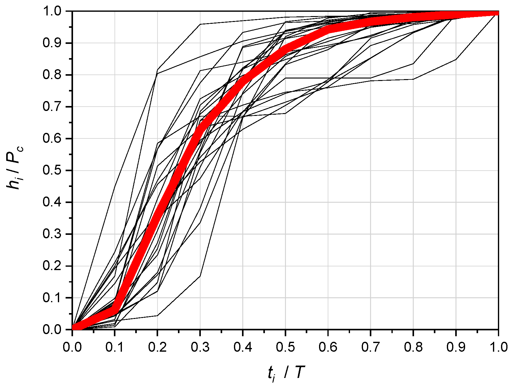
In clusters No. 3 and No. 4, there are, respectively, 13 and 2—total 15 convective precipitation, out of a total of 23 C, which is two-thirds (65%) of the C rainfall population. Of the frontal precipitation (on the border of convective precipitation), i.e., with durations t ϵ (120, 180] min, in clusters No. 3 and 4 there are, respectively, 8 and 2—a total of 10 precipitation, which is 77% of the population (including 13 precipitations from this duration range). Figure 9 presents graphs of the sum curves of the 25 analyzed precipitations (15 C and 10 F) together with the calculated median curve, which shows that, in one-third of their initial duration, the rainfall mass reaches approximately 67% and the peak height location has a value r ≈ 0.2.
The characteristic values of indicators calculated for the selected 25 precipitations are: r ∈ [0.05, 0.38], rcg ∈ [0.12, 0.38], m1 ∈ [0.25, 2.73], m2 ∈ [0.27, 0.65], m3 ∈ [0.32, 0.96], and ni ∈ [2.16, 6.36].
It can be seen that both the peak location indicator r and the center of gravity indicator rcg do not exceed 0.38. Therefore, they slightly exceed 0.33, which is characteristic for the Euler model. Indicator value m1 is extremely 2.73, which means that the mass of precipitation before the peak to the mass after the peak has a maximum ratio of 2.73:1. The ratio of the maximum interval precipitation to the total height does not exceed the value m2 = 0.65, which means it can be up to 6.5 times the average (hi/Pc = 0.1). The indicator values m3 are of particular interest (the ratio of accumulated precipitation mass for one-third of the initial time to the total mass). The indicator values m3 change in the range from 0.32 (even rainfall) up to 0.96 (highly uneven precipitation). Similarly, the ni indicator values are characteristic. They range from ni = 2.16—low rainfall unevenness (maximum range values are about twice the average), up to even ni = 6.36—high rainfall unevenness (maximum range values are over six times higher than the average).
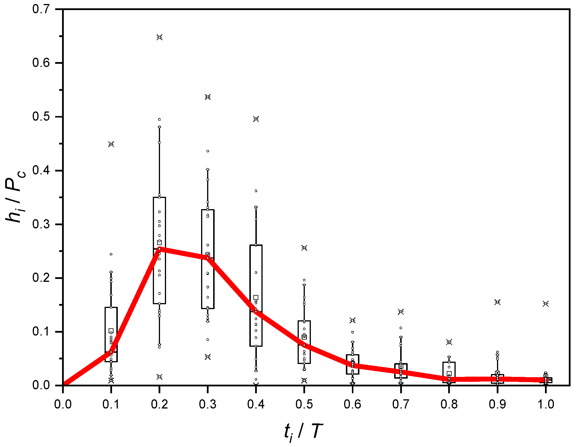
A dimensionless “reference” hyetograph was prepared for the selected 25 precipitation (Figure 10).
In Figure 10, the ranges of changes in measured relative interval values (Δt = 0.1T) of the precipitation amount (hi/Pc) are depicted using box charts that include the pictogram information on the location, dispersion, and shape of the empirical distribution of the studied size. The shape of the box (its range) is shown by the shape of the graph, covering the entire range of data (from the lowest to the highest value). The length of the box is equal to the quarter (quartile) range, i.e., the difference between the first and third quartiles. The quartile is, therefore, one of the measures of the location of given observation values. The first quartile (bottom edge of the box) contains 25% of observations. The second quartile divides the observation collection in half, which corresponds to the median. The third quartile (upper edge of the box) divides the observation dataset into two parts, respectively, with 75% located below this quartile and 25% located above. In Figure 10, the whiskers are limited to the 10% and 90% percentile of the data set (which are identified in the literature by Bonta [42] and Huff [36,48,49], with confidence intervals at 10% and 90%, respectively).
It should be noted that discrete median values in Figure 10 were determined for interval increments of precipitation in contrast to the median illustrated in Figure 9, where these values were determined on the basis of total mass curves. This leads to some differences in the relative values of the height interval peaks such as the peak value hi/Pc, according to sum curves. It falls from the level of approximately 0.29 to approximately 0.25 by interval increments. There are no differences in the peak location itself: r = 0.2ti/T, i.e., in one-fifth of the duration of rainfall.
As stated earlier, the Euler type II model belongs to the group of reference hyetographs/histograms based on the entire IDF curve. It has a dimensional (h, i, q) and discrete (Δt = const = 5 min) form. The features of mass distribution on dimensionless hyetographs of 25 tested precipitation from the IMGW Jelenia Góra station are similar to the Euler type II model. However, this observation requires confirmation in a detailed quantitative assessment similar to the dimensional histogram shapes of these precipitations. These precipitations will, therefore, be subject to a detailed quantitative analysis of similarity to the Euler type II pattern.
For comparative analyses of the shapes of 25 real (dimensional) precipitation histograms, it was necessary to develop standard Euler type II rainfall—from DDF/IDF curves for this station. The model of maximum precipitation amounts (9) was used to create DDF curves, from which precipitation heights were calculated for t = 5, 10, 15, 20, 25, 30, 40, 45, 60, 75, 90, 120, and 180 min and C = 1, 2, 5, and 10 years. It was necessary for the construction of 28 Euler models for seven durations: T = 30, 45, 60, 75, 90, 120, and 180 min (accepted values T, in terms of real precipitation duration and meeting the criterion of division into three equal parts), and in four frequency classes: C = 1, 2, 5, and 10 years.
For the developed Euler type II precipitation, “reference” mass distributions were determined according to the indicator m3 as the ratio of accumulated precipitation for the time from t = 0 to t = 0.33T to total height over time t = T (according to Formula (5)). Mass distributions by indicator m3 proved to be almost identical, independent of T and C. The average value of the indicator was m3 = 0.714. The “model” differentiation of unevenness in the intensity of Euler’s model rainfall by the ni indicator was also analyzed, as the ratio of the maximum intensity of the rainfall interval (Δt = 5 min) to mean intensity over time T (according to Formula (8)). The results of the calculations are given in Table 3.
In the developed Euler type II standard precipitation for the Jelenia Góra station, unevenness according to the indicator ni varies (from 3.47 to 12.03) in individual durations T = 30–180 min, but independent of precipitation (C) frequency of occurrence. Average indicator value ni = 6.96 (Table 3). The value of the peak position ratio in Euler type II models is, on average, r = 0.285 changes in the range of 0.25 for T = 30 min to 0.32 for T = 180 min, regardless of C.
For comparative purposes, for the initial assessment of mass distribution and unevenness in intensity (i) of real precipitation, three indicators were used: r, m3, and ni. They are dedicated especially to quantitative assessments of the similarity of the shape of real precipitation histograms to the Euler type II standard. For the analyzed precipitation (15 C and 10 F with C ∈ [1.0, > 50] years), characteristic (real—referred to time T) values of indicators are: r ∈ [0.07, 0.39], mean value: 0.22, m3 ∈ [0.30, 0.96], mean value: 0.65, ni ∈ [2.16, 9.49], mean value: 4.92.
For comparative purposes of real precipitation histograms with Euler type II model histograms, it was necessary to use a different methodology for interpreting the duration parameter (T) of actual precipitation. Namely, to maintain the principle of creating the Euler model rainfall, i.e., meeting the divisibility of the duration of precipitation into three equal parts, and, at the same time, its divisibility into intervals (with a time step) Δt = 5 min. The actual duration (T) of the rainfall had to be corrected up to their model duration (T’). At stake here is only its correction up (elongation) so as not to lose the mass (height) of actual precipitation. For example, precipitation (of 7 November 2008, with the parameters: Pc = 14.8 mm, T = 38 min, and C = 1.7 years) requires an extension of the actual duration T = 38 min to model one T’ = 45 min. Then penultimate interval Δt, between the 35th and 40th minute, it will contain precipitation from the last 3 min, while the last interval Δt between 40 and 45 min will be empty. On this basis, a re-comparative analysis of real precipitation histograms with Euler’s model histograms was performed for model time T’. Three indicators were again used for quantitative analyzes: r, m3, and ni and were interpreted. For example, r’—as the ratio of the position of the interval Δt = 5 min with the peak cut off (tpeak) maximum height hmax(Δt)—until model time T’ (instead of to time T as in Formula (1)). Similarly, the definitions of other indicators were modified. Characteristic for the model time for the analyzed precipitation T’ indicator values are: r’ ∈ [0.06, 0.38], mean value: 0.21, m3′ ∈ [0.36, 0.97], mean value: 0.69, ni′ ∈ [2.22, 9.51], mean value: 5.23.
The above average values of indicators for model time T’ are slightly lower by 0.01 for r’, while higher by 0.04 for m3′ and 0.31 for ni′, compared to the calculated for the actual duration of precipitation T. However, the results of these analyses allow drawing methodically correct conclusions regarding the comparison of 25 dimensional hyetographs of precipitation from Jelenia Góra with 28 Euler type II models for this station.
- ▪
- Peak position indicator values of maximum height versus time T’, include: r’ ∈ [0.06, 0.38], with an average value r’ = 0.21. The value of this indicator in Euler type II models is on average r = 0.285-changes: r ∈ [0.25, 0.32] for the range T = T’ ∈ [30, 180] min. Both peaks occur in the first, one-third rainfall duration T = T’.
- ▪
- Mass distributions on 25 dimensional histograms were variable within: m3′ ∈ [0.36, 0.97], however average value: m3′ = 0.69 is very close to the constant value m3′ = 0.714 for 28 Euler type II models. In both cases, the main precipitation mass is located in the first, one-third of the duration T = T’.
- ▪
- Rainfall irregularity over 25 histograms was significant within limits ni’∈ [2.22, 9.51], on average ni’ = 5.23 in Euler type II standard precipitation. The unevenness was similar within the limits ni ∈ [3.47, 12.03], on average ni = 6.96. These values should also be considered similar.
4.2.2. DVWK Pattern Verification
For verification of the similarity of shapes of dimensionless hyetographs to the DVWK pattern, frontal and low-pressure precipitation, physically indicated, will be used from the Huff quartile group II (Figure 5). This group shows approximately the specific characteristics of the mass distribution according to the DVWK pattern on a dimensionless hyetograph, where, for the first 30% of the duration of precipitation, 20% of its total amount is present. In the middle of the duration, 70% of the amount appears, and the remaining 30% of the amount occurs in the second half of the duration. Therefore, the DVWK model describes precipitation with the maximum intensity occurring in the middle of the event duration (this distribution is also similar to SCS type II distribution).
A detailed quantitative analysis showing the similarity of dimensionless shapes of hyetographs to the DVWK literature pattern will be subject to 13 precipitations: 10 frontal (T > 180 min) and three low-pressure rainfalls. For comparative purposes, to assess mass distribution and assess unevenness in intensity (i) of real precipitation, seven indicators were used: r, rcg, m1, m2, m4, m5, and ni—dedicated especially to quantitative assessments showing the similarity of the real precipitation hyetographs’ shape to the DVWK pattern. The characteristic values of indicators calculated for the analyzed 13 precipitation rates are: r ∈ [0.05, 0.55], mean value: 0.34, rcg∈ [0.27, 0.49], mean value: 0.38, m1∈ [0.10, 2.29], mean value: 0.92, m2∈ [0.18, 0.46], mean value: 0.31, ni ∈ [1.80, 4.61], mean value: 3.05, m4 ∈ [0.07, 0.61], mean value: 0.37 (median 0.38), m5 ∈ [0.57, 0.93], and mean value: 0.74 (median 0.71).
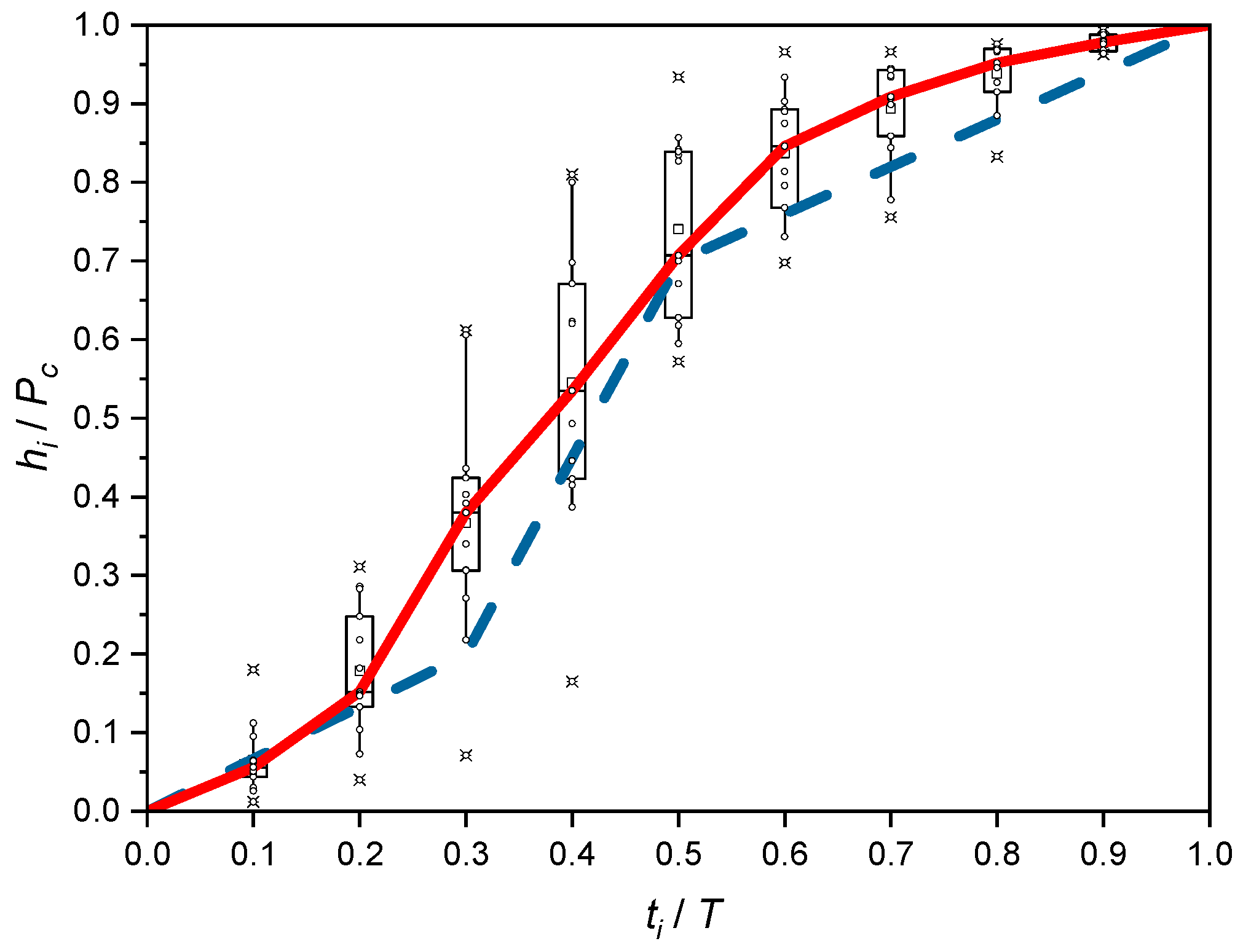
Based on measured and calculated precipitation parameters, a dimensionless ‘standard’ sum curve was developed (from median intervals of dimensionless heights) with the results of measurements in the boxes, shown in Figure 11, along with the polyline curve, according to the DVWK pattern.
The “reference” sum curve represents dimensionless precipitation similar to the DVWK pattern. High compliance of both models occurs for the value of the main indicator m5 mass distribution (i.e., for ti/T = 0.50)—with median value: hi/Pc = 0.71 for the analyzed rainfall and hi/Pc = 0.70 for the DVWK pattern. However, for the mass distribution indicator m4 (for ti/T = 0.30), there are already discrepancies in median values: hi/Pc = 0.38 for the analyzed rainfall and hi/Pc = 0.20 for the DVWK pattern. The average value of unevenness during the intensity of the analyzed precipitation: ni = 3.05 is practically equal to the value ni = 3.00 for the DVWK pattern. For the tested precipitation, according to the course of the sum curve, for the first 20% of the duration (T) will occur in 15% of its total amount (Pc) after a time of 60% T appears as 85% Pc and the remaining 15% Pc will occur at 40% T.
5. Discussion and Conclusions
For IMGW-PIB Jelenia Góra station, based on the maximum precipitation model, time series of maximum rainfall occurrences were determined for the assumed times and frequency of exceedance (C ≥ 1 year, C ≥ 2 years C ≥ 5 years and C ≥ 10 years). To examine the shapes of local hyetographs, precipitation with exceedance frequencies were selected for the statistical analysis C(T) ≥ 1 year, which was then genetically grouped by duration, on precipitation: convective (with T ≤ 120 min), frontal (T ∈ (120, 720] min), and low-pressure (T > 720 min).
To group precipitation due to the similarity of physical–genetic features, various research methodologies were used: Huff, cluster analysis using the Ward method and k-means (for k = 4). These methods, and especially the k-means method, proved to be useful for selecting precipitation in terms of shape hyetographs. Grouping of precipitation by the Huff method does not allow for unambiguous attribution of “standards” to the examined mass hyetographs, depending on the duration of precipitation or the frequency of occurrence. However, it indicates that mass distributions on dimensionless hyetographs of the medians, in the I quartile group is the closest to the Euler type II standard. On the other hand, mass distributions in the II quartile group are similar to the DVWK standard. Grouping of precipitation using the Ward method resulted in the formation of four characteristic clusters of which cluster No. 4 had the distribution of precipitation mass most similar to the Euler type II model. However, the DVWK pattern was not clearly mapped in any of the clusters. For grouping precipitation using the k-means method, the number of clusters was assumed k = 4. More expressive clusters were obtained compared to the results of the Ward clustering. The mass distribution on hyetographs belonging to this cluster is similar to the Euler type II standard, where in one-third of the initial duration of precipitation for approximately two-thirds of its mass and the value of the relative position of the peak is r ≈ (0.2 ÷ 0.3). Precipitation belonging to cluster No. 4 (7% of the population) have intensity increase peaks located in the first, one-fifth part of the duration, more precisely r ≈ 0.2. In addition, this cluster is characterized by the largest numerical value of the height interval peak (almost six times greater than the average), which makes it similar in this respect to the Euler precipitation.
Statistical analysis of the similarity of dimensionless shapes of hyetographs was performed within the separated genetic clusters, with the determination of mass distribution parameters and unevenness in time, defined by eight indicators in the paper. Comparative analysis of test results included verification of the shapes of Euler type II and DVWK standards. For verification of the Euler type II model, convective and frontal precipitation with duration times up to 180 minutes were selected, from clusters No. 3 and 4 obtained by the k-means method. As a result of comparisons, it was found that the mass distribution on 25 dimensional histograms, according to the average value indicator, m3′ = 0.69 is very close to the constant value m3 = 0.71—for 28 Euler type II models. This means that the main rainfall mass is located in the first one-third of the duration T = T’. The value of the peak height indicator of the maximum height hmax(Δt) was, on average, r’ = 0.21, and, in Euler type II models, r = 0.285. Therefore, both peaks occur in the first, one-third rainfall duration T = T’. Generally, it should be stated that the Euler type II standard is suitable for the description of precipitation from the IMGW-PIB mountain station in Jelenia Góra. The tested discrepancies fall within the accuracy class of hydrological measurements and calculations related to random phenomena.
Because the results of cluster analyses did not clearly indicate the specific features of mass distribution according to the DVWK pattern, but only the grouping of precipitation by the Huff method, precipitation verification from the II quartile group was adopted for verification of the pattern, where there are 13 frontal and low rainfall with such characteristics. High compliance of both models was observed for the value of the main mass distribution index m5 where median values: hi/Pc = 0.71 for the analyzed precipitation and hi/Pc = 0.70 for the DVWK pattern. For the second indicator m4, there are already some discrepancies in median values: hi/Pc = 0.38—for the analyzed precipitation and hi/Pc = 0.20 for the DVWK pattern. The distribution of mass of precipitation in Jelenia Góra is as follows: for 20% T—15% Pc, for 60% T—85% Pc (remaining 15% Pc—in 40% T). The average value of unevenness during the intensity of the tested precipitation: ni = 3.05 is practically equal: ni = 3.00—for the DVWK standard. Generally speaking, it should be stated that the DVWK standard is approximate in the class of the accuracy of measurements and hydrological calculations of random phenomena.
The conducted studies allow formulating the following conclusions of practical significance.
- ▪
- Euler type II and DVWK model rainfall patterns are similar to real precipitation (in the case of the analyzed station), so they can be used for hydrodynamic modeling of stormwater drainage.
- ▪
- Development of model rainfall scenarios for hydrodynamic modeling should be based on local DDF/IDF curves (developed for a given location, based on many years of measurements).
- ▪
- In order to obtain reliable hydrodynamic modeling results, both Euler type II and DVWK model rainfall should be used in parallel with real precipitation models. This approach will increase the number of variants and, thus, the certainty of simulations.
The research, according to the methodology proposed in the work, should be continued for more meteorological stations to be confirmed in other regions of Poland.
Author Contributions
Conceptualization, K.W., B.K., M.N. and A.K.; methodology, K.W., B.K., M.N. and A.K.; formal analysis, A.K.; investigation, K.W.; resources, B.K.; writing—original draft preparation, K.W., B.K., M.N. and A.K; writing—review and editing, K.W. and B.K.; visualization, K.W. and B.K.; supervision, A.K.; funding acquisition, B.K. All authors have read and agreed to the published version of the manuscript.
Funding
This research has been carried out as part of the statutory activity of the Faculty of Environmental Engineering at Wroclaw University of Science and Technology, funded by the Ministry of Science and Higher.
Conflicts of Interest
The authors declare no conflict of interest.
References
- Starzec, M. A critical evaluation of the methods for the determination of required volumes for detention tank. E3S Web Conf. 2018, 45, 00088. [Google Scholar] [CrossRef] [Green Version]
- Polish Standard PN-EN 752. Drain and Sewer Systems Outside Buildings—Sewer System Management; PKN: Warsaw, Poland, 2017. [Google Scholar]
- Hänsel, S.; Petzold, S.; Matschullat, J. Precipitation Trend Analysis for Central Eastern Germany 1851–2006. Bioclimatol. Nat. Hazards 2009, 14, 29–38. [Google Scholar] [CrossRef]
- IPCC. Climate Change 2014: Impacts, Adaptation, and Vulnerability (Part A: Global and Sectoral Aspects). Contribution of Working Group II to the Fifth Assessment Report of the Intergovernmental Panel on Climate Change; Field, C.B., Mach, K.J., Mastrandrea, M.D., Eds.; Cambridge University Press: New York, NY, USA, 2014. [Google Scholar]
- Kaźmierczak, B.; Kotowski, A. The influence of precipitation intensity growth on the urban drainage systems designing. Theor. Appl. Climatol. 2014, 118, 285–296. [Google Scholar] [CrossRef]
- Onof, C.; Arnbjerg-Nielsen, K. Quantification of anticipated future changes in high resolution design rainfall for urban areas. Atmos. Res. 2009, 92, 350–363. [Google Scholar] [CrossRef]
- Staufer, P.; Leckebusch, G.; Pinnekamp, J. Die Ermittlung der relevanten Niederschlagscharakteristik für die Siedlungsentwässerung im Klimawandel. KA Korresp. Abwasser Abfall 2010, 57, 1203–1208. [Google Scholar] [CrossRef]
- Arbeitsblatt DWA-A118. Hydraulische Bemessung und Nachweis von Entwässerungssystemen; DWA: Hennef, Germany, 2006. [Google Scholar]
- Schmitt, T.G. Kommentar zum Arbeitsblatt A 118 “Hydraulische Bemessung und Nachweis von Entwässerungssystemen”; DWA: Hennef, Germany, 2000. [Google Scholar]
- Schmitt, T.G.; Thomas, M. Rechnerischer Nachweis der Überstauhäufigkeit auf der Basis von Modellregen und Starkregenserien. KA Wasserwirtsch. Abwasser Abfall 2000, 47, 63–69. [Google Scholar]
- Bruni, G.; Reinoso, R.; Van de Giesen, N.C.; Clemens, F.H.L.R.; Ten Veldhuis, J.A.E. On the sensitivity of urban hydrodynamic modeling to rainfall spatial and temporal resolution. Hydrol. Earth Syst. Sci. 2015, 19, 691–709. [Google Scholar] [CrossRef] [Green Version]
- Kotowski, A. Podstawy Bezpiecznego Wymiarowania Odwodnień Terenów. Sieci Kanalizacyjne (vol. I); Obiekty specjalne (vol. II), 2nd ed.; Seidel-Przywecki: Warsaw, Poland, 2015. [Google Scholar]
- Zawilski, M.; Brzezińska, A. Spatial rainfall intensity distribution over an urban area and its effect on a combined sewerage system. Urban Water J. 2014, 11, 532–542. [Google Scholar] [CrossRef]
- Wartalska, K.; Nowakowska, M.W.; Kaźmierczak, B. Verification of storm water reservoirs operation in hydrodynamic modeling. In Proceedings of the 9th IWA Eastern European Young Water Professionals Conference, Budapest, Hungary, 24–27 May 2017; Feierabend, M., Novytska, O., Bakos, V., Eds.; IWA Publishing: Budapest, Hungary, 2017; pp. 526–533. [Google Scholar]
- Al-Saadi, R. Hyetograph Estimation for the State of Texas. Master’s Thesis, Texas Tech University, Lubbock, TX, USA, December 2002. [Google Scholar]
- DVWK. Arbeitsanleitung zur Anwendung Niederschlag-Abflub-Modellen in kleinen Einzugsgebieten. Regeln 113 (Teil II: Synthese); Verlag Paul Parey: Hamburg, Germany, 1984. [Google Scholar]
- Kotowski, A.; Nowakowska, M. Standards for the dimensioning and assessment of reliable operations of area drainage systems under conditions of climate change. Tech. Trans. Environ. Eng. 2018, 1, 125–139. [Google Scholar] [CrossRef]
- Cronshey, R. Urban Hydrology for Small Watersheds; US Department of Agriculture, Soil Conservation Service, Engineering Division: Washington, DC, USA, 1986.
- Neale, C.M.; Tay, C.C.; Herrmann, G.R.; Cleveland, T.G. TXHYETO. XLS: A Tool to Facilitate Use of Texas-Specific Hyetographs for Design Storm Modeling. In Proceedings of the World Environmental and Water Resources Congress, Austin, TX, USA, 17–21 May 2015; pp. 241–254. [Google Scholar] [CrossRef]
- Chow, V.T.; Maidment, D.R.; Mays, L.W. Applied Hydrology; McGraw-Hill: New York, NY, USA, 1988. [Google Scholar]
- Lin, G.F.; Chen, L.H.; Kao, S.C. Development of regional design hyetographs. Hydrol. Process. 2005, 19, 937–946. [Google Scholar] [CrossRef] [Green Version]
- Veneziano, D.; Villani, P. Best linear unbiased design hyetograph. Water Resour. Res. 1999, 35, 2725–2738. [Google Scholar] [CrossRef]
- Cazanescu, S.; Cazanescu, R.A. New hydrological approach for environmental protection and floods management. Bull. UASVM Agric. 2009, 66, 63–70. [Google Scholar]
- Rivard, G. Design storm events for urban drainage based on historical rainfall data: A conceptual framework for a logical approach. Adv. Mod. Manag. Stormw. 1996, R191–12, 187–199. [Google Scholar] [CrossRef] [Green Version]
- Yen, B.C.; Chow, V.T. Design hyetographs for small drainage structures. J. Hydraul. Eng. Div. ASCE 1980, 106, 1055–1976. [Google Scholar]
- Griffiths, G.A.; Pearson, C.P. Distribution of high intensity rainfalls in metropolitan Christchurch, New Zealand. J. Hydrol. 1993, 31, 5–22. Available online: https://www.jstor.org/stable/43944695 (accessed on 30 September 2019).
- Ellouze, M.; Abida, H.; Safi, R. A triangular model for the generation of synthetic hyetographs. Hydrol. Sci. J. 2009, 54, 287–299. [Google Scholar] [CrossRef]
- Sifalda, V. Entwicklung eines Berechnungsregens für die Bemessung von Kanalnetzen. GWF Wasser Abwasser 1973, 114, 435–440. [Google Scholar]
- Desbordes, M. Urban runoff and design storm modeling. In Proceedings of the First International Conference on Urban Drainage, London, UK, April 1978; pp. 353–361. [Google Scholar]
- Lee, K.T.; Ho, J.Y. Design hyetograph for typhoon rainstorms in Taiwan. J. Hydrol. Eng. 2008, 13, 647–651. [Google Scholar] [CrossRef]
- Peyron, N.; Nguyen, V.T.V.; Rivard, G. An optimal design storm pattern for urban runoff estimation in southern Québec. In Proceedings of the 30th Annual Conference of the Canadian Society for Civil Engineering, Montréal, QC, Canada, 5–8 June 2002. [Google Scholar]
- Keifer, C.J.; Chu, H.H. Synthetic storm pattern for drainage design. J. Hydr. Eng. Div. 1957, 83, 1–25. [Google Scholar]
- Kaźmierczak, B.; Kotowski, A. Weryfikacja Przepustowości Kanalizacji Deszczowej w Modelowaniu Hydrodynamicznym; Oficyna Wyd. Politechniki Wrocławskiej: Wroclaw, Poland, 2012. [Google Scholar]
- Kotowski, A.; Kaźmierczak, B.; Nowakowska, M. Analiza obciążenia systemu odwodnienia terenu w przypadku prognozowanego zwiększenia częstości i intensywności deszczów z powodu zmian klimatycznych. Ochr. Sr. 2013, 35, 25–32. [Google Scholar]
- Kotowski, A.; Kaźmierczak, B.; Dancewicz, A. Modelowanie Opadów do Wymiarowania Kanalizacji; KILiW PAN (IPPT): Warsaw, Poland, 2010. [Google Scholar]
- Huff, F.A. Time distribution of rainfall in heavy storms. Water Resour. Res. 1967, 3, 1007–1019. [Google Scholar] [CrossRef]
- Bonta, J.V.; Rao, A.R. Factors affecting development of Huff curves. Trans. ASAE 1987, 30, 1689–1693. [Google Scholar] [CrossRef]
- Pani, E.A.; Haragan, D.R. A comparison of Texas and Illinois temporal rainfall distributions. In Proceedings of the Fourth Conference on Hydrometeorology, Reno, NV, USA, 7–9 October 1981; American Meteorological Society: Boston, MA, USA, 1981; pp. 76–80. [Google Scholar]
- Terranova, O.G.; Iaquinta, P. Temporal properties of rainfall events in Calabria (southern Italy). Nat. Hazard. Earth Syst 2011, 11, 751–757. [Google Scholar] [CrossRef] [Green Version]
- Elfeki, A.M.; Ewea, H.A.; Al-Amri, N.S. Development of storm hyetographs for flood forecasting in the Kingdom of Saudi Arabia. Arab. J. Geosci. 2014, 7, 4387–4398. [Google Scholar] [CrossRef]
- Pan, C.; Wang, X.; Liu, L.; Huang, H.; Wang, D. Improvement to the Huff Curve for Design Storms and Urban Flooding Simulations in Guangzhou, China. Water 2017, 9, 411. [Google Scholar] [CrossRef] [Green Version]
- Bonta, J.V. Development and utility of Huff curves for disaggregating precipitation amounts. Appl. Eng. Agric. 2004, 20, 641–652. [Google Scholar] [CrossRef]
- Awadallah, A.G.; Elsayed, A.Y.; Abdelbaky, A.M. Development of design storm hyetographs in hyper-arid and arid regions: Case study of Sultanate of Oman. Arab. J. Geosci. 2017, 10, 456. [Google Scholar] [CrossRef]
- Banasik, K.; Wałęga, A.; Węglarczyk, S.; Więzik, B. Aktualizacja Metodyki Obliczania Przepływów i Opadów Maksymalnych o Określonym Prawdopodobieństwie Przewyższenia dla Zlewni Kontrolowanych i Niekontrolowanych oraz Identyfikacji Modeli Transformacji Opadu w Odpływ; KZGW: Warsaw, Poland, 2017.
- Powell, D.N.; Khan, A.A.; Aziz, N.M.; Raiford, J.P. Dimensionless rainfall patterns for South Carolina. J. Hydrol. Eng. 2007, 12, 130–133. [Google Scholar] [CrossRef]
- Vandenberghe, S.; Verhoest, N.; Buyse, E.; De Baets, B. A stochastic design rainfall generator based on copulas and mass curves. Hydrol. Earth Syst. Sci. 2010, 14, 2429–2442. [Google Scholar] [CrossRef] [Green Version]
- Licznar, P.; Szeląg, B. Analiza zmienności czasowej opadów atmosferycznych w Warszawie. Ochr. Sr. 2014, 36, 23–28. [Google Scholar]
- Huff, F.A. Time Distributions of Heavy Rainstorms in Illinois; Circular. Illinois State Water Survey 173: Champaign, IL, USA, 1990; Available online: http://hdl.handle.net/2142/94492 (accessed on 30 September 2019).
- Huff, F.A.; Angel, J.R. Rainfall Frequency Atlas of the Midwest; Illinois State Water Survey 71: Champaign, IL, USA, 1992; Available online: http://hdl.handle.net/2142/94532 (accessed on 30 September 2019).
- Banasik, K.; Bodziony, M.; Bogdanowicz, E.; Chormański, J.; Górski, D.; Jaworski, W.; Madzia, M.; Marcinkowski, M.; Niedbała, J.; Olearczyk, D.; et al. Metodyka Obliczania Przepływów i Opadów Maksymalnych o Określonym Prawdopodobieństwie Przewyższenia dla Zlewni Kontrolowanych i Niekontrolowanych oraz Identyfikacji Modeli Transformacji Opadu w Odpływ; KZGW: Warsaw, Poland, 2009.
- Wierzchoń, S.; Kłopotek, M. Algorytmy Analizy Skupień; WNT: Warsaw, Poland, 2015. [Google Scholar]
Figure 1.
Typical rainfall intensity distributions over time, according to DVWK [16]: (a) constant intensity precipitation (i.e., block precipitation), (b) precipitation with a maximum intensity at the beginning, (c) precipitation with a maximum intensity at the center, and (d) precipitation with maximum intensity at the end.

Figure 2.
Diagram of Euler type II model precipitation [12].
Figure 2.
Diagram of Euler type II model precipitation [12].

Figure 3.
Recommended distribution of rainfall sums according to DVWK [44].
Figure 3.
Recommended distribution of rainfall sums according to DVWK [44].

Figure 4.
Location of the IMGW-PIB Jelenia Góra measuring station.

Figure 5.
Dimensionless rainfall curves with a median curve for 4 Huff quartile groups: (a) I quartile, (b) II quartile, (c) III quartile, and (d) IV quartile.
Figure 5.
Dimensionless rainfall curves with a median curve for 4 Huff quartile groups: (a) I quartile, (b) II quartile, (c) III quartile, and (d) IV quartile.

Figure 6.
Dendrogram of precipitation grouping using the Ward method.

Figure 7.
Dimensionless precipitation mass curves with a median for four clusters according to the Ward method: (a) Cluster No. 1, (b) cluster No. 2, (c) cluster No. 3, and (d) cluster No. 4.
Figure 7.
Dimensionless precipitation mass curves with a median for four clusters according to the Ward method: (a) Cluster No. 1, (b) cluster No. 2, (c) cluster No. 3, and (d) cluster No. 4.

Figure 8.
Dimensionless rainfall mass curves with a median for four clusters separated by the k-means method: (a) Cluster No. 1, (b) cluster No. 2, (c) cluster No. 3, and (d) cluster No. 4.
Figure 8.
Dimensionless rainfall mass curves with a median for four clusters separated by the k-means method: (a) Cluster No. 1, (b) cluster No. 2, (c) cluster No. 3, and (d) cluster No. 4.

Figure 9.
Dimensionless mass curves with a median for 15 convective (C) and 10 frontal (F with T ≤ 180 min) rainfall from clusters No. 3 and 4 (for k = 4).
Figure 9.
Dimensionless mass curves with a median for 15 convective (C) and 10 frontal (F with T ≤ 180 min) rainfall from clusters No. 3 and 4 (for k = 4).

Figure 10.
Dimensionless “reference” hyetograph for 25 precipitation (with T ≤ 180 min) with box charts with measurement results.
Figure 10.
Dimensionless “reference” hyetograph for 25 precipitation (with T ≤ 180 min) with box charts with measurement results.

Figure 11.
Box plot hyetograph of 10 frontal and three low-pressure precipitation (solid line) together with the DVWK pattern (dashed line).
Figure 11.
Box plot hyetograph of 10 frontal and three low-pressure precipitation (solid line) together with the DVWK pattern (dashed line).


Table 1.
Number of precipitations in separate time groups and exceedance classes.
| Classification | Number of Rainfall (Percent) | ||||
|---|---|---|---|---|---|
| Duration | t ≤ 120 min | ≤60 min | 10 (12%) | 23 (29%) | 80 (100%) |
| (60, 120] min | 13 (16%) | ||||
| t ∈ (120, 720] min | (120, 180] min | 13 (16%) | 39 (49%) | ||
| (180, 360] min | 12 (15%) | ||||
| (360, 720] min | 14 (18%) | ||||
| t > 720 min | (720, 1440] min | 11 (14%) | 18 (22%) | ||
| >1440 min | 7 (9%) | ||||
| Frequency of Occurrence | C ∈ [1, 2) years | 26 (33%) | 80 (100%) | ||
| C ∈ [2, 5) years | 24 (30%) | ||||
| C ∈ [5, 10) years | 9 (11%) | ||||
| C ≥ 10 years | 21 (26%) | ||||
Table 2.
Number of precipitations by exceedance frequency classes in Huff’s quartile groups.
| Exceedance Classes C | Quartile Groups | Total | |||
|---|---|---|---|---|---|
| I | II | III | IV | ||
| C ∈ [1, 2) years | 14 | 5 | 5 | 2 | 26 (33%) |
| C ∈ [2, 5) years | 8 | 10 | 5 | 1 | 24 (30%) |
| C ∈ [5, 10) years | 4 | 2 | 2 | 1 | 9 (11%) |
| C ≥ 10 years | 4 | 10 | 7 | 0 | 21 (26%) |
| Total | 30 (37%) | 27 (34%) | 19 (24%) | 4 (5%) | 80 (100%) |
Table 3.
The values of the ni indicator for Euler type II models.
| Frequency of Rainfall Occurrence | Rainfall Duration T, Min | Mean | ||||||
|---|---|---|---|---|---|---|---|---|
| 30 | 45 | 60 | 75 | 90 | 120 | 180 | ||
| C = 1 year | 3.47 | 4.60 | 5.60 | 6.56 | 7.43 | 9.10 | 12.05 | 6.97 |
| C = 2 years | 3.46 | 4.59 | 5.61 | 6.53 | 7.44 | 9.05 | 11.99 | 6.95 |
| C = 5 years | 3.47 | 4.59 | 5.61 | 6.55 | 7.43 | 9.06 | 12.04 | 6.96 |
| C = 10 years | 3.47 | 4.60 | 5.61 | 6.55 | 7.44 | 9.07 | 12.02 | 6.97 |
| Mean | 3.47 | 4.60 | 5.61 | 6.55 | 7.43 | 9.07 | 12.03 | 6.96 |
© 2020 by the authors. Licensee MDPI, Basel, Switzerland. This article is an open access article distributed under the terms and conditions of the Creative Commons Attribution (CC BY) license (http://creativecommons.org/licenses/by/4.0/).
Share and Cite
MDPI and ACS Style
Wartalska, K.; Kaźmierczak, B.; Nowakowska, M.; Kotowski, A. Analysis of Hyetographs for Drainage System Modeling. Water 2020, 12, 149. https://doi.org/10.3390/w12010149
AMA Style
Wartalska K, Kaźmierczak B, Nowakowska M, Kotowski A. Analysis of Hyetographs for Drainage System Modeling. Water. 2020; 12(1):149. https://doi.org/10.3390/w12010149
Chicago/Turabian StyleWartalska, Katarzyna, Bartosz Kaźmierczak, Monika Nowakowska, and Andrzej Kotowski. 2020. "Analysis of Hyetographs for Drainage System Modeling" Water 12, no. 1: 149. https://doi.org/10.3390/w12010149
Note that from the first issue of 2016, this journal uses article numbers instead of page numbers. See further details here.