Pump Efficiency Analysis for Proper Energy Assessment in Optimization of Water Supply Systems


Departamento de Ingeniería Civil, Hidráulica, Energía y Medio Ambiente, Universidad Politécnica de Madrid, 28040 Madrid, Spain
*
Author to whom correspondence should be addressed.
Water 2020, 12(1), 132; https://doi.org/10.3390/w12010132
Submission received: 29 November 2019
/
Revised: 17 December 2019
/
Accepted: 24 December 2019
/
Published: 31 December 2019
(This article belongs to the Special Issue Water Resources Management Models for Policy Assessment)
Abstract
:Water supply systems need to be designed accounting for both construction and operational costs. When the installation requires water pumping, it is key for the operational costs to know how well the pump can perform. So far, pump efficiency has been considered using conservative values, in the absence of a better estimation. The aim of this paper was to improve determining the energy costs by clarifying what the value of the pump performance should be. For this, 226 commercial pumps were studied, registering the efficiency at the optimum operating point, as well as other variables such as the flow rate, height, and pump type. As a result, a strong relationship between the pump performance and the discharge flow was spotted. That allowed the generation of an empirical curve, which can be used by designers to anticipate what pump efficiency can be expected. The results are used in a simple case study using the Granados Optimization System. These achievements can be implemented in design policies for a better energy assessment in the optimization of water supply systems.
1. Introduction
Under the climate change threat, becoming energetically efficient is now a crucial necessity for our society. A proper energy assessment is, therefore, a key factor to account for in the developing of new policies that look after sustainable designs of water supply systems [1]. The designing stage of a water distribution system requires considering not only the construction phase, but also the operation of the facility over its entire lifespan. With this approach, energy expenditure takes a huge fraction of the final cost, and it should not be dismissed from the calculations. There are many designing approaches that do incorporate this aspect in their analysis. Mala-Jetmarova et al. [2] summarized what other authors considered in their proposals. After their review of the state of art, it seems that the design of water distribution systems is increasingly emphasizing the importance of including operation assessments.
The operational costs are often included in optimization algorithms in a single economic function that would also include construction costs of the network. This approach is used in some classical studies, like [3], but it is still the most common way to assess energy costs in the design. That is the case of [4,5,6,7,8,9] or [10]. Nevertheless, a different perspective is to treat operational and construction costs as separated objectives, as [11] does. However, this assessment confirmed that such a perspective throws back very different design solutions: the optimum design for construction costs means the highest operational investment and vice versa. This approach makes the search of the optimum for the overall installation more difficult, and therefore it is more advisable to adopt a single cost function to optimize.
In order to achieve a more precise assessment of all costs involved, multiobjective algorithms have started to incorporate in the optimization function costs of maintenance [12,13], replacement [14,15,16], and greenhouse gas emissions [17,18,19,20], among others. Multiobjective methods offer a very complete revision of all costs, but many times they require complex programming, resulting in being computationally expensive and hard to use. The work of [21] explained the state of the art of the multiobjective techniques.
Because operation costs are distributed along the lifespan of the installation, they need to be computed at the design stage. The equivalence is calculated using an accumulative factor that depends on the duration of the operation of the water drive considered, the duration of the construction period, and the discount rate employed. Regarding the lifespan of the facility, some methodologies consider an operative life of 20 years [3,5], but other authors [15,16,20] prefer to carry out the analysis for 100 years.
Another key variable for the operation costs is the pump efficiency. One of the most widely used methods for designing water supply systems in Spain is the Granados System [22,23], which is a gradient-based procedure. Among all variables affecting the Granados System, the pump efficiency is the key factor for calculating the diameter of the hydraulic conduction. The aim of this paper is to define the relationship between the pump’s efficiency and the other parameters involved in the procedure, such as the flow rate, the pumping head and the required power. This pump efficiency analysis does not only serve for the purposes of the Granados System, but it can also help in many other methods that require the value of the pump’s efficiency. This is the case of [24], where they use an estimated value of 75% in their calculations; for Wu et al. [15], the values range from 81% to 84%; Gessler and Walski [25] estimate the efficiency as 75% and so do Alperovits and Shamir [26] and Featherstone and El-Jumaily [27].
Other studies have also decided to optimize the design using as key variables the pump location [28,29], pump capacity [4], type [19], power [3], pumping head [30,31,32], pumping schedule [24,33], or pressure [34,35]. Water supply system design is a complex task where many variables are involved [36] and inter-connected; the decision-making needs a full comprehension of how each factor affects the installation. Some of the relationships between variables are still unknown and only intuited by experience. For this purpose, sensitivity analyses are necessary. The work [37] carries out an exhaustive sensitivity analysis using Sobol’s method (a variance-based approach) to determine the variables that most affect the installation. These variables could vary from pipe diameters to tank sizes, and the degree of influence depends on each case study. In their work, they prove the computational savings that can be obtained and, therefore, how beneficial the analysis is. This paper also intends to serve as a sensitivity analysis of how much pump efficiency is influenced by other factors and how the pump’s efficiency can affect the final cost of a water supply system.
Since the pump efficiency can substantially affect the design of water supply systems due to the wide range of values they can adopt, with this study we carry out an extensive study of the pump performance in order to characterize its values. For this to be made, we analyze the features of commercial pumps available in the market. The conclusions are integrated in a gradient-based procedure, using as a base the Granados System, giving rise to an optimized design method that accounts for the construction and operational costs. This procedure is also compatible with adding other variables such as the carbon footprint [38] of the design or the GHG emissions. Our new methodology is applied to a case study to illustrate its computationally straightforward conception.
2. Materials and Methods
2.1. Brief Summary of the Granados System
Granados System is a pipe-sizing method indicated for the design of branched water distribution systems. It is a gradient based methodology. It is, in fact, based on the ‘change gradient’ concept: The change gradient is defined as the cost of reducing one meter of head loss by increasing the pipe diameter from to the next bigger one :
where Pi and Pj are prices of pipes of length L and diameters and , respectively; ∆hiq and ∆hjq are the head losses of a pipe of length L and diameters and , respectively, when a flow rate q is circulating. When the head losses are calculated using Manning’s formulation, the change gradient’s expression is:
with n being Manning’s friction coefficient.
The definition of the change gradient also needs to include some other associated costs such as excavation expenditure or reinforcements against chemically aggressive environment or hydraulic transients. During the optimization stage, hydraulic transients are usually taken into account in a simplified way, for instance, extra thickness of the pipes to withstand water hammer transient pressure. Once the optimum design is achieved, proper assessment of water hammer should be carried out to verify the initial hypothesis. These associated cost factors increase the pipe price, and therefore, they have to be accounted in the design through Pi and Pj.
Increasing the pipe’s diameter means a reduction in the head loss along the pipeline, but it has the extra cost of the wider and more expensive tube. Since the change gradient is the cost of reducing the head loss by one meter, it needs to be compared to the cost of the energy required for pumping the water at one meter height throughout the entire life of the facility, CE1, which reads:
where CaE1 is the annual energy cost per meter, fA is the discount factor, nc is the duration of the construction period, nu is the useful life of the installation, i is the discount rate, V is the annual volume of water to pump, μB and μM are the pump and engine efficiency, and lastly pE is the unit price of energy.
As it is justified in Granados’ work, with the exception of the pump performance μB, the other variables in the previous equation are relatively known data: V is the total demanded volume to pump, pE is the unit price of the energy that has been hired, and fA is calculated from the discount rate i, the service life nU of the water pipeline which depends on the chosen material, and the construction period nC. Regarding the engine efficiency μM, although it varies theoretically depending on the model chosen and the operating point of the pump, the variations in engine performance are so small that it can be considered constant across different models and manufacturers. Therefore, the above equation can be simplified to:
As previously said, Granados System consists of comparing the cost of building a wider pipe (change gradient) and reducing the head loss by a meter, to the cost of pumping one meter of head loss (CE1). The reasoning is the following:
- If < CE1 ⇒Diameter is preferable to .
- If > CE1 ⇒Diameter is preferable to .
But since CE1 depends on the pump efficiency µB, the procedure changes to:
- If .
- If .
This means that, whenever there is a pump on the market whose efficiency can be greater than the calculated µB, the optimum diameter will be . In the event that no commercial pump can reach that performance because it is very high, it will be necessary to move to the next diameter . Therefore, to apply this method it is necessary to know the maximum efficiency that pumps can reach. This is an uncertainty of the Granados System, and up to now, typically, pump efficiency values around 80% are already indicative.
2.2. Methodology
Among all variables affecting Granados System, the pump performance is the key factor for calculating the diameter of the hydraulic conduction. Nevertheless the results may vary significantly depending on the pump efficiency; indeed, µB presents a wide range of possible values that typically goes from 70% up to 90%. This means a variability of almost 20% in the estimation of the cost, which is a substantial difference. Therefore the aim of this paper is to define the relationship between the pump’s performance and the other parameters involved in the procedure, such as the flow rate, the pumping head or the required power. For this to be done, we select 400 commercial pumps from the catalogues of several manufactures. We discard custom-made pumps since the cost of these pumps is much higher than the ordinary ones listed and the offering in commercial catalogues is already very wide. The selected pumps vary from each other in their type, impeller diameter, number of stages, rotation speed (electrical current frequency, number of poles), brand, etc. For all these models, we study the pump efficiency; in particular, we register the optimum value together with the correspondent flow rate, head and power consumed. Nevertheless, some pumps are ruled out of the sample and presentation of the results because they either were similar to those of other manufacturers, or because they were very specific for some industrial or sanitary engineering uses. In the end, the sample consists of 226 hydraulic pumps.
For the detailed study of the pump performance, this research has focused on the most common type of pump for the applications in civil engineering (supply, irrigation, sanitation, etc.)—centrifugal pumps. Within centrifugal pumps, both horizontal and vertical axes are selected, mostly with a radial flow configuration, with the exception of submersible pumps, for which the axial arrangement is more common. The sample includes regular horizontal and vertical pumps, split case pumps, multistage and submersible pumps. The manufacturers used for this analysis were IDEAL, WILO, ESPA and HASA. More specifically, the commercial models were:
- Split case pumps: CP/CPI/CPR series.
- Horizontal pumps (normalized in the European Union): RNI/RN series.
- Multistage horizontal pumps: APM series.
- Vertical pumps: VS/VG series.
- Submersible vertical pumps: SVA/SVH series.
Multistage pumps perform with the same efficiency for a specific flow rate and different heights (which is the number of stages multiplied for the unitary head). To avoid this dispersion that could make it difficult to draw conclusions, it was decided to only use the optimum operating point correspondent to a single stage.
Using the data collected for the optimum operating points for all the 226 hydraulic pumps previously mentioned (pump’s optimum efficiency and associated flow rate, head, speed, power, frequency, diameter, etc.) we carried out an analysis to establish relationships among the design variables of a water drive.
3. Results and Discussion
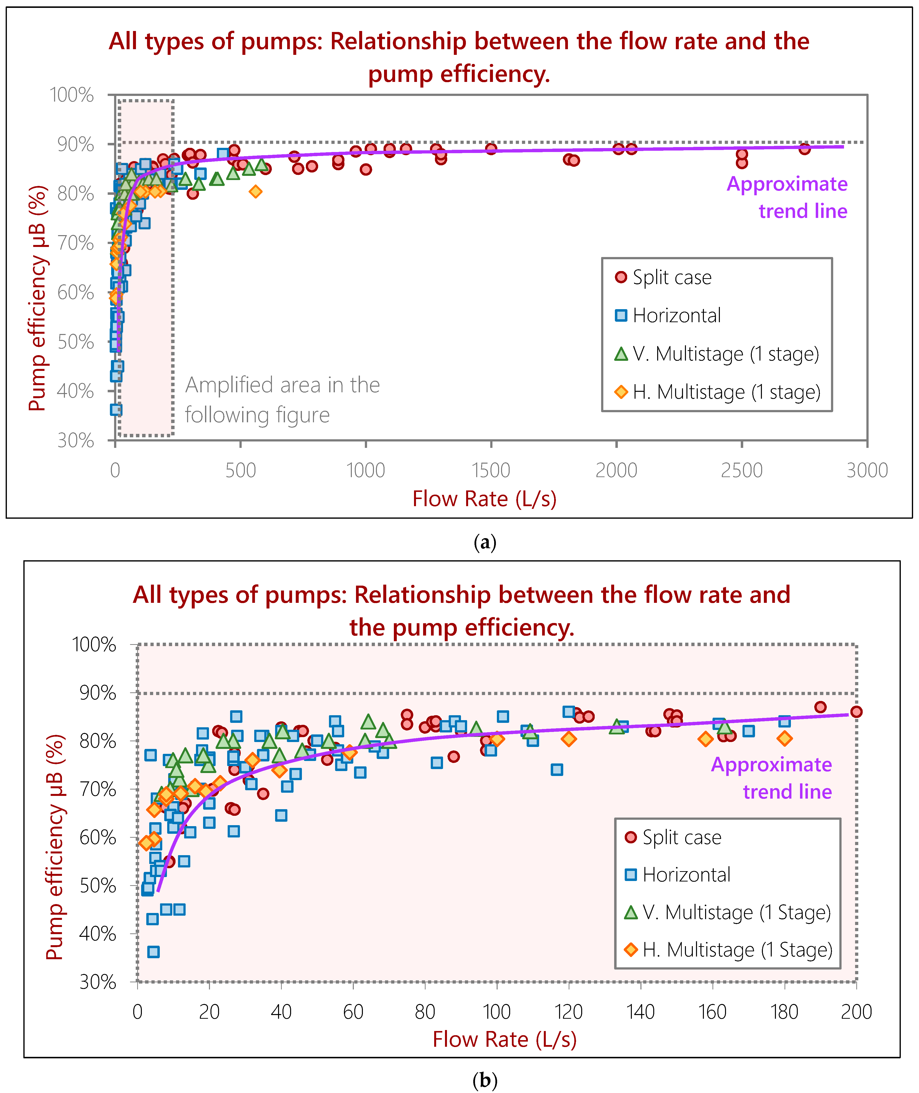
Figure 1a shows the values of the optimum efficiency of the pump and the flow rate correspondent to that point. From it, it can be seen that there is a relationship between both variables: the performance of the pump improves as the discharge increases, although it seems to reach a horizontal asymptote for µB around 90%. In this same figure, it can be spotted that the relationship between the two variables is more precise for flow rate values that are greater than 500 L/s. Below this value, as it can be seen in Figure 1b, there is more dispersion. Also, when the discharge is at least 100 L/s, the pump efficiency can be expected to be better than 80%, but under it, the dispersion is stronger. On the other hand, it has been studied whether the type of pump has any relation with the efficiency. For that, Figure 1 also shows the distribution of the operating points for the split case pumps, horizontal and multistage (both horizontal and vertical).
Regarding the pump type, we conclude that:
- Split case pumps are, in general, the ones that provide the best performance for flow rates over 500 L/s.
- Between 100 L/s and 500 L/s, both split case and horizontal offer the best results.
- Under 100 L/s, the distribution is very heterogeneous and disperse, but as a general rule, there is always a horizontal pump that can provide the best efficiency (but also the lowest, due to the dispersion). Vertical pumps also show great performances, but they can generally be exceeded by a horizontal model.
- Vertical multistage pumps always give a better efficiency than horizontal multistage pumps.
- For small flow rates, the differences between the pump efficiency among models are very high. Different models can almost double other pump’s efficiency, meaning that the energy cost can be almost twice as much if the pump is not well selected. This is why the pump analysis is more complicated for small discharge values.
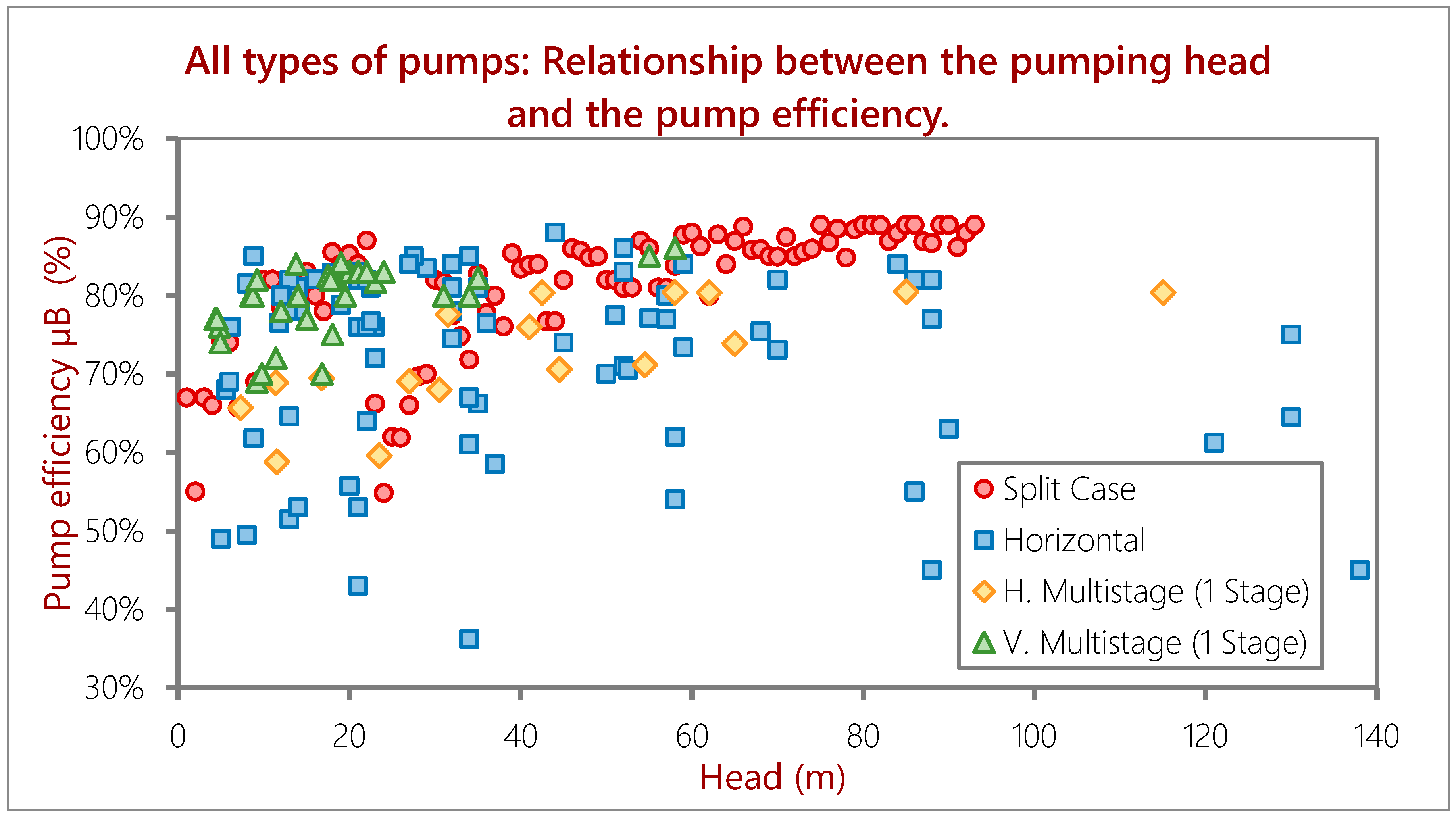
When the pumping height and the efficiency are plotted together, as shown in Figure 2, there is no clear sign of a relationship between the two variables since the dispersion is too strong for any head value. There is a very light tendency of high pump performances (around 80%) for under 40 m head, but over 60 m the distribution of µB is too scattered.
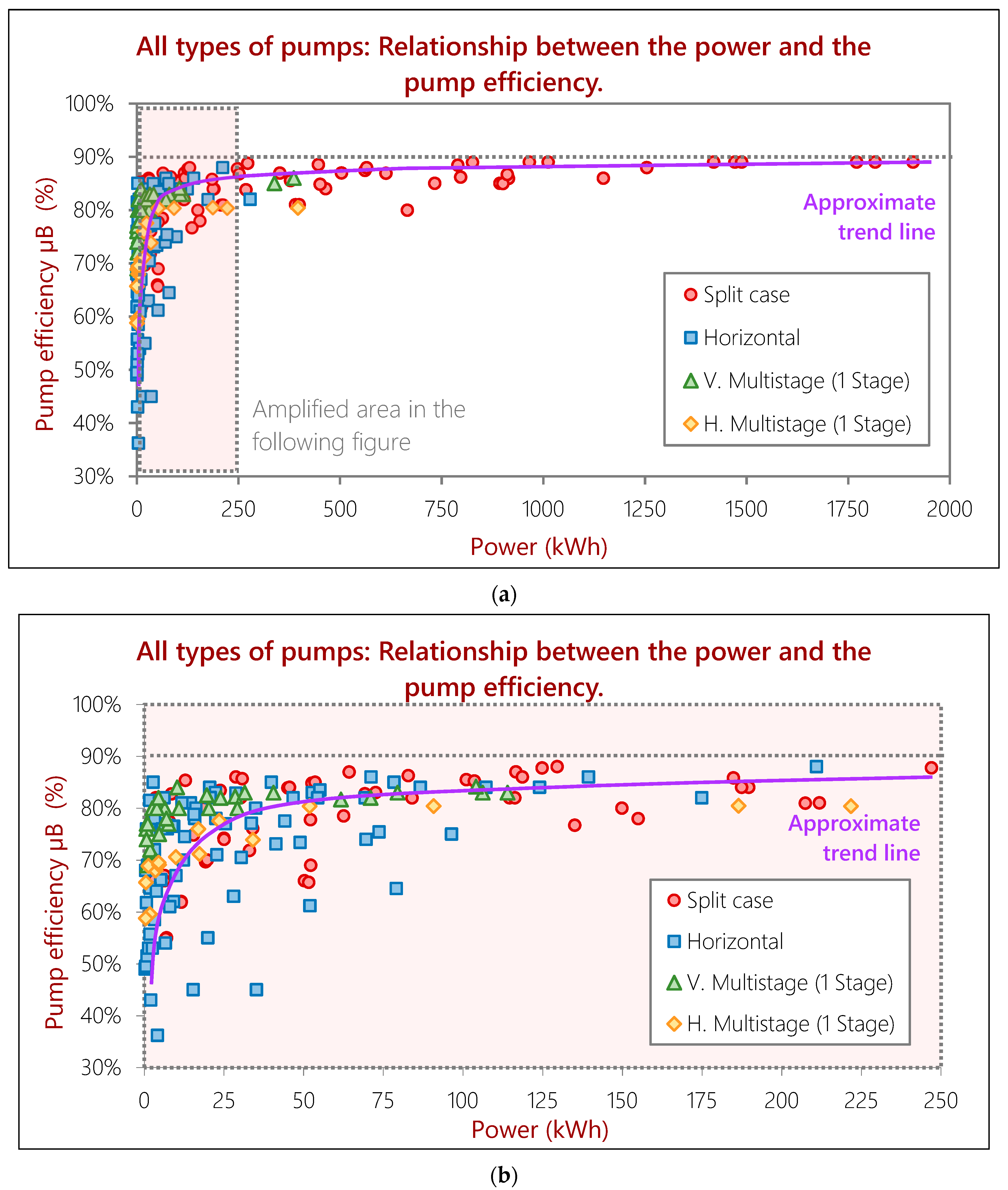
To test out what the relationship between the optimum µB and the required power for that operating point is, Figure 3 was elaborated.
The main conclusions drawn from Figure 3 are:
- There is a relationship between the pump efficiency and the required power for the optimum operating point.
- The relation seems to be clearer from 400 kW and on, and values greater than 80% efficiency can be expected.
- This relationship seems to be weaker than the existing one between the flow rate and the pump efficiency. The interpreted reason for this fact is that, since the power is calculated from the flow rate and the pumping height, the good relationship that the flow rate transfers to the power is weakened by the poor bond that the pumping head and efficiency have. The authors of [3] had already presented similar conclusions. In their work, they empirically proved that the cost of pumping depended on power; which indeed agrees with these results.
To summarize, this first assessment concludes that the strongest of the relationships with the pump efficiency is that of the flow rate, especially when the flow is greater than 100 L/s and it is almost linear.
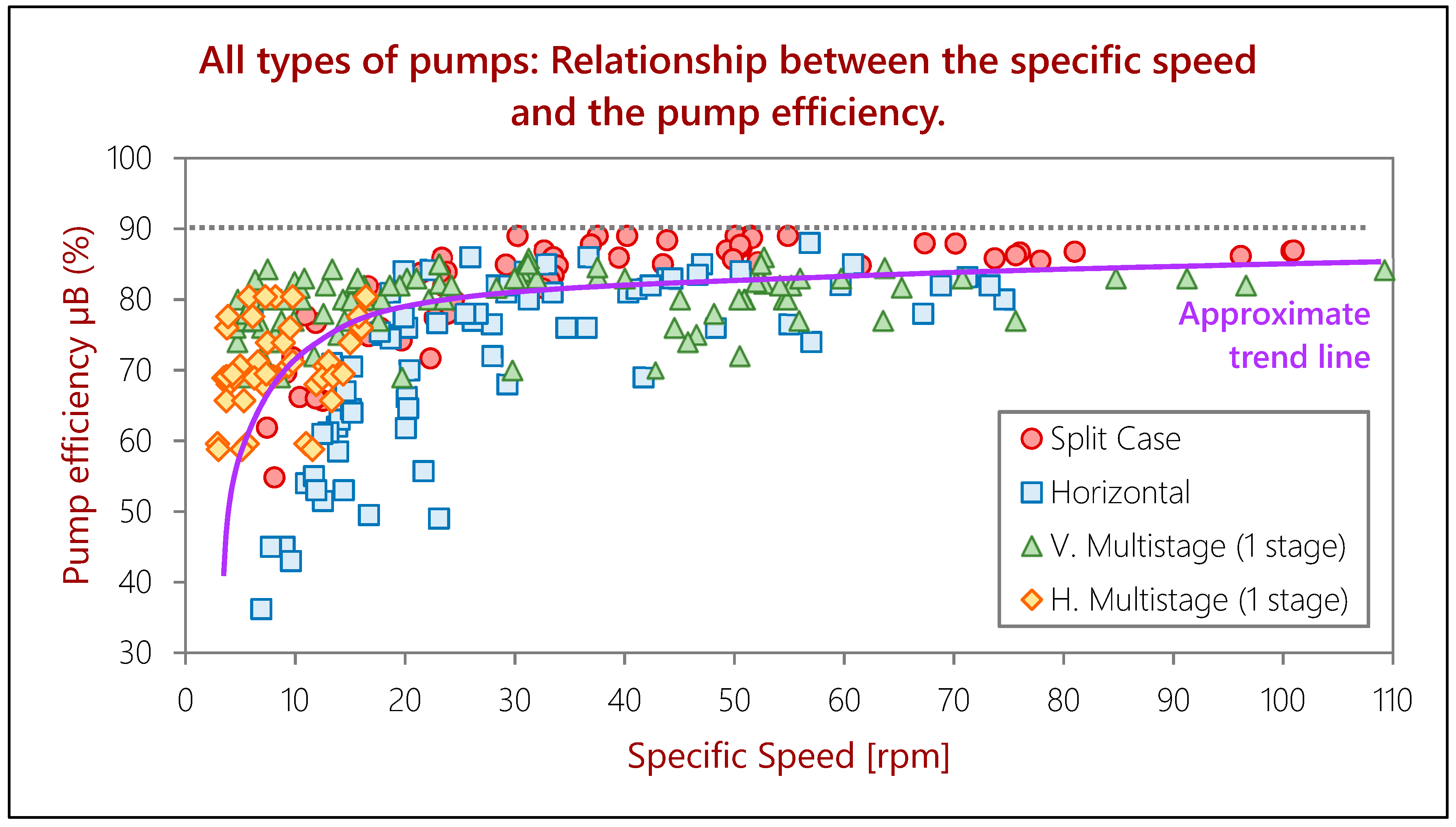
On the other hand, the relationship between the specific speed of the pump and the efficiency is shown in Figure 4. The specific speed of the pump is defined as:
where ns is the specific speed; q, H and nr are the flow rate, pumping head and the rotation speed, respectively, at the optimum operating point [39]. It is interpreted as the rotation speed that a geometrically similar pump should have in order to elevate a discharge of 1 m3/s at 1 m height.
Low specific speed indicates that the pump is suitable for small flow rates and great heights. This means that, since small flow rates have a poorer relationship with the pump efficiency, pumps with a low specific speed will have the worst performance values. This is shown in Figure 4. On the contrary, high specific speed is an indicator of a pump suitable for great flow rates and low heights. According to the previous analysis made from Figure 1, greater discharges correspond to better performances, and therefore, a high specific speed can be associated with a good µB, as Figure 4 shows. The scattering of the figure is caused by the poor relationship that the pumping height and the rotation speed have with the pump efficiency. However there is a diffuse tendency of increasing µB as the specific speed grows. As far as pump type is concerned, the types of pumps that operate at higher flow rates will be the ones with a greater specific speed and therefore, better performance: These are split case pumps, as shown in Figure 4. Vertical multistage pumps also give good results in the smaller flow rate ranges.
3.1. Relationship between the Flow Rate and the Pump Efficiency
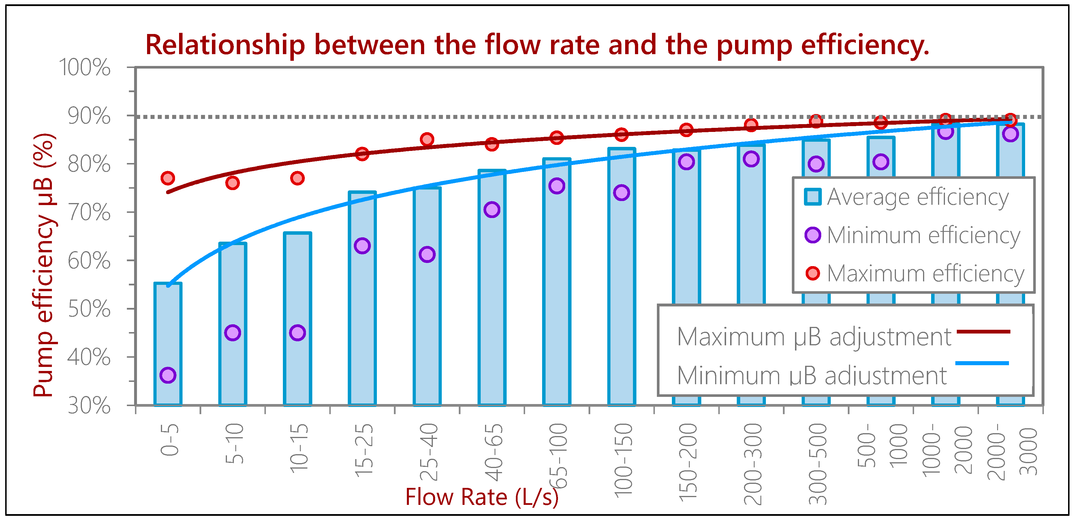
From the previous figures, it seems that there are three flow rate ranges where the relationship with the pump efficiency is different. The first one would be from 0 to 100 L/s, the second from 100 to 500 L/s and the last one over 500 L/s. Nevertheless, in order to be more precise, instead of three zones, the curve has been fitted using up to fourteen flow rate subdivisions. Table 1 shows the average optimum pump efficiency for each interval, as well as the maximum and minimum found among the studied pumps.
When these values are adjusted through a doubly logarithmic curve, the relationships for both the average and maximum values fit satisfactorily (r2 > 98% and r2 > 90%, respectively), as can be seen in Figure 5. The empirical equations that relate the optimum pump efficiency and the flow rate are:
where q is the flow rate in liters per second (L/s).
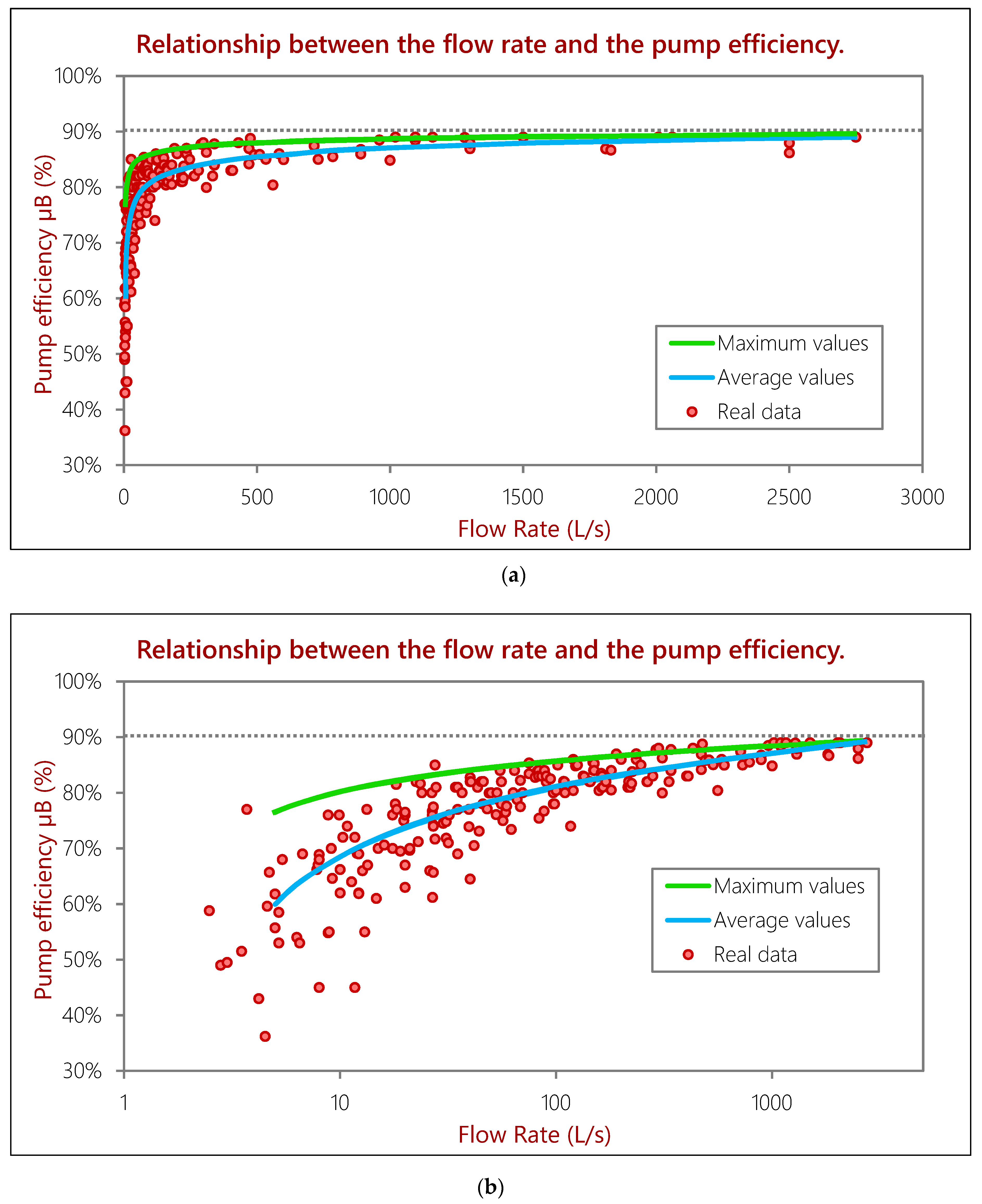
Finally, Figure 6 shows the adjusted curves along with the collected data. Both curves fit satisfactorily for most flow rate ranges, especially for the bigger ones; nevertheless the dispersion is higher for the small discharge values (under 50 L/s), but still, it gives a valid reference. To facilitate the visualization, Figure 6b shows the results in logarithmic scale.
3.2. Application of the Pump Efficiency Curves to the Granados System
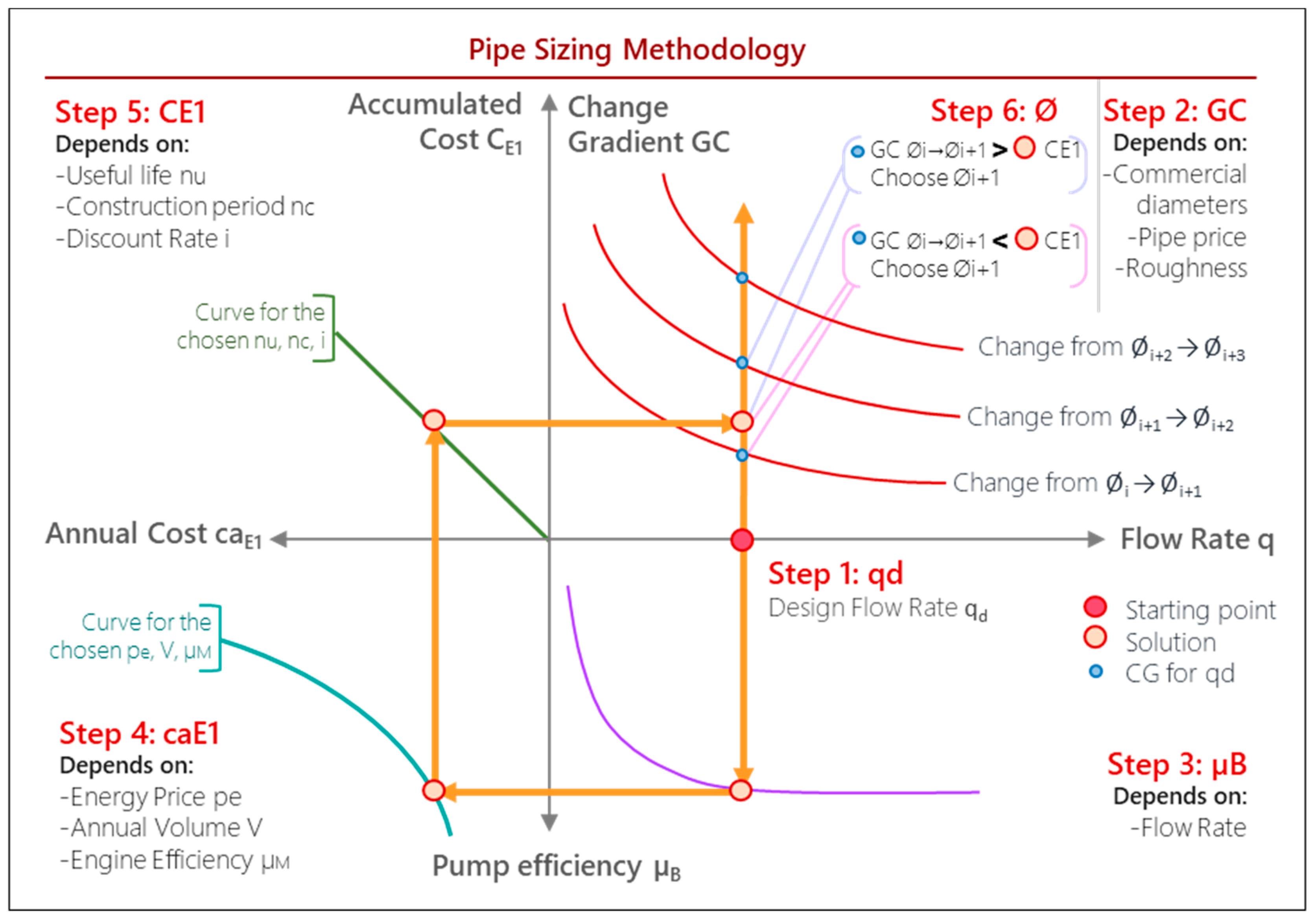
For a better comprehension, the full procedure is shown in Figure 7. On the figure, all variables affecting the change gradient and the energy cost are graphically represented: flow rate, pump efficiency, energy price, annual volume of water, engine efficiency, useful life of the installation, construction period, discount rate, commercial diameters, pipe prices and pipe roughness.
The design process represented in Figure 7 consists of the following steps:
- Calculate the design demand flow rate of the hydraulic drive.
- Calculate the change gradient curves for a commercial series of diameters with Equation (2).Since the aim is to compare the construction costs to those of the energy, excavation costs also must be considered and added to these figures.
- Calculate the expected pump efficiency using the average pump efficiency equation (Equation (7)).It is always more conservative to use the average pump efficiency equation rather than the maximum one, nevertheless this one can also be used but it would require a much more exhaustive pump search.
- Calculate the annual energy cost for one meter height Ca
- E1 using Equation (3).At this point, different alternatives might be considered for various energy prices, etc.
- Calculate the total accumulated energy cost for one meter height CE1 with Equations (3) and (4).
- Compare the change gradient and the energy cost CE1 and select the pipe diameter: when < CE1 select the wider diameter ; but when > CE1 select diameter . When = CE1, it is always preferable to build a bigger diameter , in case energy price, discount rate, etc. change.
3.3. Case Study: Navas del Marqués
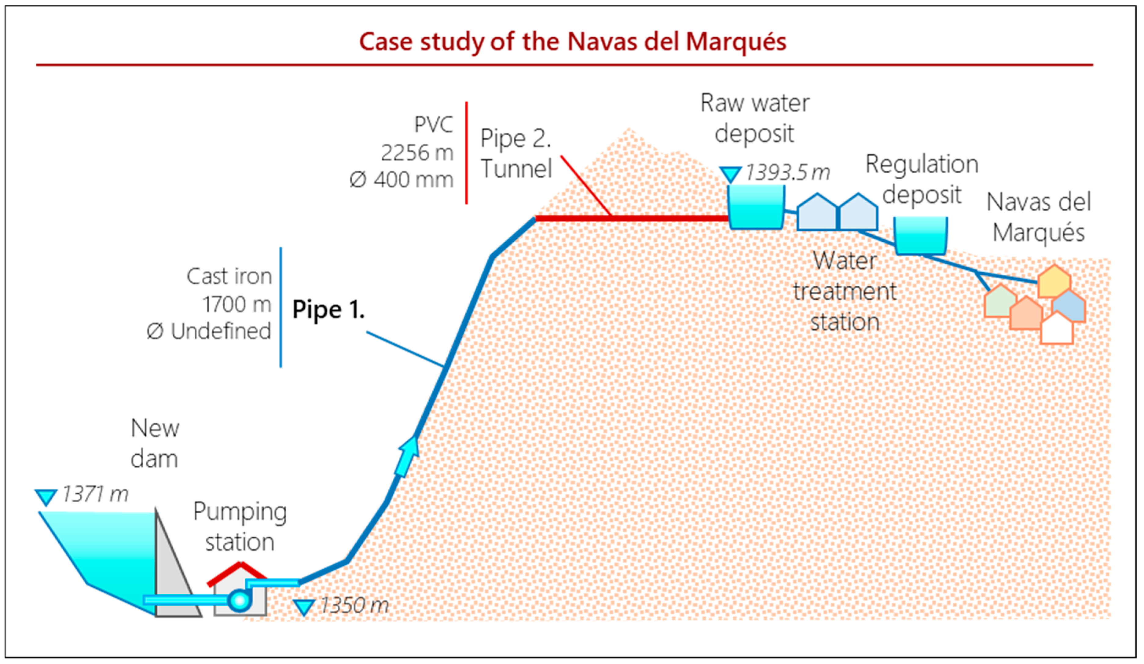
To exemplify the application of the previous design procedure, the method will be used in a case study. It is based on the dam project in the Navas del Marqués locality, Ávila, Spain, which was carried out by the Tagus Hydrographic Confederation [40]. In this section we intend to compare the design results obtained in the project to the ones that would be obtained with the proposed procedure. The project included the following works:
- New dam.
- New pumping station.
- New pipe replacing the first part of the water drive. There was a tunnel section from the previous water supply system that will remain as it was.
- New raw water deposit, previous to the water treatment station.
- New regulation deposit, after the water treatment station.
- New distribution network.
Figure 8 shows the schematic works that the project included, along with some relevant altitudes, and input data. This paper is concerned about the sizing of first part of the water drive, i.e., Pipe 1 (remember that the tunnel section, Pipe 2, was to remain in the original state).
The project data that are used can be summarized in the following list:
- Design flow rate: 0.164 m3/s.
- Annual volume of water: 1.5 hm3/year.
- Pipe diameters and the correspondent prices. These are compiled in Table 2.
- Energy price: 0.072 €/kWh.
- Duration of the construction period: 30 months.
- Although it is not specified in the project, pump engine efficiency is fixed at 94%.
This design process can be also followed throughout all series of Figure 9. These figures follow the same color code and symbology as Figure 7. The calculation followed the steps listed above:
- The design discharge flow is the one used by the original project which is q = 0.164 m3/s.
- For the calculation of the change gradients, the material for the pipe is ductile cast iron. Two different studies have been elaborated for two different pipe prices. Firstly, the pipe prices used in the project have been considered. Secondly, we used the pipe prices proposed by the Canal de Isabel II. Canal de Isabel II is the public authority in charge of the integral water supply of Madrid, Spain, and they published the average pipe prices they use in their infrastructure. Since the Tagus Hydrographic Confederation is also a public company, these prices have also been considered for a sensitivity analysis. On the other hand, it must be kept in mind that the prices used for the change gradient include that of the full construction cost (including excavation, joining, etc.). Table 2 shows the pipe prices and the change gradients.
- Using Equations (7) and (8), the average pump efficiency obtained is 82.44% and the maximum value is 86.52%. This same result can be obtained from Figure 6a with the design flow rate q = 0.164 m3/s.
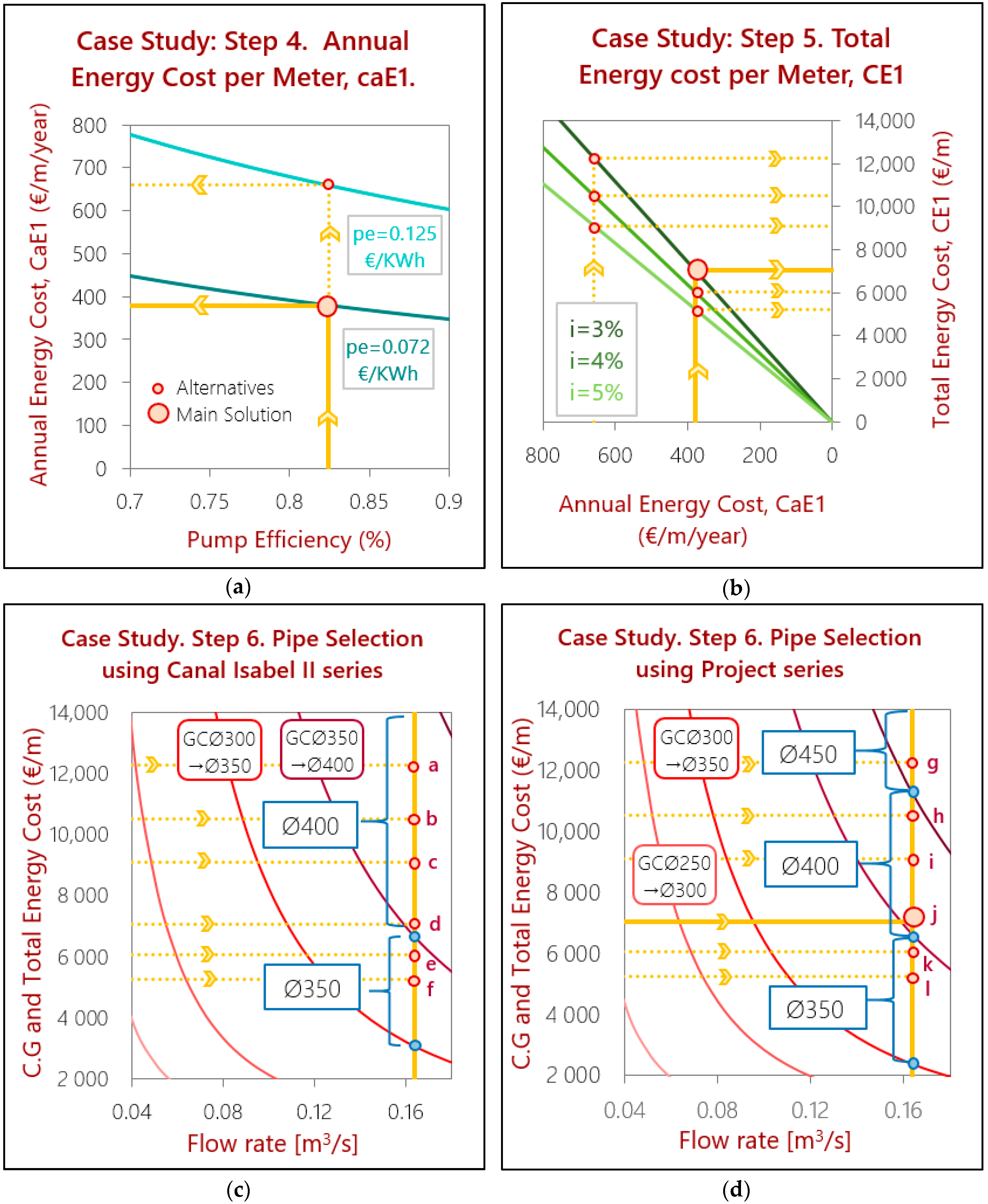
- The calculation of the annual energy cost per meter has been made for different values of the energy price. Engine efficiency was fixed at 94% and the demanded annual volume of the project is 1.5 hm3. Energy prices used for the calculations are 0.072 €/kWh, which, using Equation (3), gives an annual energy cost of 380 €/m/year; and also 0.125 €/kWh, for which CaE1 is 659 €/m/year.This will allow a sensibility analysis to see how robust the design is against energy price changes. The first price, 0.072 €/kWh, corresponds to the energy price used in the project, and the second alternative, 0.125 €/kWh, corresponds to a higher energy price. These results can be seen in Figure 9a.
- Once the annual unit pumping cost is obtained, the total accumulated cost is calculated using Equation (3). We assume a life span for the cast iron pipe of 31 years. Likewise, the duration of the expected construction period according to the project is 30 months, which corresponds to 2.5 years. We analyzed the sensibility of the design for the discount rate. In this line we adopt three values of the flow rate, where i equals 3%, 4% and 5%. With all this, the results obtained in each situation of energy prices and discount rate are shown in Table 3 below and in Figure 9b.
As it is shown, most of the alternatives throw back a pipe diameter solution of 400 mm; this is not too far from the solution taken in the project, which is 500 mm. The diameter selected in the project implies a facility with higher costs than the design obtained with the optimization of this research. However the project solution is energetically less consuming, and this is a positive fact because energy prices tend to increase with time, leading to significant increases in the energy cost. Nevertheless, when the sizing is made for project energy prices, the solutions oscillate between 350 and 400 mm. Although the project and presented method give close results, the new methodology can help to optimize the full cost of the facility.
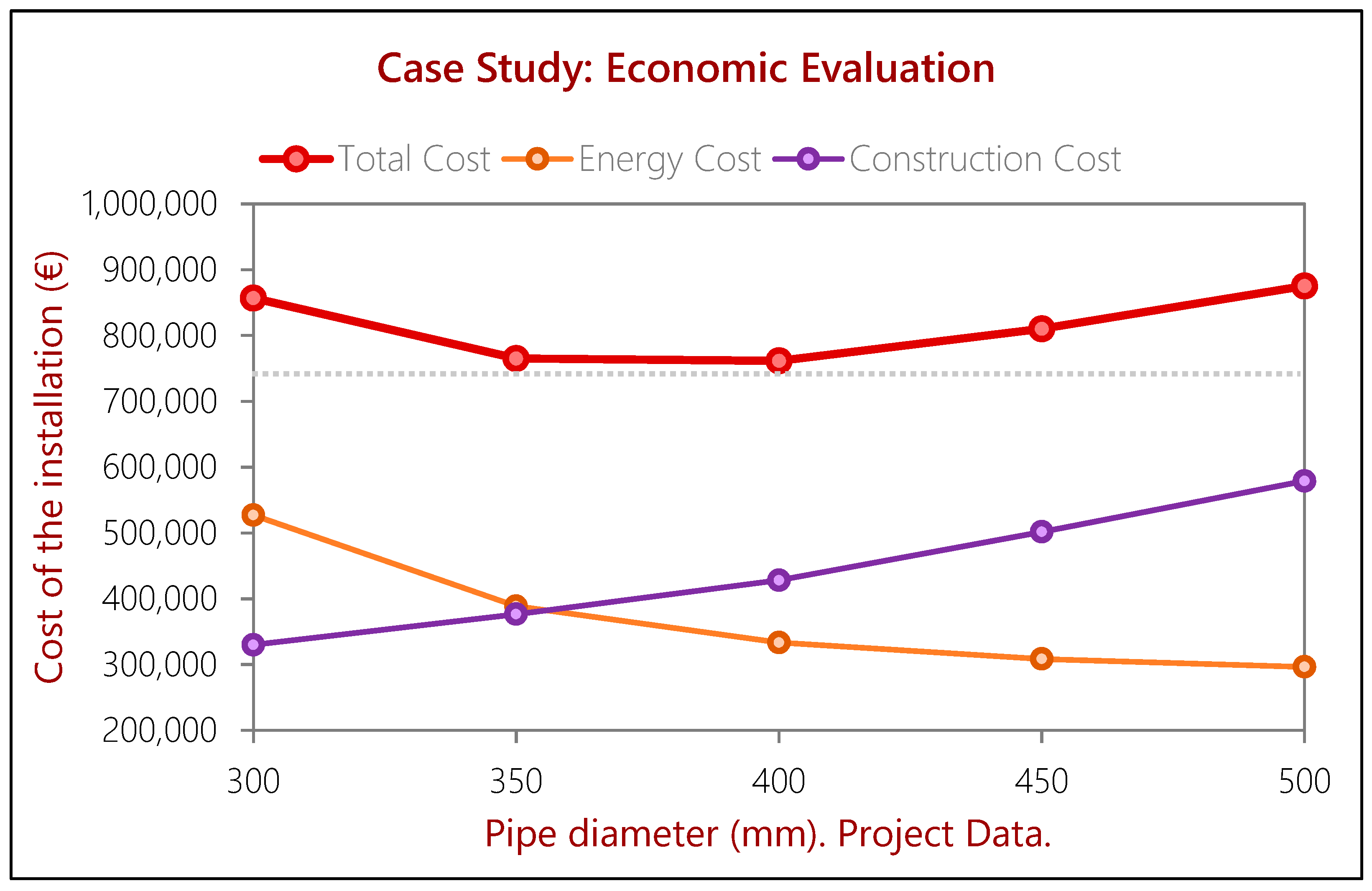
An economic evaluation has been conducted using the project energy prices and pipe prices. This can be seen in Table 4 and Figure 10.
Table 4 and Figure 10 show how diameters Ø400 mm and Ø350 mm give very close results for the total cost, since they only differ in approximately 4000 €. Nevertheless, the cost variation increases compared to diameter Ø500 mm and it is significantly higher, as it can be seen in Figure 10 even though the results only differ in 100 mm wide. When the sizing is made for higher energy prices, the most common result is 400 mm. As a conclusion, although the experience of the designer can never be replaced, this method is a very convenient tool to find the optimum diameter of a pipe.
4. Conclusions
The present pump analysis is a useful tool to help with the uncertainties regarding decision-making in water supply system design. Because the relationship of the pump efficiency with the other variables involved in the design process has been elucidated, the understanding of such a complex procedure as the design of a water supply system is improved.
The definition of the pump-efficiency–flow-rate curve reduces the conflict resolution involved in gradient-based methods, avoiding iterations regarding the pump efficiency. This automatically leads to less computational effort. In this sense, the Granados method is a straightforward procedure.
Some current methods are somewhat black-boxes, losing part of their utility by not being easy to comprehend for design engineers. The visual representation of our design methodology presented in this paper facilitates the understanding of the influence of each variable and allows to have a clear picture of the process. This simplicity is one of the main necessities to aim for when it comes to water supply system design.
As the case study shows, energy costs are proved to be a great fraction of the full cost of the installation, and they need to be considered from the first phase of the design. In contrast with other methodologies that do not consider these energy cost, this analysis aims for an integrated water assessment where all costs of the water–energy nexus are integrated.
Here, we obtain empirical equations that define the average and maximum optimal pump efficiency to expect depending on the flow rate of the installation. These results can be incorporated to elaborate a proper energy assessment of the operational costs. As the case study has shown, the design of a water supply system is also very much influenced by the construction costs (the design differs when Canal de Isabel II or project pipe prices are used) and by the energy rates (centesimal order variations will throw back different results). This reinforces the importance of carrying out a sensitivity analysis when it comes to designing a water supply system. These conclusions can be used for policy assessment in integrated water management as well as supply system design.
Author Contributions
Investigation, A.M.-C., D.S. and L.G. All authors have read and agreed to the published version of the manuscript.
Funding
This research was funded by CARLOS GONZÁLEZ CRUZ Grant.
Conflicts of Interest
The authors declare no conflict of interest.
References
- Sanchis, R.; Díaz-Madroñero, M.; López-Jiménez, P.A.; Pérez-Sánchez, M. Solution Approaches for the Management of the Water Resources in Irrigation Water Systems with Fuzzy Costs. Water 2019, 11, 2432. [Google Scholar] [CrossRef] [Green Version]
- Mala-Jetmarova, H.; Sultanova, N.; Savic, D. Lost in optimisation of water distribution systems? A literature review of system operation. Environ. Model. Softw. 2017, 93, 209–254. [Google Scholar] [CrossRef] [Green Version]
- Kim, J.H.; Mays, L.W. Optimal rehabilitation model for water-distribution systems. J. Water Resour. Plan. Manag. 1994, 120, 674–692. [Google Scholar] [CrossRef]
- Kang, D.; Lansey, K. Scenario-based robust optimization of regional water and wastewater infrastructure. J. Water Resour. Plan. Manag. 2012, 139, 325–338. [Google Scholar] [CrossRef]
- Dziedzic, R.; Karney, B.W. Cost gradient–based assessment and design improvement technique for water distribution networks with varying loads. J. Water Resour. Plan. Manag. 2015, 142, 04015043. [Google Scholar] [CrossRef]
- Samani, H.M.; Mottaghi, A. Optimization of water distribution networks using integer linear programming. J. Hydraul. Eng. 2006, 132, 501–509. [Google Scholar] [CrossRef]
- Costa, A.; De Medeiros, J.; Pessoa, F. Optimization of pipe networks including pumps by simulated annealing. Braz. J. Chem. Eng. 2000, 17, 887–896. [Google Scholar] [CrossRef]
- Vamvakeridou-Lyroudia, L.; Walters, G.; Savic, D. Fuzzy multiobjective optimization of water distribution networks. J. Water Resour. Plan. Manag. 2005, 131, 467–476. [Google Scholar] [CrossRef]
- Spiliotis, M.; Tsakiris, G. Minimum cost irrigation network design using interactive fuzzy integer programming. J. Irrig. Drain. Eng. 2007, 133, 242–248. [Google Scholar] [CrossRef]
- Jin, X.; Zhang, J.; Gao, J.-L.; Wu, W.-Y. Multi-objective optimization of water supply network rehabilitation with non-dominated sorting genetic algorithm-II. J. Zhejiang Univ. Sci. A 2008, 9, 391–400. [Google Scholar] [CrossRef]
- Roshani, E.; Filion, Y. Event-based approach to optimize the timing of water main rehabilitation with asset management strategies. J. Water Resour. Plan. Manag. 2013, 140, 04014004. [Google Scholar] [CrossRef] [Green Version]
- Perelman, L.; Ostfeld, A. An adaptive heuristic cross-entropy algorithm for optimal design of water distribution systems. Eng. Optim. 2007, 39, 413–428. [Google Scholar] [CrossRef]
- Perelman, L.; Ostfeld, A.; Salomons, E. Cross entropy multiobjective optimization for water distribution systems design. Water Resour. Res. 2008, 44. [Google Scholar] [CrossRef] [Green Version]
- Wu, W.; Simpson, A.R.; Maier, H.R. Multi-objective genetic algorithm optimisation of water distribution systems accounting for sustainability. Proc. Water Down Under 2008, 2008, 1750. [Google Scholar]
- Wu, W.; Simpson, A.R.; Maier, H.R. Accounting for greenhouse gas emissions in multiobjective genetic algorithm optimization of water distribution systems. J. Water Resour. Plan. Manag. 2009, 136, 146–155. [Google Scholar] [CrossRef] [Green Version]
- Wu, W.; Maier, H.R.; Simpson, A.R. Single-objective versus multiobjective optimization of water distribution systems accounting for greenhouse gas emissions by carbon pricing. J. Water Resour. Plan. Manag. 2009, 136, 555–565. [Google Scholar] [CrossRef] [Green Version]
- Wu, W.; Simpson, A.R.; Maier, H.R. Sensitivity of optimal tradeoffs between cost and greenhouse gas emissions for water distribution systems to electricity tariff and generation. J. Water Resour. Plan. Manag. 2011, 138, 182–186. [Google Scholar] [CrossRef] [Green Version]
- Wu, W.; Simpson, A.R.; Maier, H.R.; Marchi, A. Incorporation of variable-speed pumping in multiobjective genetic algorithm optimization of the design of water transmission systems. J. Water Resour. Plan. Manag. 2011, 138, 543–552. [Google Scholar] [CrossRef] [Green Version]
- Stokes, C.S.; Simpson, A.R.; Maier, H.R. A computational software tool for the minimization of costs and greenhouse gas emissions associated with water distribution systems. Environ. Model. Softw. 2015, 69, 452–467. [Google Scholar] [CrossRef]
- Stokes, C.S.; Maier, H.R.; Simpson, A.R. Effect of storage tank size on the minimization of water distribution system cost and greenhouse gas emissions while considering time-dependent emissions factors. J. Water Resour. Plan. Manag. 2015, 142, 04015052. [Google Scholar] [CrossRef] [Green Version]
- Reed, P.M.; Hadka, D.; Herman, J.D.; Kasprzyk, J.R.; Kollat, J.B. Evolutionary multiobjective optimization in water resources: The past, present, and future. Adv. Water Resour. 2013, 51, 438–456. [Google Scholar] [CrossRef] [Green Version]
- Carrasco, F.J.M.; de Marcos, L.G. Dimensionamiento y Optimización de Obras Hidráulicas, 4th ed.; Garceta Grupo Editorial: Malaga, Spain, 2013. (In Spanish) [Google Scholar]
- Granados, A. Problemas de Obras Hidráulicas; Escuela de Ingenieros de Caminos, Canales y Puertos. Servicio de Publicaciones: Madrid, Spain, 1995. (In Spanish) [Google Scholar]
- Ostfeld, A. Optimal design and operation of multiquality networks under unsteady conditions. J. Water Resour. Plan. Manag. 2005, 131, 116–124. [Google Scholar] [CrossRef]
- Gessler, J.; Walski, T.M. Water Distribution System Optimization; Army Engineer Waterways Experiment Station Vicksburg Ms Environmental Lab: Washington, DC, USA, 1985. [Google Scholar]
- Alperovits, E.; Shamir, U. Design of optimal water distribution systems. Water Resour. Res. 1977, 13, 885–900. [Google Scholar] [CrossRef]
- Featherstone, R.E.; El-Jumaily, K.K. Optimal diameter selection for pipe networks. J. Hydraul. Eng. 1983, 109, 221–234. [Google Scholar] [CrossRef]
- Dandy, G.; Hewitson, C. Optimizing hydraulics and water quality in water distribution networks using genetic algorithms. In Building Partnerships, Joint Conference on Water Resource Engineering and Water Resources Planning and Management 2000, Minneapolis, MN, USA, 30 July–2 August 2000; Hotchkiss, R.H., Glade, M., Eds.; ASCE: Reston, VA, USA, 2000; pp. 1–10. [Google Scholar]
- Tsakiris, G.; Spiliotis, M. Fuzzy linear programming for problems of water allocation under uncertainty. Eur. Water 2004, 7, 25–37. [Google Scholar]
- Gonçalves, G.M.; Gouveia, L.; Pato, M.V. An improved decomposition-based heuristic to design a water distribution network for an irrigation system. Ann. Oper. Res. 2014, 219, 141–167. [Google Scholar] [CrossRef]
- Marques, J.; Cunha, M.; Savić, D. Using real options in the optimal design of water distribution networks. J. Water Resour. Plan. Manag. 2014, 141, 04014052. [Google Scholar] [CrossRef] [Green Version]
- Schwartz, R.; Housh, M.; Ostfeld, A. Least-cost robust design optimization of water distribution systems under multiple loading. J. Water Resour. Plan. Manag. 2016, 142, 04016031. [Google Scholar] [CrossRef]
- Ostfeld, A.; Tubaltzev, A. Ant colony optimization for least-cost design and operation of pumping water distribution systems. J. Water Resour. Plan. Manag. 2008, 134, 107–118. [Google Scholar] [CrossRef]
- Vicente, D.; Garrote, L.; Sánchez, R.; Santillán, D. Pressure management in water distribution systems: Current status, proposals, and future trends. J. Water Resour. Plan. Manag. 2015, 142, 04015061. [Google Scholar] [CrossRef]
- Capelo, B.; Pérez-Sánchez, M.; Fernandes, J.F.; Ramos, H.M.; López-Jiménez, P.A.; Branco, P.C. Electrical behaviour of the pump working as turbine in off grid operation. Appl. Energy 2017, 208, 302–311. [Google Scholar] [CrossRef]
- Tsakiris, G.; Spiliotis, M. Uncertainty in the analysis of urban water supply and distribution systems. J. Hydroinform. 2017, 19, 823–837. [Google Scholar] [CrossRef] [Green Version]
- Fu, G.; Kapelan, Z.; Reed, P. Reducing the complexity of multiobjective water distribution system optimization through global sensitivity analysis. J. Water Resour. Plan. Manag. 2011, 138, 196–207. [Google Scholar] [CrossRef]
- Pérez-Sánchez, M.; Sánchez-Romero, F.-J.; López-Jiménez, P.A. Huella energética del agua en función de los patrones de consumo en redes de distribución. Ingeniería Agua 2017, 21, 197–212. [Google Scholar] [CrossRef] [Green Version]
- Pérez-Sánchez, M.; López-Jiménez, P.A.; Ramos, H.M. Modified affinity laws in hydraulic machines towards the best efficiency line. Water Resour. Manag. 2018, 32, 829–844. [Google Scholar] [CrossRef] [Green Version]
- Cabreros, J.M. Proyecto de Presa Navas del Marqués; Tajo, C.H.d., Ed.; Ministerio de Medio Ambiente: Ávila, Spain, 1999. (In Spanish)
Figure 1.
(a). Optimum pump efficiency and the correspondent flow rate at that operating point, classified by the pump type. (b) Detail of the previous figure for smaller discharges.
Figure 1.
(a). Optimum pump efficiency and the correspondent flow rate at that operating point, classified by the pump type. (b) Detail of the previous figure for smaller discharges.

Figure 2.
Optimum pump efficiency and the correspondent pumping height at that operating point.

Figure 3.
(a) Optimum pump efficiency and the correspondent pump power at that operating point. (b) Detail of the previous figure.
Figure 3.
(a) Optimum pump efficiency and the correspondent pump power at that operating point. (b) Detail of the previous figure.

Figure 4.
Optimum pump efficiency and the correspondent specific speed of the pump, classified by the pump type.
Figure 4.
Optimum pump efficiency and the correspondent specific speed of the pump, classified by the pump type.

Figure 5.
Adjusted curves. The curves are elaborated using 14 intervals of the collected data.

Figure 6.
(a) Optimum pump efficiency curve: database and mathematical adjustment; (b) mathematical adjustment in logarithmic scale.
Figure 6.
(a) Optimum pump efficiency curve: database and mathematical adjustment; (b) mathematical adjustment in logarithmic scale.

Figure 7.
Pipe sizing methodology representing the steps for the design and the shapes that curves might present depending on the variables.
Figure 7.
Pipe sizing methodology representing the steps for the design and the shapes that curves might present depending on the variables.

Figure 8.
Case study at Navas del Marqués.: Pipe 1 is the only one to replace.

Figure 9.
Case study of the Navas del Marqués. (a) Step 4: Calculation of the annual energy cost; (b) Step 5: Calculation of the capitalized energy cost throughout the entire life of the installation. (c,d) Both panels show steps 1 and 5 of the procedure. This means that both the change gradient calculation (red curves) and the pipe selection is shown in the figures. In (c), the change gradients are calculated using the Canal de Isabel II commercial diameters, and in (d), they used the project data. The big orange circle in (d) represents the main solution, whilst the small orange circles represent the solutions for the other alternatives evaluated in the case study. For the main solution, as the energy cost per meter CE1 is greater than CGØ350→Ø400, it is more convenient to choose Ø400 mm. But because CE1 is smaller than CGØ400→Ø450, it should not be passed onto Ø450 mm and remain with Ø400 mm. The same reasoning applies to the other solution alternatives.

Figure 10.
Economic evaluation of the case study at the Navas del Marqués.


Table 1.
Elaboration of the adjusted curves of the pump efficiency versus the flow rate.
| Pump Efficiency for Each Flow Rate Interval | ||||||
|---|---|---|---|---|---|---|
| Interval Number | Flow Rate Range | Pump Efficiency | ||||
| Minimum | Maximum | Average | Average | Maximum | Minimum | |
| q (L/s) | q (L/s) | q (L/s) | µB (%) | µB (%) | µB (%) | |
| 1 | 0 | 5 | 2.5 | 55.3% | 77.0% | 36.2% |
| 2 | 5 | 10 | 7.5 | 63.5% | 76.0% | 45.0% |
| 3 | 10 | 15 | 12.5 | 65.7% | 77.0% | 45.0% |
| 4 | 15 | 25 | 20 | 74.2% | 82.0% | 63.0% |
| 5 | 25 | 40 | 32.5 | 75.0% | 85.0% | 61.2% |
| 6 | 40 | 65 | 52.5 | 78.6% | 84.0% | 70.5% |
| 7 | 65 | 100 | 82.5 | 81.0% | 85.4% | 75.4% |
| 8 | 100 | 150 | 125 | 83.1% | 86.0% | 74.0% |
| 9 | 150 | 200 | 175 | 82.8% | 87.0% | 80.4% |
| 10 | 200 | 300 | 250 | 83.9% | 88.0% | 81.0% |
| 11 | 300 | 500 | 400 | 84.9% | 88.8% | 79.9% |
| 12 | 500 | 1000 | 750 | 85.5% | 88.5% | 80.4% |
| 13 | 1000 | 2000 | 1500 | 88.3% | 89.0% | 86.7% |
| 14 | 2000 | 3000 | 2500 | 88.2% | 89.0% | 86.2% |
Table 2.
Pipe prices series and change gradients calculations.
| Change Gradients | ||||
|---|---|---|---|---|
| Pipe Diameter | Canal de Isabel II | Project Diameters | ||
| Construction Cost | Change Gradient | Construction Cost | Change Gradient | |
| mm | €/m | €/m | €/m | €/m |
| 60 | 55 | 0.11 | ||
| 80 | 64 | 0.26 | ||
| 100 | 69 | 2.11 | ||
| 125 | 79 | 4.84 | ||
| 150 | 86 | 30 | 103 1 | 36 |
| 200 | 105 | 233 | 127 | 256 |
| 250 | 134 | 796 | 159 | 1044 |
| 300 | 161 | 3070 | 194 | 2373 |
| 350 | 197 | 6670 | 221 | 6593 |
| 400 | 227 | 15,972 | 252 | 11,226 |
| 450 | 260 | 33,781 | 295 | 64,309 |
| 500 | 295 | 98,565 | 341 | 76,920 |
| 600 | 378 | 405 | ||
1 The project includes a limited series of ductile cast iron pipes in the estimated budget documents. These start from 150 mm.
Table 3.
Selection of the pipe diameter, depending on the energy prices, diameter series and discount rate considered.
Table 3.
Selection of the pipe diameter, depending on the energy prices, diameter series and discount rate considered.
| Pipe Selection | ||||||
|---|---|---|---|---|---|---|
| Annual Unit Energy Cost | Total Unit Energy Cost | Selected Diameter | ||||
| Energy Price | CaE1 | i | fa | CE1 | Canal Isabel II Pipes | Project Pipes |
| €/m/year | % | €/m | mm | mm | ||
| 0.125 €/kWh | 659 | 3 | 18.6 | 12,248 | (a) 400 * | (g) 450 |
| 4 | 15.9 | 10,513 | (b) 400 | (h) 400 | ||
| 5 | 13.8 | 9100 | (c) 400 | (i) 400 | ||
| 0.072 €/kWh | 380 | 3 | 18.6 | 7055 | (d) 400 | (j) 400 |
| 4 | 15.9 | 6056 | (e) 350 | (k) 350 | ||
| 5 | 13.8 | 5242 | (f) 350 | (l) 350 | ||
* The letters in brackets indicate the graphical solutions in Figure 9c,d.
Table 4.
Economic evaluation for the case study using the project prices for the pipes, once a diameter of 400 mm has been selected, to prove the least cost result.
Table 4.
Economic evaluation for the case study using the project prices for the pipes, once a diameter of 400 mm has been selected, to prove the least cost result.
| Economic Evaluation | |||||
|---|---|---|---|---|---|
| Diameter | Construction Costs | Head Loss | Annual Cost | i = 3% | Total Cost |
| Ø | ∆h | caE | CE | ||
| (mm) | € | (m) | (€/year) | (€) | (€) |
| 300 | 329,886 | 35.01 | 28,374 | 527,076 | 856,962 |
| 350 | 376,444 | 15.39 | 20,922 | 388,646 | 765,091 |
| 400 | 428,121 | 7.55 | 17,946 | 333,353 | 761,474 |
| 450 | 501,646 | 4.03 | 16,609 | 308,516 | 810,162 |
| 500 | 578,985 | 2.30 | 15,951 | 296,302 | 875,288 |
© 2019 by the authors. Licensee MDPI, Basel, Switzerland. This article is an open access article distributed under the terms and conditions of the Creative Commons Attribution (CC BY) license (http://creativecommons.org/licenses/by/4.0/).
Share and Cite
MDPI and ACS Style
Martin-Candilejo, A.; Santillán, D.; Garrote, L. Pump Efficiency Analysis for Proper Energy Assessment in Optimization of Water Supply Systems. Water 2020, 12, 132. https://doi.org/10.3390/w12010132
AMA Style
Martin-Candilejo A, Santillán D, Garrote L. Pump Efficiency Analysis for Proper Energy Assessment in Optimization of Water Supply Systems. Water. 2020; 12(1):132. https://doi.org/10.3390/w12010132
Chicago/Turabian StyleMartin-Candilejo, Araceli, David Santillán, and Luis Garrote. 2020. "Pump Efficiency Analysis for Proper Energy Assessment in Optimization of Water Supply Systems" Water 12, no. 1: 132. https://doi.org/10.3390/w12010132
Note that from the first issue of 2016, this journal uses article numbers instead of page numbers. See further details here.