Vertical Distribution of Suspended Sediments above Dense Plants in Water Flow

Abstract

Plants in natural water flow can improve water quality by adhering and absorbing the fine suspended sediments. Dense plants usually form an additional permeable bottom boundary for the water flow over it. In the flow layer above dense plants, the flow velocity generally presents a zero-plane-displacement and roughness-height double modified semi-logarithmic profile. In addition, the second order shear turbulent moment (or the Reynolds stress) are different from that found in non-vegetated flow. As a result, the turbulent momentum diffusivity of flow and thus the diffusivity of sediment will shift, which will cause the vertical profile of suspended sediment and the corresponding Rouse formula deform. A set of physical experiments with three different diameters of fine suspended sediments was conducted in an indoor water flume. These experiments investigated a new distribution pattern of suspended sediment and the correspondingly deformed Rouse formula in the flow layer over the dense plants. Experimental results showed that above the dense plants, the shear turbulent momentum of flow presented a plant-height modified negative linear profile, which has been proposed by a previous study, and the vertical distribution of fine suspended sediments presented an equilibrium pattern. Based on the plant-modified profiles of flow velocity and the shear turbulent momentum a new zero-plane and plant-height double modified Rouse formula were analytically derived. This double-parameter modified Rouse formula agrees well with the measured profile of suspended sediment concentration experimentally observed in the present study. By adjusting the Prandtl–Schmidt number, i.e., the ratio of sediment diffusivity to flow diffusivity, the double-parameter modified Rouse formula can be applied to submerged dense plant occupied flow.

1. Introduction

Aquatic plants in natural water flow as are present in a river, lake or reservoir is usually used as a key phytoremediation element in eco-restoration projects because of its many benefits to an aquatic environment [1,2,3]. The beneficial effects of aquatic plants on the deposition, retention and filtration of suspended sediment in the deep part of a flow due to the plants’ extensive root system has been widely acknowledged [4,5,6,7]. In the above-plant region, aquatic plants also influence the transport and movement of fine suspended sediment. These fine suspended sediments increase water turbidity, prevent photosynthesis in plants, affect the accessibility of food for larvae, and impact the quality of the aquatic habitat [8,9]. Consequently, understanding of the vertical distribution pattern of suspended sediments in the above-plant region is important for developing our understanding the aquatic eco-system.

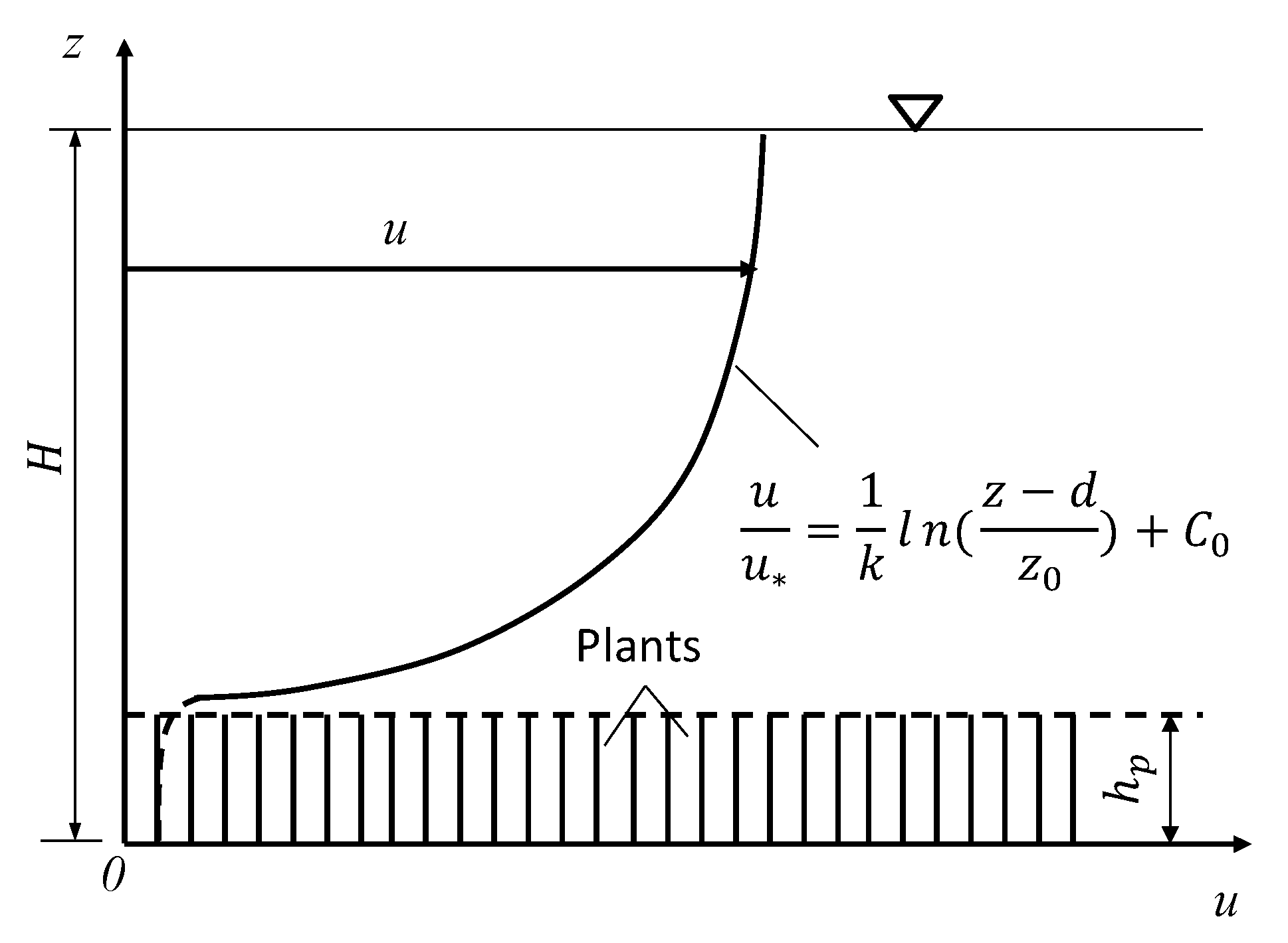
In a natural water flow environment, aquatic plants usually grow in dense groups on the flow bed, thereby forming an additional permeable bottom boundary for the flow layer above it. The flow shear, i.e., the vertical gradient of flow velocity ($du/dz$) presents a remarkable two-layer feature in the within-plant region and the over-plant region [10,11,12,13]. In the within-plant region, the flow shear ($du/dz$) is approximately zero, as the velocity profile is constant. In the over-plant region, the flow shear ($du/dz$) no longer follows the traditional logarithmic law of the non-planted bare-bed flow, but is usually modeled by a deformed logarithmic law [14]. For dense submerged plant occupied flow, some studies have acknowledged that the traditional logarithmic law can be modified with the assistance of two parameters: the zero-plane-displacement ($d$) and the roughness height ($z_0$; Figure 1). Researchers have proposed various expressions for $d$ and $z_0$ [15,16,17,18]. Stephan and Gutknecht (2002) [14] have given a detailed summary of these expressions. The $d$ and $z_0$ modified flow shear ($du/dz$; $u$ is the time-averaged flow velocity in streamwise direction) causes direct changes in the profile of the momentum diffusivity of flow (${\epsilon }_m=-\overline{u^{\prime }{w}^{\prime }}/\left(du/dz\right)=\tau /\left(\rho ·du/dz\right)$, $u^{\prime }$ and $w^{\prime }$ are perturbations of flow velocity in streamwise and vertical directions), which will cause changes in the distribution pattern of suspended sediments (e.g., [19]).

Another important parameter that influences the turbulent diffusivity of flow (${\epsilon }_m$) and sediment (${\epsilon }_s$), and thus influences the distribution patter of suspended sediment is the second order shear turbulent momentum ($-\overline{u^{\prime }{w}^{\prime }}$, which is usually used to represent the Reynolds stress, $\tau =-\rho \overline{u^{\prime }{w}^{\prime }}$). It is widely acknowledged that ($-\overline{u^{\prime }{w}^{\prime }}$) reaches a maximum value around the top of the plants, and then decreases upward towards the surface of the water [20,21,22]. Based on this feature, Li et al. (2018) [23] assumed that in the flow layer above the submerged plant, the shear stress follows the Vanoni profile ($\tau =\rho gS\left(H-z\right)$, $S$ is the energy slope; $H$ is the water depth), and that the flow velocity follows a $d$–$z_0$ double modified logarithmic-law profile. Based on these assumptions, they then derived the parabolic profile of ${\epsilon }_m$, which resulted in a profile of the $ln$-form of the suspended sediment concentration ($ln\left(C_s\right)$, $C_s$ is the concentration of suspended sediment). However, a further direct formula for suspended sediment concentration ($C_s$) has not been derived due to the complexity of the expression of $ln\left(C_s\right)$.

Based on the generally upward-decreasing feature of the profile of ${\epsilon }_m$, Huai et al. (2019) [24] assumed a zero-value of ${\epsilon }_m$ at the water surface, and then assumed a linear profile of ${\epsilon }_m$ between the water surface and the plant top. They successfully created a random displacement model for the prediction of the profile of the suspended sediment concentration profile $(C_s)$. Yang and Choi (2010) [25] assumed ${\epsilon }_m$ to be parabolic, and derived a parabolic Rouse formula for suspended sediment concentration, which is modified by the plant height.

The previous models and formulae for the prediction of suspended sediment concentration ($C_s$) are all based on the equilibrium mechanism of the dynamic balance between upward turbulent diffusion and downward gravitational settling, i.e., the convection–diffusion equation. Based on this equilibrium mechanism, Rouse (1937) [26] derived the Rouse formula with the turbulent diffusion being expressed by Fick’s first law. Fredsøe and Deigaard (1992) [27] derived the Vanoni formula with the turbulent diffusion being expressed by a mixing length involved term. These two formulae have the same expression. For flow through submergent plants, several different deformed Rouse formulae have been derived under some particular flow, sediment and plant conditions. However, investigation of the profile of suspended sediment in the flow layer above aquatic plants is still limited. Correspondingly, models to predict sediment and plant in this flow layer are also limited.

Fine sediment is commonly observed to be deposited on the foliage of submerged dense plants after a flood or storm. However, the mechanism by which he foliage-deposited sediment diffuses or is transported in the steady high-level flow after a flood has rarely been reported. The objectives of the present study are: (1) to investigate the profile of suspended sediment concentration ($C_s$) in dense plant occupied flow under a high submergence ratio, with suspended sediment coming from upstream instead of coming upwards from the flow bed; (2) to seek suitable formulae of the profiles of flow shear ($du/dz$) and the shear turbulent momentum ($-\overline{u^{\prime }{w}^{\prime }}$); and (3) to derive an analytical formula of the profile of suspended sediment concentration (i.e., a deformed Rouse formula). The results are expected to compensate for the limited data of $C_s$-profile over dense plants, and to provide fundamental guidance for the design of phytoremediation of eco-restoration projects in natural water flow.

2. Experimental Setup and Methods

2.1. Water Flume and Co-Ordinate System

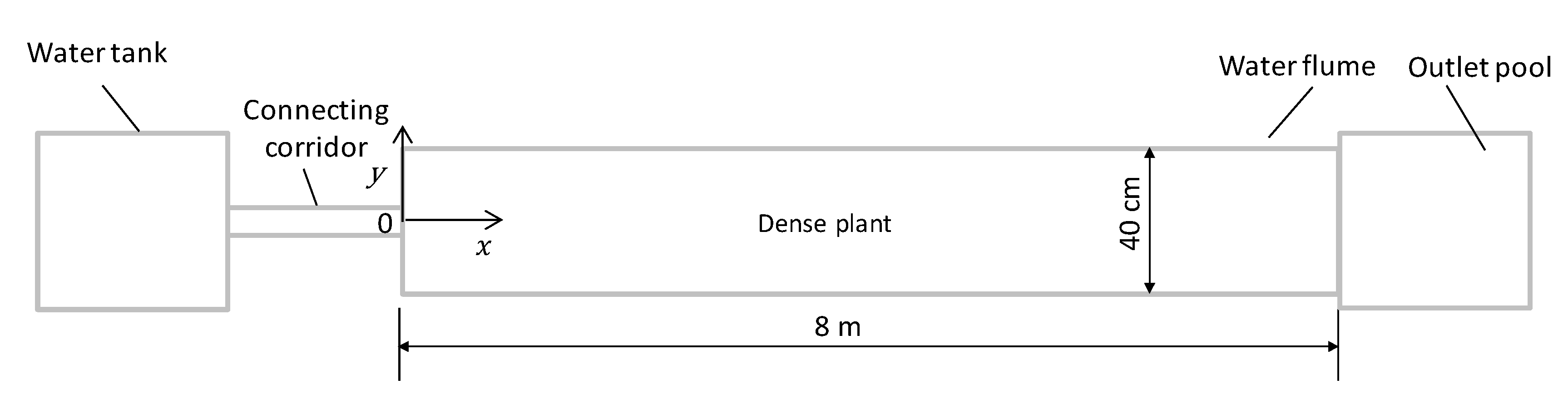
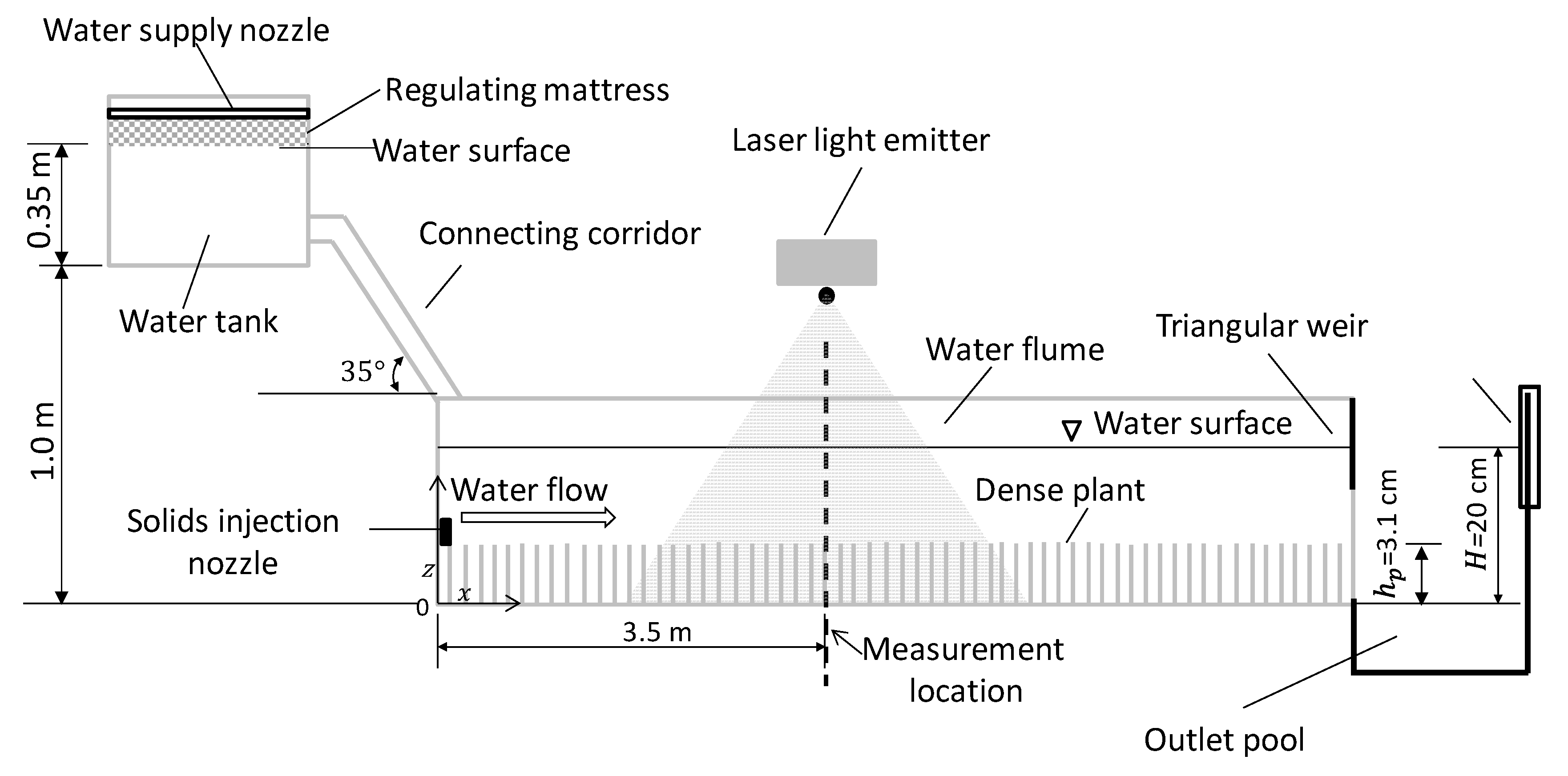
A rectangular water flume was used to conduct a set of indoor physical experiments. The flume was 8 m long, 40 cm wide, and 40 cm high (Figure 2 and Figure 3). To conveniently observe the configuration of plants, the water surface, and the concentration of fine suspended sediments, large pieces of transparent glass were embedded in aluminum frames for two side-walls of the water flume. A 1 m × 1 m × 0.5 m water tank was set up at the upstream end of the flume. The water was supplied from a flat nozzle, and the polymer-sponge mattress was placed on the water surface to minimize the fluctuation of the water surface in the tank (Figure 3). The water tank was installed on a bracket, so that the bottom of the water tank was 1.0 m above the bottom of the flume (Figure 3). The water tank was connected to the water flume with an upper-surface-open corridor. The connecting corridor was 38 cm wide, 40 cm high, and had a 35° tilt with respect to the horizontal. A valve was set at the upstream end of the corridor to adjust flow discharge in the corridor. Flow in the flume was driven by the water head between the water surface in tank and that in the flume. For all the experiments, water depth in the tank was maintained at 0.35 m. The water in the tank was supplied from a pipe. To adjust flow depth ($H$) and measure flow discharge ($Q$), a triangular wire was set at the downstream end of the flume (Figure 3). An outlet pool with an outlet valve was connected to the flume at the downstream edge of the flume (Figure 2 and Figure 3).

The co-ordinate system is shown in Figure 2 and Figure 3. The origin point in the co-ordinate system was located at the intersection of the upstream edge and the streamwise center line of the flume bottom.

2.2. Plant Configurations

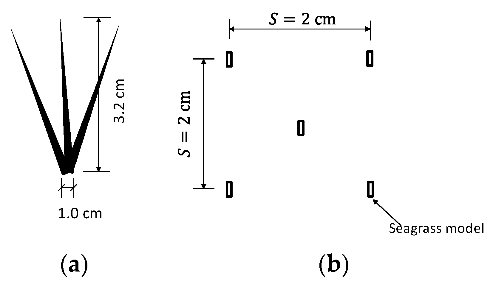
The plants were made of plastic. This allowed an imitation of a natural plant, since the material was flexible enough to allow the artificial plants to sway slightly in flow. The plant was designed as triple foliage, with each foliage having a thin plate shape. The plant foliage was 3.2 cm high and 1.2 mm thick (Figure 4a). In the present study, the time-space double averaged height of swaying plant $h_p=3.1$ cm. Therefore, the submergence ratio of plant $H/h_p>5$, which allowed the dense plants to form a permeable bottom boundary for flow.

The plants were installed on the flume bed in a staggered distribution pattern (Figure 4b), with the space between two neighbor plants $S=2 \mathrm{cm}$. The plants occupied the entire flume bed from $x=0$ m to the downstream end of flume. The frontal projected area of submerged vegetation per bed area ${\lambda }_f$ [28] is an important factor used to classify the density of canopy. Nepf (2012) [11] proposed a reference value, ${\lambda }_f=0.1$, to identify the dense canopy needed to generate inflected velocity profile based on experimentally measured data. In the present study ${\lambda }_f=0.775$, which is in the range of dense plants. In the present study, a high submergence ratio, combined with the dense distribution of plants on the bottom of the flow, ensured that the plants formed a permeable boundary. Therefore, flow velocity could be modeled as a modified logarithmic law.

2.3. Bulk Flow Condition and Fine Suspended Sediment Model

Bed slope ($S_b$) of the flume was adjusted at 0.38‰ to keep the experimental flow in a quasi-steady condition. During the total four sets of experiments in the present study, the flow discharge ($Q$) was kept at a constant value of 0.0096 m³/s, and the flow depth ($H$) was 20 cm (

Table 1. Parameters of bulk flow and plant.

$\mathit{Q}$ (m3 s−1)	$\mathit{H}$ (cm)	$\mathit{V}$ (m s−1)	${\mathit{S}}_{\mathit{b}}$	${\mathit{u}}_{*}$ (cm s−1)	${\mathit{h}}_{\mathit{p}}$ (cm)	$\mathit{H}/{\mathit{h}}_{\mathit{p}}$	${\mathit{\lambda }}_{\mathit{f}}$
0.0096	20	0.12	0.00038	1.89	3.1	6.45	0.775

).

The fine suspended sediment was modeled as spherical balls made of plexiglass. Three different diameters of fine sediments were used: $d_s=36$, 59, and 80 $\mathsf{\mu }\mathrm{m}$. Three different specific gravities were used for these different diameters of sediment (

Table 2. Parameters of fine suspended sediments.

Cases	${\mathit{d}}_{\mathit{s}}$$\left(\mathsf{\mu }\mathbf{m}\right)$	${\mathit{r}}_{\mathit{s}}$	${\mathit{\omega }}_{\mathit{s}}$ (mm s−1)	${\mathit{u}}_{*}/{\mathit{\omega }}_{\mathit{s}}$	${\mathit{C}}_{\mathit{a}}$ (g L−1)
$d_{s1}$	36	1.866	0.84	22.5	0.18
$d_{s2}$	59	2.100	2.26	8.4	0.23
$d_{s3}$	80	2.164	4.16	4.5	0.28

Note: the variable $C_a$ represents the concentration of suspended sediment measured at the height level of 1.1 $h_p$, which is used as the reference concentration in the present study.

). The concentration profile of the fine suspended sediments was measured at $x=3.5$ m (Figure 3). The fine sediment was injected into the experimental flow from the upstream edge of the flume. The center of the injection nozzle was aligned with the center of cross direction of the flume, at a height equal to that of the top of the plants, i.e., at $z=3.2$ cm.

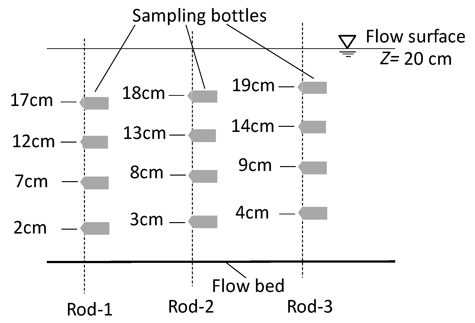
Sampling of suspended sediments was taken by a 95 mL sampling bottle over 35 s. Three sampling runs were conducted, with the first run starting from 5 min, the second run from 30 min and the third run from 45 min after the flow surface line became steady. In each sampling run three rigid rods were separately applied in order. Each rod had four sampling bottles attached. The spacing between the bottles was 5 cm for Rod_1 and Rod_3, and 6 cm for Rod_2 (Figure 5). Thus 12 measurement points along a vertical line were obtained. The volume concentration (g/L) of sediment was obtained by the filtering method. This sampling bottle was calibrated with the standard sampling bottle.

2.4. Measurement of Flow Velocity and the Observation of Plant Swaying

To obtain time-averaged mean and turbulent flow characteristics of flow, three-dimensional time series of flow velocity was observed by Acoustic Doppler Velocimeter (ADV). Time series of 3-D flow velocities along a vertical profile were measured in the middle section at $x=3.5$ m. The time-averaged flow velocities $u$ and $w$ ($u=U-u^{\prime }$, $w=W-w$, $U$ and $W$ are the instantaneous flow velocities in streamwise and vertical directions, respectively; $u^{\prime }$ and $w^{\prime }$ are the corresponding velocity perturbations) and the second order turbulent momentum ($-\overline{u^{\prime }{w}^{\prime }}$) were calculated from the measured time series of velocity. The recording frequency of the ADV was $f_R=25 \mathrm{Hz}$.

The recorded signal was filtered and de-spiked by the acceleration method and the phase-space threshold method [29]. We fed particles into the flow; thus, the spikes in the measured time series were not significant. For all the experimental tests, the filtered and de-spiked valid digital records of each time series were greater than 85%. The correlation coefficient falling in the range of [80, 95], and the ratio of signal to noise (SNR) was in the range of [15.0, 26.3] dB.

A laser emitter was hung over the flume to generate a thin sheet of laser light with a thickness of 1.5 mm in the $x-z$ plane along the longitudinal centerline of the flume (Figure 3). A video camera was fixed outside the glass window of the flume with the lens normal to the center of the laser light sheet (Figure 3). During each testing period, the dynamic movement of the plants was recorded by the camera. Thus, the time-averaged height of the plants was obtained by analyzing the sequential video via the computer.

2.5. Diffusivities of Momentum of Flow and Fine Suspended Sediments

The momentum diffusivity (i.e., diffusion coefficient) of flow is defined as

$${\epsilon }_m\equiv \left(-\overline{u^{\prime }{w}^{\prime }}\right)/\left(du/dz\right).$$

(1)

The diffusivity of fine suspended sediments is defined as

$${\epsilon }_s\equiv \beta {\epsilon }_m,$$

(2)

where $\beta$ is the Prandtl–Schmidt number. A $\beta$-value of unity is widely used. In applications, the Prandtl–Schmidt number is dependent on flow conditions as well as sediment and plant conditions.

2.6. Settling Velocity of Fine Suspended Sediments

The settling velocity of fine sediments (${\omega }_s$) is an important parameter for the determination of its distribution pattern. Since the dynamics of fine suspended sediments is influenced by turbulent dissipation, the modified formula of ${\omega }_s$ under turbulent flow condition was applied [30]:

$${\omega }_s={\omega }_{stokes}+\gamma k{u}_{*},$$

(3)

where ${\omega }_{stokes}=\left(1/18\right)\left[\left(r_s-r\right)/r\right]\left(g{d}^2/\nu \right)$ is the Stokes settling velocity of fine sediment in still water; $r$ is the specific gravity of water, $r=1$; $v$ is the kinematic viscosity of water, $v=1.004 \times {10}^{-6}{ \mathrm{m}}^2{\mathrm{s}}^{-1}$ at 20 °C; $\gamma$ is a modification coefficient, $\gamma =0.034$; and $k$ is the Karman constant, the standard value $k=0.4$ is used in the present study. The settling velocities of three fine sediments are given in Table 2. For the three diameters of sediment used in the present study the ratios of $u_{*}/{\omega }_s$ are greater than unity (Table 2), suggesting the fine sediments can be suspended [31,32].

Since the dense plants act as a new permeable boundary for the above flow, the shear velocity ($u_{*}$) was calculated from the value of $-\overline{u^{\prime }{w}^{\prime }}$ at the top of the plants, which is expressed by:

$$u_{*}=\sqrt{{(-\overline{u^{\prime }{w}^{\prime }})}_{plant\_top}}.$$

(4)

3. Results

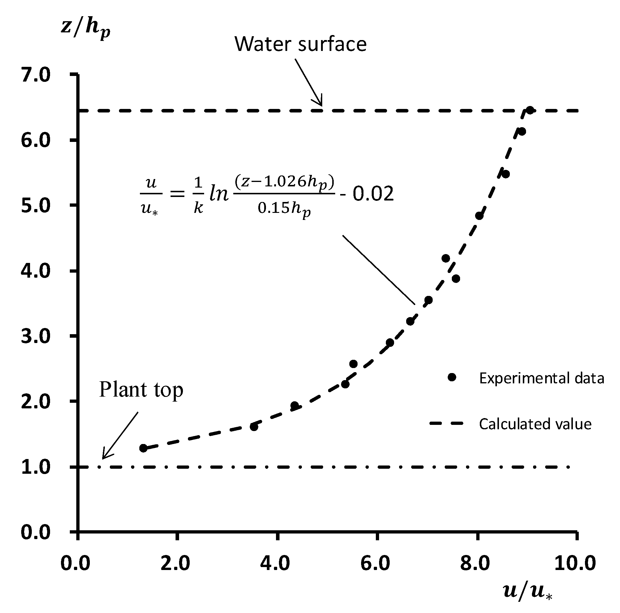
3.1. Vertical Velocity Profile

Figure 6 shows that with the dense plants acting as permeable bottom boundary, the over flow velocity follows a semi-logarithmic law modified by $d$ and $z_0$:

$$u/u_{*}=\frac{1}{k}\ln \left(\frac{z-d}{z_0}\right)+C_0,$$

(5)

where $k$ is the von Karman constant (the standard value $k=0.4$ was used in the present study); $\rho$ is the density of water; $d$ is the zero-plane displacement; $z_0$ is the roughness height; and $C_0$ is a constant.

In applications, the values of $d$, $z_0,$ and $C_0$ depend on the specified flow environment and plant configuration. For example, Stephan and Gutknecht (2002) [14] reported that both $d$ and $z_0$ take the average value of swaying plant height, that is, $d/h_p=1.0$, $z_0/h_p=1.0$, and $C_0=8.5$; Nezu and Sanjou (2008) [22] reported that the value of $z_0/h_p$ falls within the range of $\left[0.15, 0.17\right]$ and $C_0=0$ in their experiments.

In the present study, $d/h_p=1.026$, $z_0/h_p=0.15$, and $C_0=-0.02$. Therefore, the formula for the present study is:

$$u/u_{*}=\frac{1}{k}\ln \frac{\left(z-1.026h_p\right)}{0.15h_p}-0.02.$$

(6)

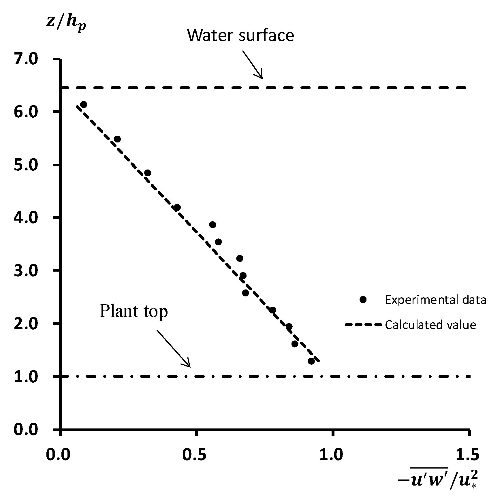
3.2. Second Order Turbulent Momentum

Figure 7 shows the vertical profile of the second order of turbulent momentum $-\overline{u^{\prime }{w}^{\prime }}$. Over the canopy, where $z/h_p\ge 1$, the value of $-\overline{u^{\prime }{w}^{\prime }}$ reaches a maximum value near the top of the plants, then varies upwards towards the water surface with elevation $z$ in a negative linear pattern. In general, this pattern agrees with other reports (e.g., [33]). This pattern implies that the dense plants can be considered as rough permeable bottom boundary for the over flow. The experimental data shows a good agreement with a plant-height modified linear formula, which was proposed by Nezu and Sanjou (2008) [22]:

$$-\overline{u^{\prime }{w}^{\prime }}=\frac{\left(H-z\right)}{\left(H-h_p\right)}{u}_{*}^2.$$

(7)

It should be noted that near the water surface, the calculated value of $-\overline{u^{\prime }{w}^{\prime }}$ from Equation (7) is smaller than the observed data. This is mainly because the fluctuation of the water surface enhances the turbulence, thereby increasing the corresponding turbulent momentum.

3.3. Derivation of Turbulent Diffusivity of Flow

Based on Equations (5) and (7), the turbulent momentum diffusion coefficient (${\epsilon }_m$) can be derived. Taking the derivative of $u$ with respect to $z$ in Equation (5), yields

$$\frac{du}{dz}=\frac{d}{dz}[\frac{u_{*}}{k}\ln (\frac{z-d}{z_0})],$$

(8)

or:

$$\frac{du}{dz}=\frac{u_{*}}{k}\frac{d}{dz}[\ln (\frac{z-d}{z_0})].$$

(9)

For the convenience of integration, Equation (9) can be re-written as:

$$\frac{du}{dz}=\frac{u_{*}}{k}\frac{d}{z_0\times d(\frac{z-d}{z_0})}[\ln (\frac{z-d}{z_0})].$$

(10)

Re-arranging the right hand of Equation (10) yields:

$$\frac{du}{dz}=\frac{u_{*}}{k}\frac{1}{z_0}\frac{1}{(\frac{z-d}{z_0})},$$

(11)

i.e.,

$$\frac{du}{dz}=\frac{u_{*}}{k}(\frac{1}{z-d}).$$

(12)

Substituting Equations (12) and (7) into ${\epsilon }_m\equiv -\overline{u^{\prime }{w}^{\prime }}/\frac{du}{dz}$ yields

$${\epsilon }_m=\frac{(H-z)}{(H-h_p)}{u}_{*}^2/[\frac{u_{*}}{k}(\frac{1}{z-d})],$$

(13)

i.e.,

$${\epsilon }_m=k{u}_{*}\left(z-d\right)\frac{\left(H-z\right)}{\left(H-h_p\right)}.$$

(14)

3.4. Equilibrium Equation between Turbulent Diffusion and Gravitational Settling of Fine Suspended Sediments

The net flux of suspended sediments per unit area of a plane parallel to flow bed is described by

$$F_{eddy}=-{\epsilon }_s\left(\frac{d{C}_s}{dz}\right)=-\beta {\epsilon }_m\left(\frac{d{C}_s}{dz}\right),$$

(15)

where $C_s$ is the volumetric concentration of fine sediments.

Substituting of Equation (14) for $k_m$ in Equation (15) yields

$$F_{eddy}=\frac{-\beta k{u}_{*}\left(z-d\right)\left(H-z\right)}{H-h_p}\times \frac{d{C}_s}{dz}.$$

(16)

The downward flux of suspended sediments per unit area due to gravity is described by

$$F_{gravity}=-C_s\times {\omega }_s.$$

(17)

In the dynamic equilibrium state, $F_{eddy}+F_{gravity}=0$, that is,

$$\frac{-\beta k{u}_{*}\left(z-d\right)\left(H-z\right)}{H-h_p}\times \frac{d{C}_s}{dz}-C_s\times {\omega }_s=0.$$

(18)

Re-arranging Equation (18) in term of $d{C}_s/C_s$ yields

$$\frac{d{C}_s}{C_s}=\frac{{\omega }_s\left(H-h_p\right)}{-\beta k{u}_{*}}\times \frac{1}{\left(z-d\right)\left(H-z\right)}dz,$$

(19)

i.e.,

$$\frac{d{C}_s}{C_s}=\frac{{\omega }_s\left(H-h_p\right)}{\beta k{u}_{*}}\times \frac{1}{\left(z-d\right)\left(z-H\right)}dz.$$

(20)

Integrating the left- and right- hand sides of Equation (20) yields

$$ln{C}_s=\frac{{\omega }_s}{\beta k{u}_{*}}\frac{\left(H-h_p\right)}{\left(H-d\right)}ln\left|\frac{z-H}{z-d}\right|+C.$$

(21)

Since $\left(z-H\right)<0$, and $\left(z-d\right)>0$ over the plants, Equation (21) can be re-written as

$$ln{C}_s=\frac{{\omega }_s}{\beta k{u}_{*}}\frac{\left(H-h_p\right)}{\left(H-d\right)}ln(\frac{H-z}{z-d})+C.$$

(22)

Choosing a reference concentration $C_a$ as the integrating constant $C$ as a boundary condition of Equation (22):

$$C=\frac{{\omega }_s}{\beta k{u}_{*}}\frac{\left(H-h_p\right)}{\left(H-d\right)}ln(\frac{H-a}{a-d}),$$

(23)

to make $C_s=C_a$ at the height level where $z=a$.

Substituting Equation (23) into Equation (22), and then solving Equation (22) yields

$$\frac{C_s}{C_a}={\left(\frac{H-z}{z-d}\times \frac{a-d}{H-a}\right)}^{\frac{{\omega }_s}{\beta k{u}_{*}}\times \frac{\left(H-h_p\right)}{\left(H-d\right)}}.$$

(24)

Equation (24) indicates that the concentration profile of fine suspended sediments is independent of the roughness height $z_0$, neither of the constant $C$ in the modified semi-logarithmic law of flow velocity expressed by Equation (5). Equation (24) also indicates that over dense plants, an equilibrium state of fine suspended sediments under the dynamic balance between turbulent diffusion and gravitational settling can be obtained.

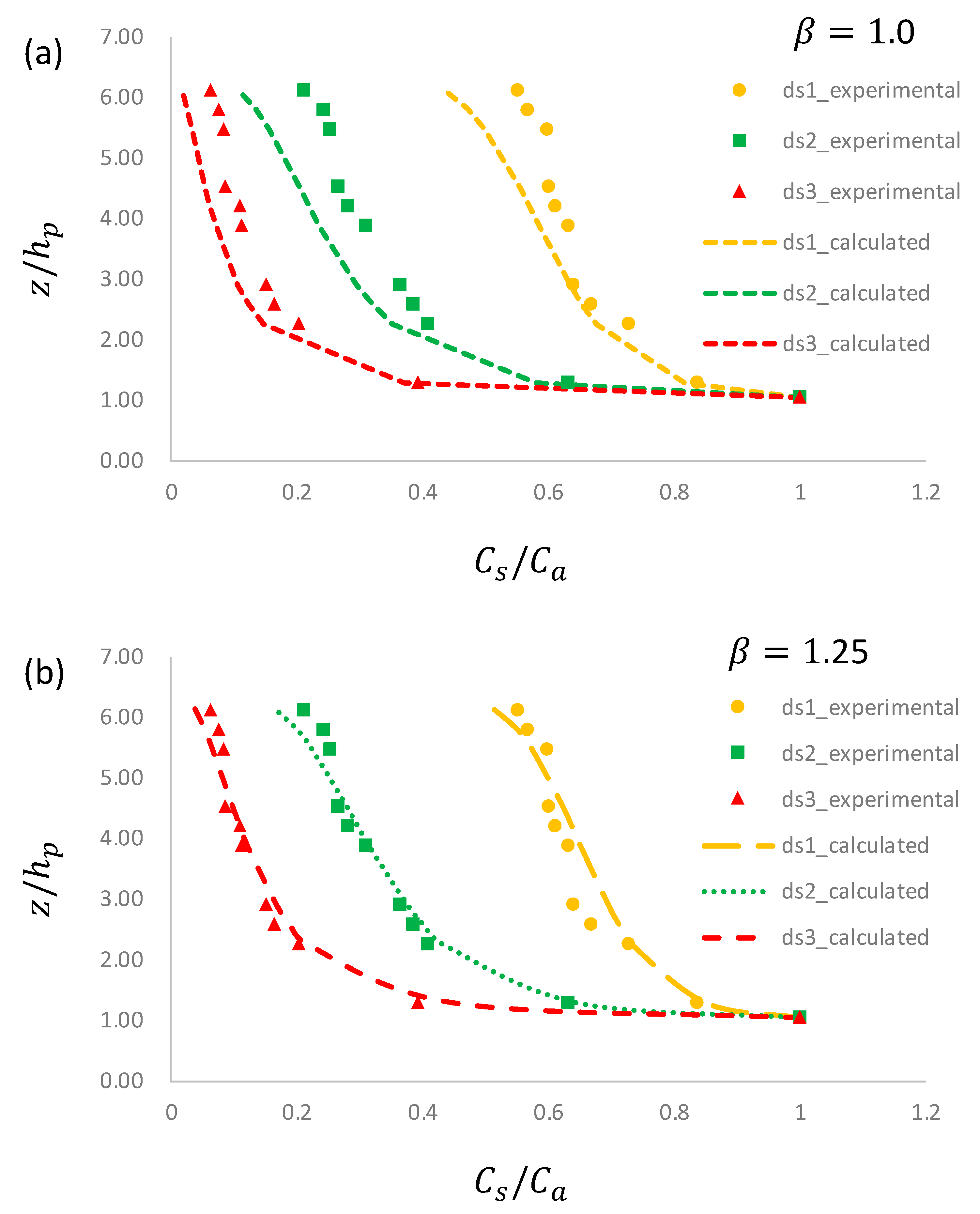
3.5. Experimental Results of the Profile of the Concentration of Suspended Sediments

Figure 8 shows the measured profile of the concentration of fine suspended sediments in the indoor physical experiments. Choosing the reference height $a=1.1h_p$, $\beta =1,$ and $\beta =1.25$, the calculated results of Equation (24) are plotted in Figure 8a,b. The comparison of Figure 8a,b show better agreement between calculated $C_s$ and the measured values for $\beta =1.25$ (Figure 8b).

Comparison between experiments using three diameters of suspended sediments is also shown in Figure 8b. For the smallest diameter (i.e., the least ${\omega }_s$), although the $C_a$-value was the smallest (Table 2), the $C_s/C_a$-value at all higher locations were the largest. For the largest diameter (i.e., the greatest ${\omega }_s$), the $C_a$ was the largest (Table 2), while the $C_s/C_a$-value at higher locations was the smallest. For the medium diameter, the concentrations at all height levels lay between the values for the smallest and largest diameters. This phenomenon indicates that given the same flow condition, the effect of turbulent diffusion on the suspension of fine sediments enhanced the decrease of settling velocity of sediment (${\omega }_s$), while the gravitational settling effect became weak with the decrease of ${\omega }_s$.

4. Discussion

The newly derived Rouse formula, which is modified by the zero-plane displacement ($d$) and the plant height ($h_p$) was validated by the observed profile of suspended sediment concentration ($C_s$) in the present study. This $d–h_p$ double modified Rouse formula is particularly suitable for describing dense plants with a high submergence ratio where the $d–h_p$ double modified logarithmic law of flow shear (Equation (5)) and the negative linear profile of shear turbulent momentum (Equation (7)) are applicable.

The Prandtl–Schmidt number ($\beta$) is influenced by different turbulence structures. In dense plant occupied flow, the characteristics of turbulence, including the turbulent kinetic energy, the skewed velocity and the intermittent features might have influence on the $\beta$-value. However, an accurate method for the determination of $\beta$-value has not been proposed. Therefore, it needs to be adjusted according to the conditions of the specified application.

In practical applications, the shear flow velocity $u_{*}$ can be estimated by the widely used plant-height modified Vanoni formula $u_{*}=\sqrt{gS\left(H-h_p\right)}$ [22,23,25,34,35]. For an after-flood flow, the suspended sediments in the above-plant region mainly come from the near-plant-top region, therefore a near-plant-top height level can be chosen for the reference $a$-value.

In applications, error in the estimation of $u_{*}$, $k$, $\beta$, ${\omega }_{\mathrm{s}}$, $h_p,$ or $d$ will lead to an error in suspension number, i.e., the exponent of the double-parameter modified Rouse formula Equation (24), and thus lead to an error in the estimation of the profile of suspended sediment concentration.

Some previous studies have attempted to make more complete model for the profile of suspended sediments [25]. However, for the dense plant occupied flow, which is usually presented in bio-restoration projects, turbulent diffusion is not the dominant factor for the vertical distribution of suspended sediments due to the direct interference and obstacle effect of plant foliage on sediment. In addition, the movement of sediment in the deep part of plant is limited within the plant foliage or tends to deposited on the flow bed by the retention effect of the plant foliage or roots. Therefore, separate investigation of the over-plant region is required.

5. Conclusions

A set of indoor experiments was conducted to investigate the vertical distribution of suspended sediments over dense plants in flowing water. The main conclusions are:

(1)

Over dense plants the velocity profile follows a semi-logarithmic law modified by $d$ and $z_0$. The second order turbulent momentum ($-\overline{u^{\prime }{w}^{\prime }}$) follows a negative linear function of $z$ and $\left(H-h_p\right)$. Based on these two laws, a new function of turbulent diffusion coefficient (${\epsilon }_m$) was derived.

(2)

Based on the dynamic balance between the upward turbulent diffusion and the downward gravitational settling, a $d–h_p$ double modified Rouse formula for the vertical distribution profile of fine suspended sediments was derived. The equation agrees well with experimentally observed data in the over-plant region.

(3)

With plants acting as a permeable bottom boundary of the flow over it, the fine sediments suspend or re-suspend from the top of the plants. In the above-plant region, the validation of the $d$–$h_p$ double-parameter modified Rouse formula indicates that turbulent diffusion controls the upward movement of sediment.

References

- Kleeberg, A.; Kohler, J.; Sukhodolova, T.; Sukhodolov, A. Effects of Aquatic Macrophytes on Organic Matter Deposition, Resuspension and Phosphorus Entrainment in a Lowland River. Freshw. Biol. 2010, 55, 326–345. [Google Scholar] [CrossRef]
- Liu, J.H.; Yang, S.L.; Zhu, Q.; Zhang, J. Controls on Suspended Sediment Concentration Profiles in the Shallow and Turbid Yangtze Estuary. Cont. Shelf Res. 2014, 90, 96–108. [Google Scholar] [CrossRef]
- Rahimi, H.R.; Tang, X.; Singh, P. Experimental and Numerical Study on Impact of Double Layer Vegetation in Open Channel Flows. J. Hydrol. Eng. 2019, 25, 04019064. [Google Scholar] [CrossRef]
- Tunçsiper, B. Combined Natural Wastewater Treatment Systems for Removal of Organic Matter and Phosphorus from Polluted Streams. J. Clean. Prod. 2019, 228, 1368–1376. [Google Scholar] [CrossRef]
- Alemu, T.; Bahrndorff, S.; Alemayehu, E.; Ambelu, A. Agricultural Sediment Reduction Using Natural Herbaceous Buffer Strips: A Case Study of the East African Highland. Water Environ. J. 2017, 31, 522–527. [Google Scholar] [CrossRef]
- Abdelhakeem, S.G.; Aboulroos, S.A.; Kamel, M.M. Performance of a Vertical Subsurface Flow Constructed Wetland under Different Operational Conditions. J. Adv. Res. 2016, 7, 803–814. [Google Scholar] [CrossRef] [Green Version]
- Leguédois, S.; Ellis, T.W.; Hairsine, P.B.; Tongway, D.J. Sediment Trapping by a Tree Belt: Processes and Consequences for Sediment Delivery. Hydrol. Process. 2008, 22, 3523–3534. [Google Scholar] [CrossRef]
- Wahab, M.A.A.; Maldonado, M.; Luter, H.M. Effects of Sediment Resuspension on the Larval Stage of the Model Sponge Carteriospongia foliascens. Sci. Total Environ. 2019, 695, 133837. [Google Scholar] [CrossRef] [Green Version]
- Reidenbach, M.A.; Timmerman, R. Interactive Effects of Seagrass and the Microphytobenthos on SedimentSuspension Within Shallow Coastal Bays. Estuaries Coasts 2019, 42, 2038–2053. [Google Scholar] [CrossRef]
- Nikora, V. Hydrodynamics of Aquatic Ecosystems: An Interface between Ecology, Biomechanics and Environmental Eluid Mechanics. River Res. Appl. 2010, 26, 367–384. [Google Scholar] [CrossRef]
- Nepf, H.M. Hydrodynamics of Vegetated Channels. J. Hydraul. Res. 2012, 50, 262–279. [Google Scholar] [CrossRef] [Green Version]
- Cheng, N.S.; Nguyen, H.T.; Tan, S.K.; Shao, S.D. Scaling of Velocity Profiles for Depth-Limited Open Channel Flows Over Simulated Rigid Vegetation. J. Hydraul. Eng. 2012, 138, 673–683. [Google Scholar] [CrossRef]
- Cheng, N.S. Single-Layer Model for Average Flow Velocity with Submerged Rigid Cylinders. J. Hydraul. Eng. 2015, 141, 06015012. [Google Scholar] [CrossRef]
- Stephan, U.; Gutknechtb, D. Hydraulic Resistance of Submerged Fexible Vegetation. J. Hydrol. 2002, 269, 27–43. [Google Scholar] [CrossRef]
- Kouwen, N.; Unny, T.E.; Hill, H.M. Flow Retardance in Vegetated Channels. J. Irrig. Drain. Div. 1969, 95, 329–340. [Google Scholar]
- Nnaji, S.; Wu, I. Flow Resistance from Cylindrical Roughness. J. Irrig. Drain. Div. 1973, 99, 15–26. [Google Scholar]
- El-Hakim, O.; Salama, M.M. Velocity Distribution inside and above Branched Fexible Roughness. J. Irrig. Drain. Eng. 1992, 118, 914–927. [Google Scholar] [CrossRef]
- Klopstra, D.; Barneveld, H.J.; van Noortwijk, J.M.; van Velzen, E.H. Analytical Model for Hydraulic Roughness of Submerged Vegetation. In Proceedings of the 27th IAHR Congress, San Francisco, CA, USA, 10–15 August 1997; pp. 775–780. [Google Scholar]
- Wang, X.Y.; Xie, W.M.; Zhang, D.; He, Q. Wave and Vegetation Effects on Fow and Suspended Sediment Characteristics: A Fume Study. Estuar. Coast. Shelf Sci. 2016, 182, 1–11. [Google Scholar] [CrossRef]
- Nepf, H.M.; Vivoni, E.R. Flow Structure in Depth-Limited, Vegetated Flow. J. Geophys. Res. Oceans 2000, 105, 28547–28557. [Google Scholar] [CrossRef]
- Ghisalberti, M.; Nepf, H.M. The Limited Growth of Vegetated Shear Layers. Water Resour. Res. 2004, 40, 1–12. [Google Scholar] [CrossRef]
- Nezu, I.; Sanjou, M. Turbulence Structure and Coherent Motion in Vegetated Canopy Open-channel Flows. J. Hydro-Environ. Res. 2008, 2, 62–90. [Google Scholar] [CrossRef]
- Li, D.; Yang, Z.; Sun, Z.; Huai, W.; Liu, J. Theoretical Model of Suspended Sediment Concentration in a Flow with Submerged Vegetation. Water 2018, 10, 1656. [Google Scholar] [CrossRef] [Green Version]
- Huai, W.; Yang, L.; Wang, W.J.; Guo, Y.; Wang, T.; Cheng, Y. Predicting the Vertical Low Suspended Sediment Concentration in Vegetated Flow Using a Random Displacement Model. J. Hydrol. 2019, 578, 124101. [Google Scholar] [CrossRef]
- Yang, W.; Choi, S.U. A Two-layer Approach for Depth-limited Open-channel Flows with Submerged Vegetation. J. Hydraul. Res. 2010, 48, 466–475. [Google Scholar] [CrossRef]
- Rouse, H. Modern Conceptions of the Mechanics of Fluid Turbulence. Trans. ASCE 1937, 102, 463–505. [Google Scholar]
- Fredsøe, J.; Deigaard, R. Mechanics of Coastal Sediment Transport; World Scientific: Singapore, 1992. [Google Scholar]
- Wooding, R.; Bradley, E.; Marshall, J. Drag due to regular arrays of roughness elements. Bound. Layer Meteorol. 1973, 5, 285–308. [Google Scholar] [CrossRef]
- Goring, D.G.; Nikora, V.I. Despiking acoustic doppler velocimeter data. J. Hydraul. Eng. 2002, 128, 117–126. [Google Scholar] [CrossRef] [Green Version]
- Cheng, C.; Song, Z.; Wang, Y.; Zhang, J. Parameterized Expressions for an Improved Rouse Equation. Int. J. Sedim. Res. 2013, 28, 523–534. [Google Scholar] [CrossRef]
- Bagnold, R.A. An Approach to the Sediment Transport Problem from General Physics; Geological Survey professional 422-I; USA Government Printing Office: Washington, DC, USA, 1966.
- van Rijn, L.C. Principles of Sediment Transport in Rivers, Estuaries and Coastal Seas; Aqua Publications: Amsterdam, The Netherlands, 1993. [Google Scholar]
- Afzalimehr, H.; Najfabadi, E.F.; Singh, V.P. Effect of Vegetation on Banks on Distributions of Velocity and Reynolds Stress under Accelerating Flow. J. Hydrol. Eng. 2010, 15, 708–713. [Google Scholar] [CrossRef]
- Murphy, E.; Ghisalberti, M.; Nepf, H. Model and Laboratory Study of Dispersion in Flows with Submerged Vegetation. Water Resour. Res. 2007, 43, W05438. [Google Scholar] [CrossRef]
- Yang, W.; Choi, S.U. Impact of Stem Flexibility on Mean Flow and Turbulence Structure in Open-channel Fows with Submerged Vegetation. J. Hydraul. Res. 2009, 47, 445–454. [Google Scholar] [CrossRef]
Figure 1.
Sketch of - modified velocity profile, where represents the water depth; represents the height of plant; represents the Karman constant; represents the shear flow velocity; represents the time-averaged flow velocity in streamwise direction; represents the vertical coordinate with upward direction positive; and represents the integration constant.
Figure 2.
Horizontal planar view of experimental setup.
Figure 3.
Side view of the experimental set up (not in scale).
Figure 4.
(a) Schematic of plant model and (b) staggered arrangement of plants.
Figure 5.
Height levels of seven sediment sampling bottles on two sets of rod.
Figure 6.
Semi-logarithmic law of flow velocity over a dense plant.
Figure 7.
Profile of the second order momentum of flow ().
Figure 8.
(a,b) Profile of for and 1.25.