A 2D Real-Time Flood Forecast Framework Based on a Hybrid Historical and Synthetic Runoff Database


Chair of Hydrology and River Basin Management, Department of Civil, Geo and Environmental Engineering, Technical University of Munich, Arcisstrasse 21, 80333 Munich, Germany
*
Authors to whom correspondence should be addressed.
Water 2020, 12(1), 114; https://doi.org/10.3390/w12010114
Submission received: 18 November 2019
/
Revised: 18 December 2019
/
Accepted: 24 December 2019
/
Published: 30 December 2019
(This article belongs to the Special Issue Recent Advances and New Directions in Flood Forecasting, Modeling, and Mapping)
Abstract
:Operational real-time flood forecast is often done on the prediction of discharges at specific gauges using hydrological models. Hydrodynamic models, which can produce inundation maps, are computationally demanding and often cannot be used directly for that purpose. The FloodEvac framework has been developed in order to enable 2D flood inundations map to be forecasted at real-time. The framework is based on a database of pre-recorded synthetic events. In this paper, the framework is improved by generating a database based on rescaled historical river discharge events. This historical database includes a wider variety of runoff curves, including non-Gaussian and multi-peak shapes that better reflect the characteristics and the behavior of the natural streams. Hence, a hybrid approach is proposed by joining the historical and the existing synthetic database. The increased number of scenarios in the hybrid database allows reliable predictions, thus improving the robustness and applicability of real-time flood forecasts.
1. Introduction
River flood events are a widespread problem that affect the lives of millions of people around the world. Flood damages, globally and in Europe, are characterized by a significant growing trend [1] that will probably increase even more in the future. Some studies project that in Europe floods with return periods over 100 years will double in frequency in the next 30 years with serious social and economic consequences on the environment, individuals, and communities [2]. At the same time, the increased availability of real-time remote sensing and spatially organized data, in addition to the traditional point gauges, can greatly improve the effectiveness of the flood management strategies [3,4] by implementing tools such as Early Warning Systems (EWS). EWSs are able to forecast flood events in real-time and issue warnings to the authorities or the population. They can also provide forecasts of the magnitude and extension of flood events and on the severity of possible damages, providing a valid and effective tool for practical emergency management. In order to prevent and mitigate casualties and economic losses, the EU Floods Directive clearly states that flood risk management plans should take into account flood forecasts and Early Warning Systems (EWS) built in a way that they are able to consider the characteristics of a river basin or sub-basin [5,6]. Thus, researchers and engineers have been extensively working on the development of cost-effective and rapid methods in the last decades [7].
Among the different approaches used to develop flood forecast tools are artificial neural networks [8,9], high-resolution precipitation radars [10,11,12], images and video footages of the water level [13,14], and atmospheric data [15,16]. Flood maps generated using 2D hydrodynamic models are one of the best tools for an efficient management strategy. Even though advances in high-computational models are available, they are not used operationally due to high infrastructure and maintenance costs associated with them; therefore, 2D models are usually too computationally demanding for providing real-time forecasts of an EWS. Even though 1D hydrodynamic models can be applicable for real-time forecasts, in the case of flooding, they lose representativeness because the flow is no longer contained in the 1D river cross-sections. Because of this, one of the most used approaches in the development of EWS consists in using databases containing a series of pre-recorded flood scenarios that can be easily and quickly accessed. Several methods based on this concept have been previously used for EWSs [17]. Most of them are based on 1D hydrodynamic models [17,18], and only a few of them make use of full 2D hydrodynamic simulations [19]. The main limitation of those studies is that the forecasts have a coarse spatial and temporal resolution. The vast majority associate the flood inundation extents to a single exceedance level, usually 100-year return period [5,20], or a limited number of scenarios [19].
A different approach, with a fine resolution and a wide range of discharge forecast, is presented by Bhola et al. (2018). The method is based on an offline database of high flow runoff curves and corresponding 2D inundation maps previously simulated with a fine spatial and temporal resolution. The offline flood maps are selected based on the forecasted discharge hydrographs in the gauges located upstream of the study area and the available simulations stored in the offline database. The term “offline” refers to maps retrieved from a pre-recorded database, as opposed to online which refers to maps produced at real-time [5]. In this paper, we focus on improving the runoff database by including scaled historical flow data series in order to provide a more robust hybrid database.
2. Methods
2.1. Framework for Real-Time Flood Forecast
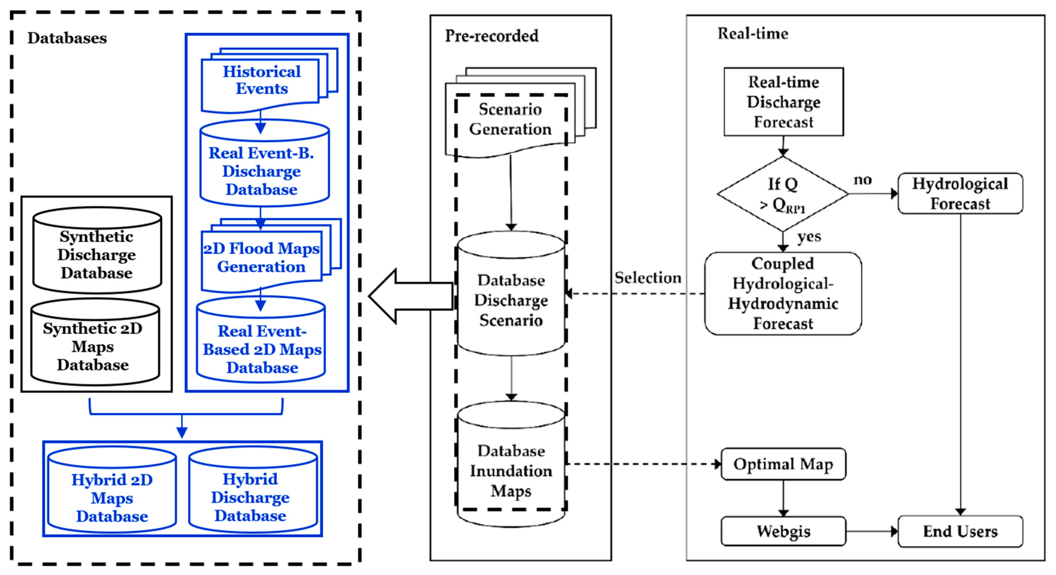
The forecast system is structured in an offline (pre-recorded) and an online (real-time) part. The offline part is composed of a database of discharge events linked to a database of corresponding 2D inundation maps (Figure 1). In order to produce the offline flood map database, the 2D hydrodynamic model HEC-RAS 2D, version 5.0.3 (Hydrologic Engineering Center-River Analysis System, Davis, CA, USA) was used. Each one of the runoff events stored in the offline database is used as inflow boundaries conditions of the 2D model. The model uses as boundary conditions only the flow of the three gauges while the rainfall on the catchment is neglected. This approach is based on the fact that the volume of direct precipitation, on the relatively small area of Kulmbach, is much less than the flow of the three gauges which collect the water from the larger catchments upstream. This means that, even in case of strong precipitation, the inflow into the river from the limited area of Kulmbach would be negligible in comparison to the total discharge of the river. Moreover, in case of flooding the water inside the area would flow away from the river into the land. This framework is thus designed for the prediction of river floods instead of pluvial. The high-resolution results for the water depth in each cell are stored with an interval of 15 min in the offline maps database. The online part provides the river discharge predictions of the hydrological model. If the predicted discharge values exceed a certain threshold (Qlimit) corresponding to the flow having a return period larger than 1 year, the forecast system is activated. Once the framework is activated, it compares the discharge forecast curves with the offline database for increasing intervals of 3 h. Hence, 4 different offline hydrographs are selected for the intervals of 3, 6, 9, and 12 h and the most likely offline inundation map for every 15 min interval is returned. The tool “FloodEvac” built on MATLAB R2018a (version 9.4.0.813654, 64 bit, MathWorks Inc., Natick, MA, USA) automatizes the entire process [21]. A detailed description of the framework can be found in Bhola et al. (2018) [22]. The offline discharge databases are described in detail in Section 2.3. In a machine with CPU Intel® Core™ i7-6700HQ 2.60 GHz it takes about 5 min to produce a forecast of 12 h into the future, mainly due to the considerable size of the high-quality flood maps.
2.2. Evaluation Metrics
The metrics used in the evaluations of the fit between the online and offline discharge curves are the Nash–Sutcliffe efficiency (NSE), defined in (1), and the weighted coefficient of determination (Wr2), defined in (2). They are the most common performance criteria used in hydrological modelling [23].
where
where N is the number of samples, O the forecast (online) discharge, P the discharge in the offline database, and b the gradient of the regression line. NSE varies from minus infinity to a maximum of 1. Wr2 ranges from a minimum of 0 to a maximum of 1. The fitting between two series is considered good if the values of NSE and Wr2 are close to one. The first parameter to be considered is the NSE: the event giving the best value over 0.85 is selected [5,23,24]. In case no NSE is found higher than 0.85 the event with the best Wr2 over 0.85 is used. If the second criterion also fails the discharge event from the database with the best NSE is used. The values are calculated every 3 h for intervals of 3, 6, 9, 12 h respectively.
The quantitative evaluation of the forecasted 2D flood inundation extents is based on two parameters: Fit Statistic F [5,25], defined in (3) and the Absolute Error e, defined in (4).
A0 is the overlap of flooded cells in the online and offline maps, Aoffline is the flooded area in the offline map, Aonline is the flooded area in the online map, dioffline is the water depth of the cell i in the offline map, dionline is the water depth of the cell i in the online map and nf is the number of flooded cells. The Fit statistic expresses the ratio of the total overlap of the flooded area between the online and offline maps, and it ranges from 0 to 1. The absolute error in meters provides an indicator on the error of the forecasted water depths. A cell is defined as flooded if the water depth is more than 0.10 m [26].
2.3. Offline Runoff Databases
2.3.1. Real Event-Based Database (REBD)
The Real Events-Based Database (REBD) is based on the discharge time-series from 1970 to 2017 on 15-min resolution for the three gauges of Kauendorf, Ködntiz, and Unternzettlitz, obtained from the Gewässerkundlicher Dienst Bayern website (gkd.bayern.de) [27]. From the synchronized raw time series, a step by step process was applied in order to isolate single runoff events which have a significant magnitude. A series of analysis on the peaks and on the gradient of the flow allowed us to obtain events which start with a strong increase in flow and stop when the runoff decrease enough in gradient and magnitude. Since the discharge time series include few extreme flood events, smaller events were added in order to reach a total number of 180 events. The objective was to rescale the events to higher return periods. The process developed is divided into normalization, rescaling, and generation phase. Normalization aims to obtain a real events “shape” database that can be easily re-scaled for any desired return-period discharge and duration. Rescaling aims to set the height of the highest peak between the three gauges to the value of one, while keeping the discharge of the other two gauges proportional to the highest. The duration of the event is resampled to 1000 timesteps. Generation aims to produce rescaled historical river discharge events with different return periods. For this, 60 normalized events are randomly selected and are resampled to a duration of 800 timesteps of 15 min each (200 h) and the discharge is rescaled with a maximum return period for the three gauges. The return periods are extrapolated from the historical runoff series of the gauges using a Peak Over Threshold method based on Gumbel generalized extreme value distributions. As such one gauge will have the assigned return period T for the peak, while the other two gauges will keep the proportion of the historical event. The latter gauges will have therefore a lower or equal return period. In this study, each event was rescaled three times for a maximum return period of 50, 100, and 150 years. The database includes 180 discharge events.
2.3.2. Synthetic Database (SD)
The advantage of the synthetic database is that it can be easily created using only values of return periods and durations for scaling an initial Gaussian shape. Hence, its creation is easier than building an historical database from the runoff time-series. The drawback is that this database could miss some characteristics of the natural runoff of the streams in the area. The synthetic events database is the same as in Bhola et al. (2018). It is built on a time-series of synthetic discharge shapes with different peak intensities and gradients. The synthetic events are based on the information on the probability of rainfall available from the Atlas distributed by the German Meteorological Services Deutscher Wetterdienst (DWD) KOSTRA (Koordinierte Starkniederschlags Regionalisierungs Auswertungen) [5,22]. The water balance model LARSIM (Large Area Runoff Simulation Model) was used to generate the inflow boundary conditions for the hydrodynamic 2D model in HEC-RAS using the produced rainfalls series [22]. The database includes 180 runoff events.
2.3.3. Hybrid Database (HD)
The hybrid database (HD) joins both the synthetic and the Real Event-Based databases. The HD is created by joining the two databases together in order to form a more complete database of 360 events.
2.4. Hydrodynamical Model
2.4.1. Main Equations
The HEC-RAS 2D solver is an implicit finite difference algorithm that discretizes the time derivatives and hybrid approximations by combining finite differences and finite volumes to discretize spatial derivatives [28]. The shallow water equations can be solved using the 2D Diffusion Wave computational method, derived from the full 2D Saint Venant Full Momentum equation, on the assumption that the inertial terms can be neglected [29]. The simplified set of equations, defined in (5), (6), (7), and (8), makes the simulation faster and numerically more stable even with wider time steps and spatial discretization.
H is the surface elevation (m), h is the water depth (m), u, v are the velocity components in the x- and y-direction (m/s), q is the source/sink term, g is the gravitational acceleration (m/s2), cf is the bottom friction coefficient (1/s), R is the hydraulic radius (m), |V| is the magnitude of the velocity vector (m/s), and n is the Manning’s roughness coefficient (s/m1/3)
2.4.2. Model and Boundary Conditions
The model covers an area of 11.5 km2 for a total of 430,485 cells, of which 193,161 are in the domain utilized for the forecasts. The average area of the cells is 24.8 m2, with a maximum of 59.8 and a minimum of 6.8 m2. The calibrated Manning’s coefficient used in the model [5] are shown in Table 1.
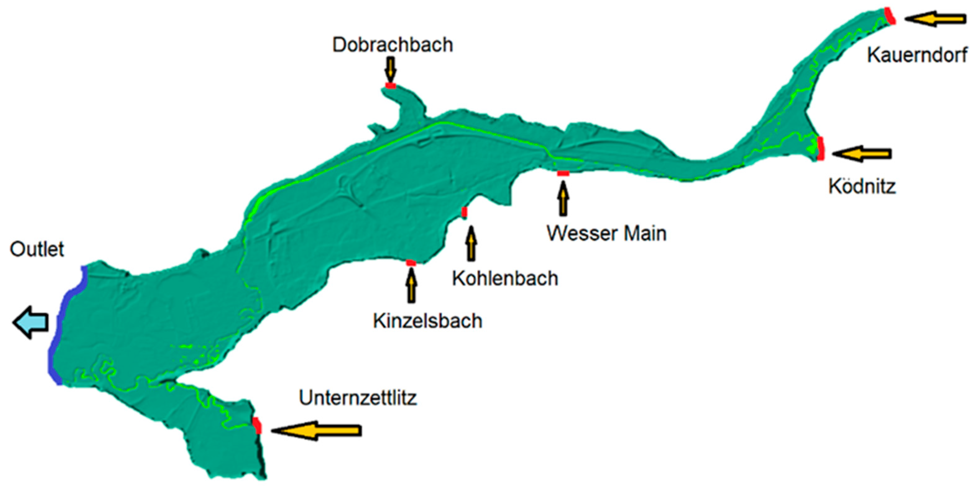
The boundary conditions set for the model are of three typologies: inflow hydrographs, no-flow boundaries, and normal depth. The hydrographs of each event contained in the databases are directly used as inflow boundary conditions. Secondary inflows are set by default to 5% of the flow rate of Ködntiz as their water contribution is scarce in comparison with the main streams. The north, east, and south borders of the area are set as no-flow boundaries, as the area itself is surrounded by hills which delineate the basin. The south-western border of the grid is set as an outlet with a normal depth boundary condition. Due to the topology and the significant slope of the area, it is highly unlikely that the flooding events from upstream occurring in Kulmbach would be affected by backwater from downstream.
3. Study Area and Data
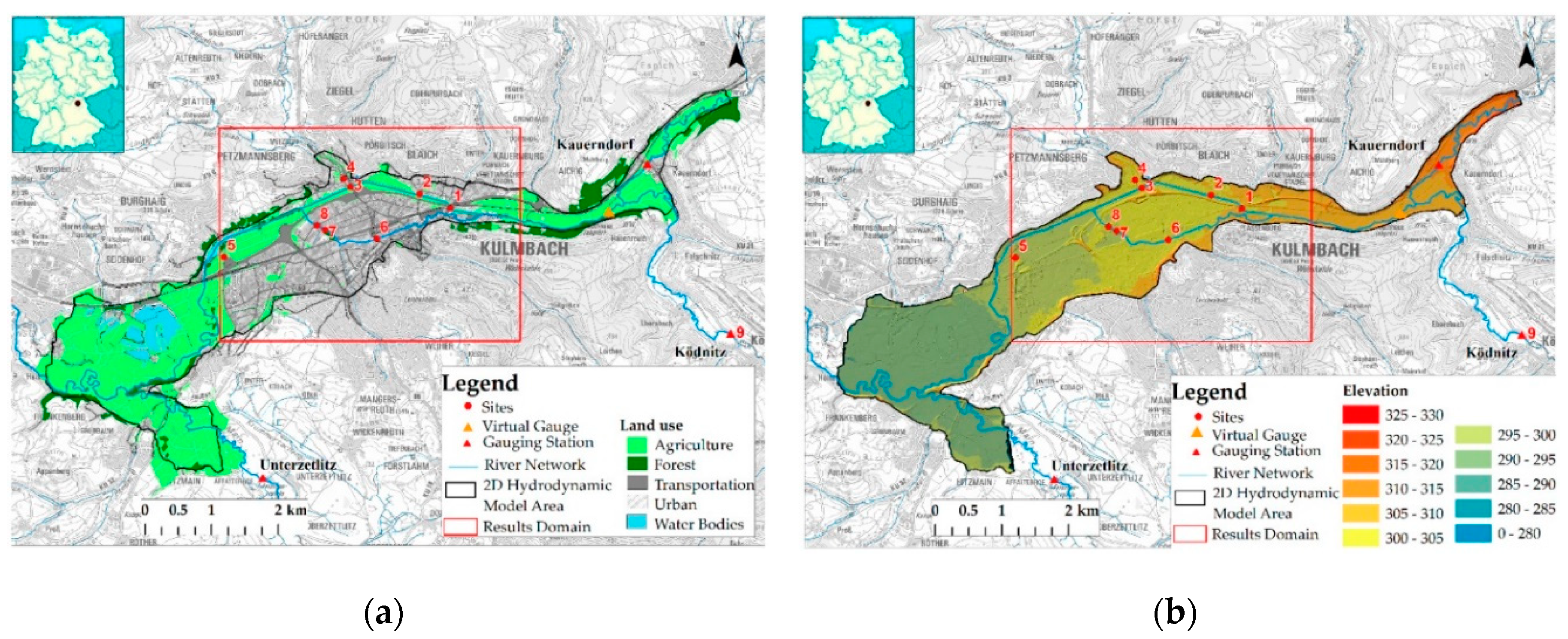
The site of the study was the area around the city of Kulmbach, in northern Bayern. The area has approximately 12 km2 and contains the city center (Figure 2). The water bodies (channel and lakes) account for 7%, the urban area covers 26%, including industrial and residential buildings and transport infrastructures as roads and railway tracks; forests account for 5% of the total area [5]. The area is elongated and narrow in the north-eastern part, with a fluvial valley surrounded by hills. In the eastern part, it widens as the valley enters a flood plain area. The town of Kulmbach is situated in the center of the area. The maximum elevation is located in the higher north-eastern part with 325 m, while the minimum is located in the lower south-eastern one with 290 m. The three main rivers entering the area are the Schorgast and the Weisser Main from north-east and the Rorter Main from the south-west. The discharge of the rivers is recorded at the gauge stations of Kauerndorf, Ködntiz, and Unternzettlitz respectively. Other minor streams are entering the area from the north (Dodrachbach) and south (Kinzelsbach, Kohlenbach), but their discharges can be neglected in comparison with the three main rivers. The outlet of the area is situated in the western part.
The historical runoff events extraction is carried out on the full discharge series from 1970 to 2017 for the three gauges of Kauerndorf, Ködntiz, and Unternzettlitz, obtained from the Gewässerkundlicher Dienst Bayern website (gkd.bayern.de) [27]. Once all 2D hydrodynamic simulations are complete, and their online flood maps are produced, the runoff series are used to test both the synthetic and real-based runoff databases and the respective offline flood maps. The comparison between the online maps of the validation events and the forecasted offline maps are used to assess the quality of the forecast and thus the performance of the databases SD, REBD, and HD.
4. Application of the FloodEvac Framework
Because of the lack of real observed flood extensions for validating the framework, another approach was used [5,26]. Inundation maps for four historical runoff events were generated from the 2D hydrodynamic model and used to validate the system. Those maps will be referred to as online in this study. In order to apply the FloodEvac Framework to this area, a virtual gauge is created where the streams coming from Kauerndorf and Ködntiz join. The discharge in this virtual gauge is assumed to be the sum of the flow of the two mentioned gauges. The flow of Unternzettlitz is neglected. The activating discharge value for the forecasting framework to start is set to the sum of the 1-year return period flows of the two gauges of Kauerndorf and Ködntiz, which is equal to 76 m3/s at the virtual gauge. The online and offline discharge curves at the virtual gauge are compared using NSE and Wr2 measures. As such the forecasts are valid only in the area between the virtual gauge in the east and the inflow at Unternzettlitz in the west as shown in the red square in the following Figure 3. Because the actual area of the forecast is smaller than the total area of the hydrodynamic model the predictions are robust against issues which may arise due to the settings of the boundary conditions in the model. The 2D hydrodynamic model HEC-RAS is applied to generate the maps of the databases. Details about the setup, calibration, and validation of HEC-RAS can be found in Bhola et al. (2018) and Bhola et al. (2019) [30].
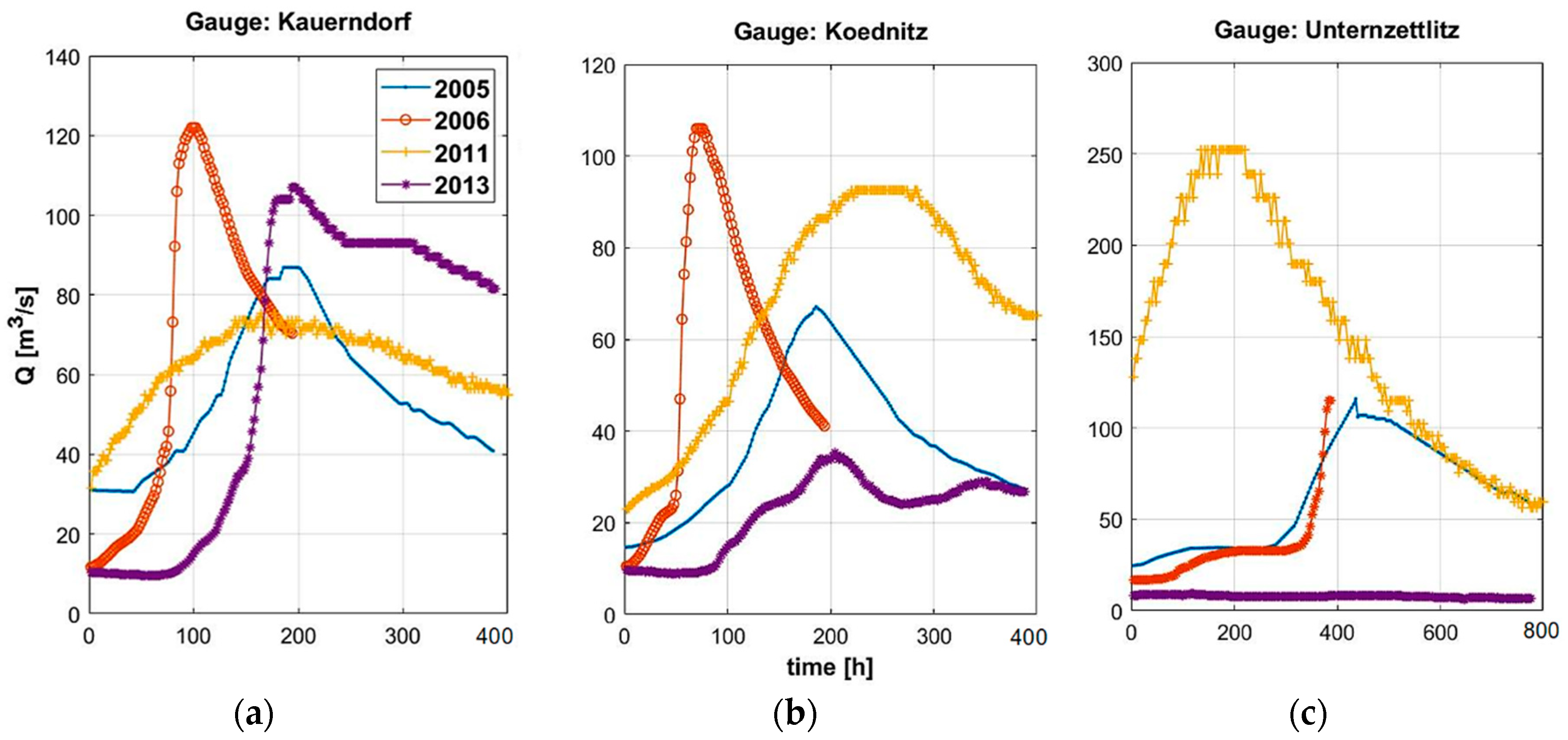
Four high flow runoff events are selected for the validation from the historical time series as shown in Figure 4. The events occurred in February 2005, May 2006, January 2011, and May 2013. It is important to note that those runoff events were not used in the production of the REBD and therefore they are not biased and can be used for the validation of the framework.
5. Results and Discussion
5.1. Databases
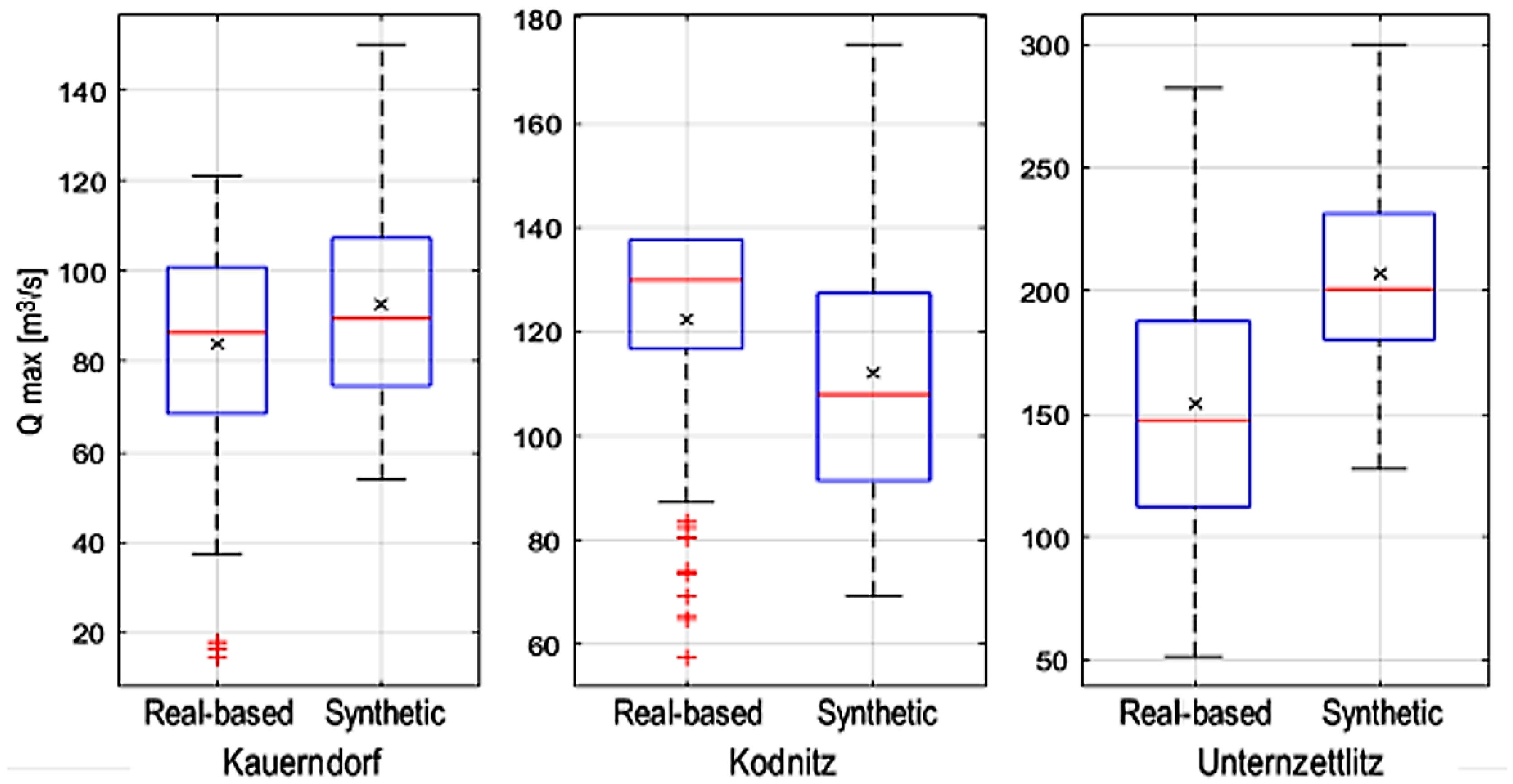
The distribution of the peak flow of the events in the REBD and SD are shown in Figure 5. The distribution of the maximum flow rate for the different gauges is in general different between the two databases and the gauges. While for Kauerndorf and Unternzettlitz the peaks are almost normally distributed for both the databases, for the gaugeof Ködnitz the REBD’s peaks are in average higher than the SD’s ones, with few low flow values. That is because REDB implicitly considers that Ködnitz is the most important gauge as it directly crosses Kulmbach and the runoff is higher than Kauerndorf, while the SD does not differentiate between the two.
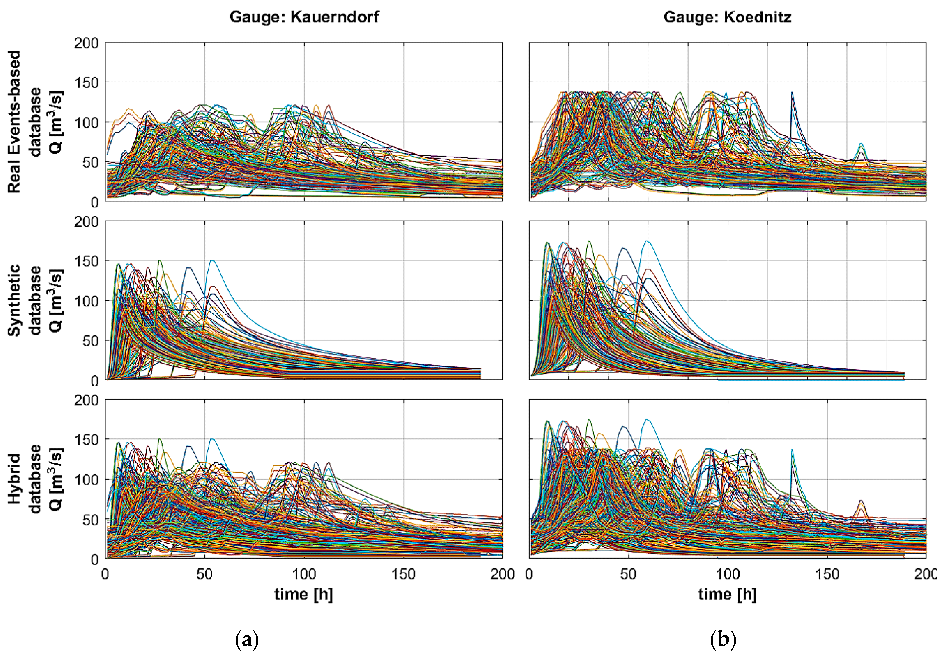
The REBD, obtained by the selection and rescaling of the historical events, the Synthetic Database SD and the Hybrid Database HD are plotted in Figure 6 for the two gauges of Kauerndorf and Ködntiz.
It is easy to notice the significant difference between the smooth, mono-peak shapes of the SD and the irregular curves of the REDB. The HD includes both databases. Another main difference between SD and REDB is the time of peaking of the different curves: REDB has a significant number of very late events with multiple peaks. It should be noted that REDB preservers the relative proportions between the historical flows of the gauges intact. Those are not bound by a linear or quasi-linear relation, but instead by the correlation between the Gumbel probability distributions which fit each flow data series. Since SD has been built based on synthetic events a quasi-linear relationship between the gauges can be observed (Figure 7).
For the REBD in the first and third scatter a high number of values are aligned with the discharge corresponding to the 50, 100, and 150 return period, while the SD shows a quasi-linear relation. Therefore, REDB preserves the proportion between the discharges at the three gauges for the extreme event as it takes into account also scenarios where only one or 2 gauges have a high return period.
Based on that it is possible to assume that the SD will have an advantage in fitting short and regular events for which the return period of the 2 gauges is similar. The use of REDB will be advantageous for longer and irregular events, and likely for forecasts longer than 12 h.
5.2. Database Validation
The forecast system is tested using the SD, REBD, and HD databases on four historical events: February 2005, May 2006, January 2011, and May 2013. The fit of the discharge series of each validation event is shown in Figure 8 for each database. The best fits are marked in different colors for the forecasted intervals of 3, 6, 9, and 12 h along with the validation discharge curve (red). The hydrographs of those validation events tend to be quite regular with only one smooth peak. While the events of 2005 and 2011 have a slower rise, 2006 and 2013 peaks quite fast. Those characteristics favor SD for 2006 and 2013, while for the other two years the performances seem to be quite similar between the three databases.
The results of the discharge series fitting using NSE and Wr2 as a goodness-of-fit criteria perform well for all databases for the validation events of 2005, 2011, 2013 (Figure 8). Regarding the case of 2006, Figure 8 b.2, the discharge peak occurs too soon. As such the REBD results are outperformed by the SD and the HD. The results of the selected best fitting discharge curve and the related NSE/Wr2 for the REDB, SD, and HD are shown for the four validation events of 2005, 2006, 2011, and 2013 in Table 2.
The NSE values for the REBD are between 0.90 and 0.99 for the events of 2005, 2011, and 2013, with the exception of a 0.7 NSE value obtained for the 12 h interval in 2013, in which even the second fit criteria Wr2 could not find one event in the database with a value larger than 0.85. The values for SD also vary between 0.90 and 0.99, with the exception of the value for the 12 h interval in 2013 where NSE is below 0.85. In this case, the second fit criteria were activated and an event with Wr2 equal to 0.87 was found. The REDB perform worst in the short and steep event of 2006 because the events in this database typically have longer durations.
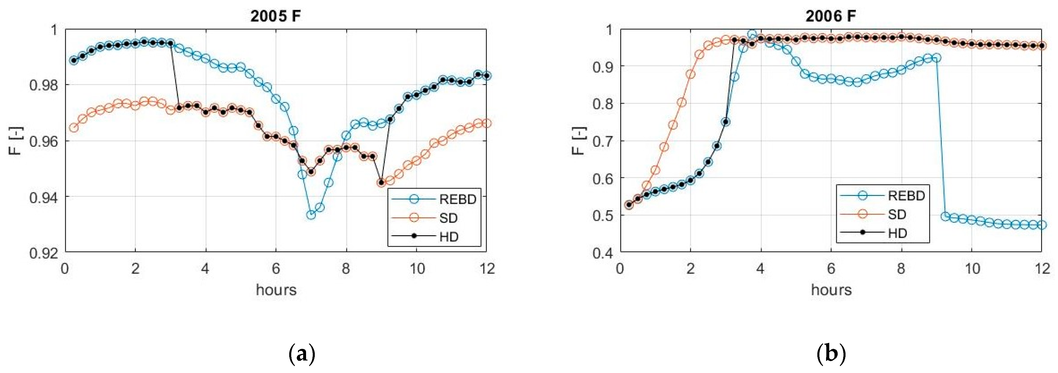
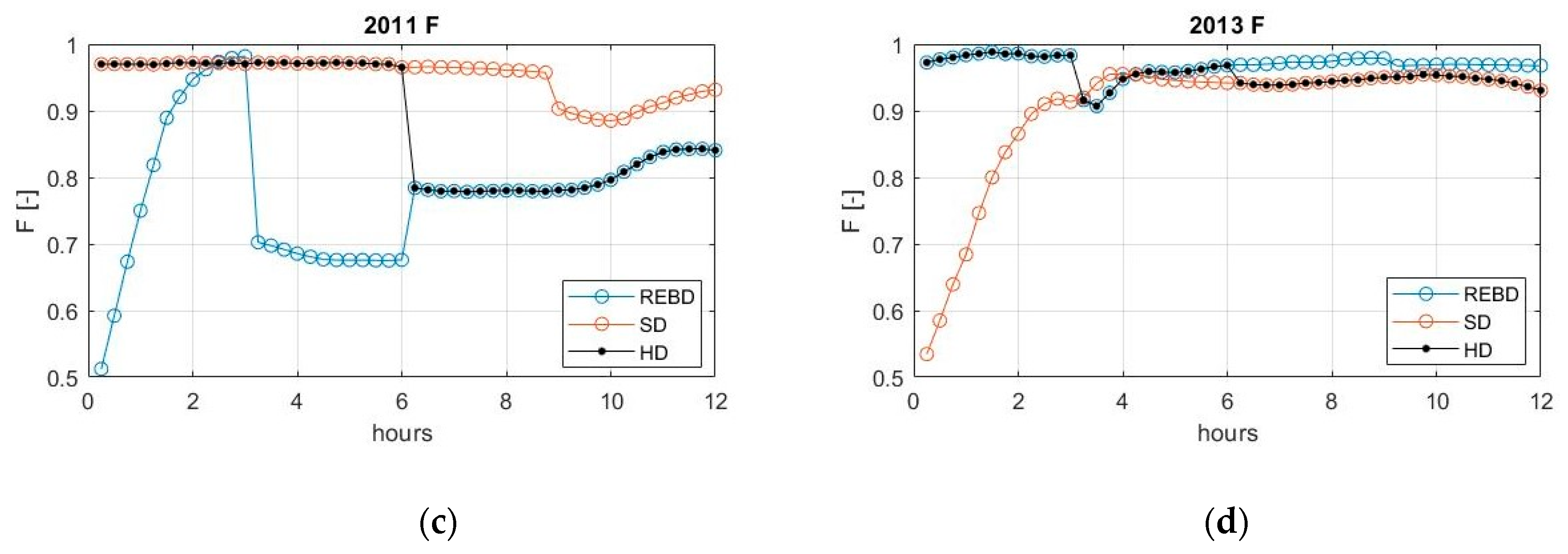
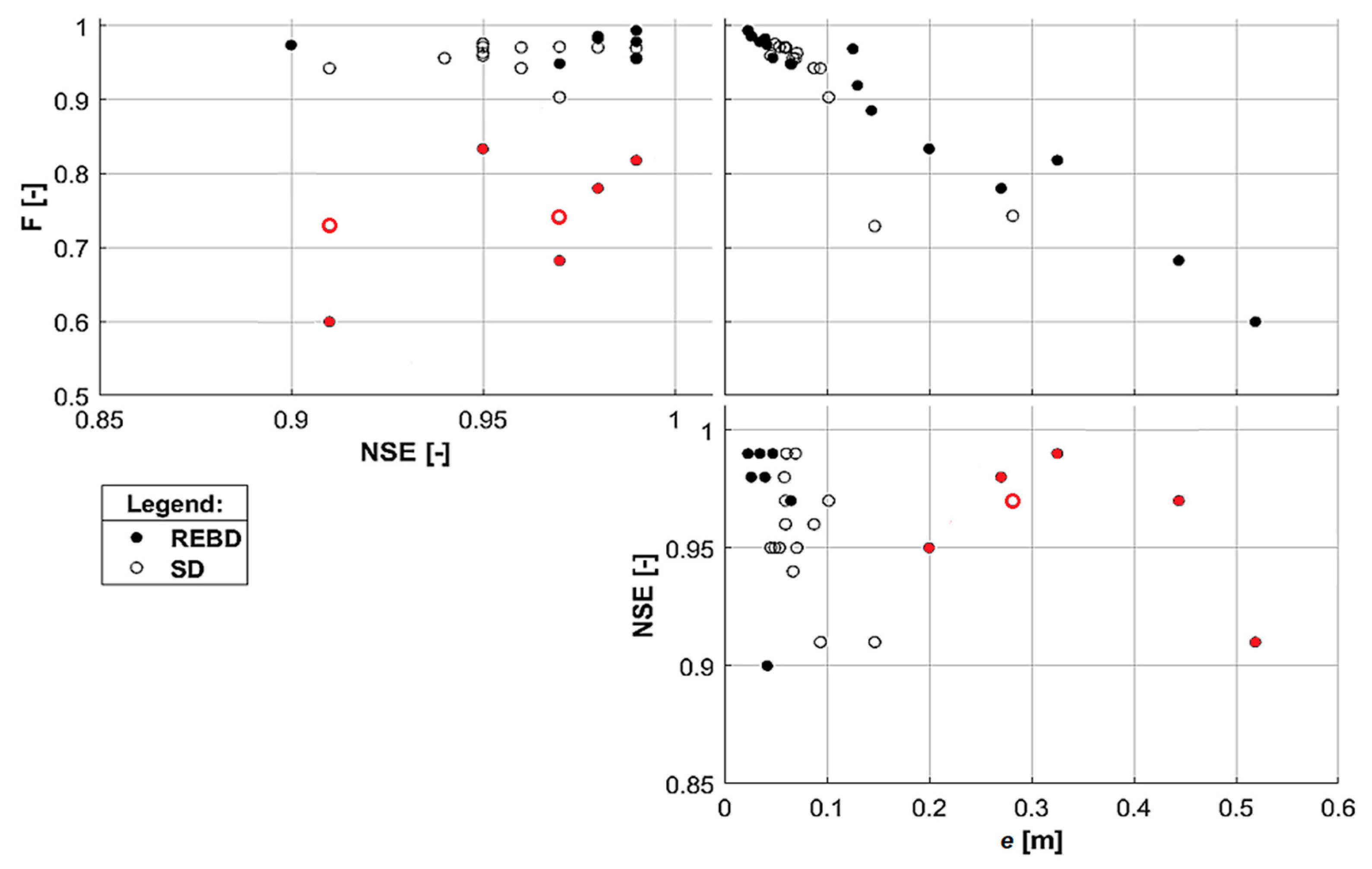
In Table 3, the average for the time intervals of 3, 6, 9, and 12 h of the comparison criteria for the online and offline flood maps FitStatistic and average absolute error in water depth is shown for each one of the validation events for REBD, SD, and HD. All three databases give satisfactory results: the average absolute error in water depth is usually between 0.03 and 0.3 m and the overlaps of the flooded area above 90% with the exception of REDB in 2006 and 2011. SD outperformed the REBD for the events of 2006 and 2011, while the REBD performed better in 2005 and 2013 regarding both e and FitStatistic parameters. HD always gives an average result in between the values of the two other databases. Figure 9 helps to explain this particular behavior of HD, and shows the values every 15 min of Fit Statistic for each one of the validation events for the REBD (blue), SD (red), and HD (black). Because HD is the ensemble of the two other databases, the result of HD are following either the pattern of SD or REBD for each 3 h interval as the best fit curve selected is either the best fit from SD or REDB, as can be clearly seen in Table 2. However, the best NSE score does not necessarily provide the best and e values between SD and REBD. The values of HD switch every 3 h to the values of SD or REBD, but that occurs according to the NSE value of the hydrograph; consequently, sometimes HD switch to the worst option in term of Fit Statistic. The same is valid also for e. The reason is that the NSE, the best-fit criteria for the runoff hydrographs at the virtual gauge, is not always well correlated with and e for values above 0.85. That is emphasized in the scatter plots in Figure 10, where the values of NSE above 0.85 are plotted against and e, and the values of and e against each other. In the first and third scatter it is obvious that poor values of and e can sometimes be obtained by very high values of NSE in the virtual gauge. As such, a quasi-linear correlation between the parameter is missing. That means that the NSE applied on the sum of Kauerndorf and Koednitz at the virtual gauge may be not the most effective way to select the hydrograph in the database that gives the best result as a flood map forecast. There could be several reasons for this; one possibility is that the virtual gauge summing both Kodnitz and Kauerndorf cannot take into account that different combination of discharges can have different impacts on the flooded area. In that respect, the separation of the two gauges could be more accurate. This solution would, however, require a substantial increase in the size of the database.
Overall, even though the best results are not always achieved by HD, the hybrid database guarantees more stability for the forecasts, meaning that the values of e and F outperform at least the worst of the two individual databases. The two smaller databases SD and REBD alone are more likely to encounter an event with characteristics one or the other cannot fit.
The framework is effective in forecasting flooding on the study area. The framework could be extended to forecast other 2D areas with similar size along a larger catchment. For larger 2D domains further consideration would need to be considered. Firstly, the number of the gauged input hydrographs may be considerably bigger and the location of these might create difficulties of using one single virtual gauge when the streams are entering the area from distant locations. This issue could be minimized by subdividing the area into smaller sub-catchments and applying the framework in each one. In this case, the hydrodynamic simulations could be run for each individual sub-area independently.
6. Conclusions
The FloodEvac framework for offline flood inundation forecast was extended to improve its performance by implementing different types of offline runoff databases. Previously, the framework included a database of synthetic rainfalls events with different return periods. In this study, a new concept of database which is built upon the historical time series of runoff gauges is presented. The aim was to include irregular multi-peaks shapes and simulate the realistic proportions between the flow in the three gauges. The two databases were joined in a single hybrid synthetic and historical database. The offline flood maps for the real events-based database were produced by running 180 2D hydrodynamic simulations. Together with the synthetic database, the joint database considered 360 events. The validation was carried out using four high flow events taken from the historical series which were not used in the production of the real events-based database. The validation was carried on a total duration of 12 h. Every 3 h the best-fit curve in the database and the relative offline flood maps every 15 min were selected and compared with the online maps simulated using the discharge curve of the validation event.
All three databases were tested with positive results. In most of the cases, the average absolute error in water depth was between 0.03 and 0.3 m and the overlaps of the flooded area above 90%. The database based on synthetic events was the one giving the best results in two cases out of four, while the one based on real events was more precise in the other two. The hybrid database had average results in between the two.
Overall, the use of a hybrid database instead of the individual ones can be considered advantageous, as it guarantees results with a better grade of reliability for a wider range of scenarios. The validation events used are Gaussian shaped but with a slight skewedness to the left and the forecasts were applied for a 12 h interval, so the earlier peaked and smoothed curves of the synthetic database were the ones giving (on average) the best results. For longer forecasts and more irregular hydrographs, the characteristics of the real based-database are expected to provide even more reliable result.
The increasing number of runoff scenarios including historical based shapes and a realistic proportion of the flow at the different gauges have a potential to gives reliable real-time flood maps and makes this forecast system a powerful tool for effective emergency management.
An important step in order to decrease the errors of the predictions would be to find a fit criteria between the offline and online hydrographs with a stronger correlation with the flood map errors. High values of NSE/Wr2 for the sum of the flow of Kauerndorf and Ködntiz at the virtual gauge are not correlated with the error in the flood maps, and that decrease greatly the ability of any database of giving the best flood map forecast. A solution could be to use a weighted coefficient (NSE or Wr2) for the two separate gauges of Ködntiz and Kauerndorf. That would take into account the proportion of the flow between the different stations overcoming the simplification of the virtual gauge.
Author Contributions
Conceptualization, J.L. and G.C.; Methodology J.L. and G.C..; Software, P.K.B. and G.C.; Validation, G.C.; Formal Analysis, G.C.; Investigation, G.C.; Resources, P.K.B. and J.L.; Data Curation, G.C. and P.K.B.; Writing-Original Draft Preparation, G.C.; Writing-Review & Editing, G.C., J.L. and P.K.B.; Visualization, G.C. and P.K.B.; Supervision, J.L. All authors have read and agreed to the published version of the manuscript.
Funding
This work was supported by the German Research Foundation (DFG) and the Technical University of Munich within the Open Access Publishing Funding Programme.
Acknowledgments
The authors would like to thank the Editors and anonymous Reviewers for their valuable and constructive comments related to this manuscript.
Conflicts of Interest
The authors declare no conflict of interest.
References
- Kundzewicz, Z.W.; Lugeri, N.; Dankers, R.; Hirabayashi, Y.; Döll, P.; Pińskwar, I.; Dysarz, T.; Hochrainer, S.; Matczak, P. Assessing river flood risk and adaptation in Europe-review of projections for the future. Mitig. Adapt. Strateg. Glob. Chang. 2010, 15, 641–656. [Google Scholar] [CrossRef]
- Alfieri, L.; Burek, P.; Feyen, L.; Forzieri, G. Global warming increases the frequency of river floods in Europe. Hydrol. Earth Syst. Sci. 2015, 19, 2247–2260. [Google Scholar] [CrossRef] [Green Version]
- Vojinovic, Z.; van Teeffelen, J. An integrated stormwater management approach for small islands in tropical climates. Urban Water J. 2007, 4, 211–231. [Google Scholar] [CrossRef]
- Price, R.K.; Vojinovic, Z. Urban flood disaster management. Urban Water J. 2008, 5, 259–276. [Google Scholar] [CrossRef]
- Bhola, P.; Leandro, J.; Disse, M. Framework for Offline Flood Inundation Forecasts for Two-Dimensional Hydrodynamic Models. Geosciences 2018, 8, 346. [Google Scholar] [CrossRef] [Green Version]
- UNISDR. Stormwater Management Handbook. Int. J. Eng. Technol. 2014, 2, 44. [Google Scholar]
- Bhatt, C.M.; Rao, G.S.; Diwakar, P.G.; Dadhwal, V.K. Development of flood inundation extent libraries over a range of potential flood levels: A practical framework for quick flood response. Geomat. Nat. Hazards Risk 2017, 8, 384–401. [Google Scholar] [CrossRef] [Green Version]
- Kim, G.; Barros, A.P. Quantitative flood forecasting using multisensor data and neural networks. J. Hydrol. 2001, 246, 45–62. [Google Scholar] [CrossRef]
- Campolo, M.; Soldati, A.; Andreussi, P. Artificial neural network approach to flood forecasting in the River Arno. Hydrol. Sci. J. 2003, 48, 381–398. [Google Scholar] [CrossRef]
- Pedersen, L.; Jensen, N.E.; Madsen, H. Calibration of Local Area Weather Radar-Identifying significant factors affecting the calibration. Atmos. Res. 2010, 97, 129–143. [Google Scholar] [CrossRef]
- Molina, L.S.T.; Harmsen, E.W.; Cruz-Pol, S. Flood alert system using rainfall forecast data in Western Puerto Rico. In Proceedings of the 2013 IEEE International Geoscience and Remote Sensing Symposium—IGARSS, Melbourne, VIC, Australia, 21–26 July 2013; pp. 574–577. [Google Scholar]
- Acosta-Coll, M. Low-Cost Weather Radars For Precipitation Detection And Development Of Air Operations In Colombia. Rev. Colomb. Tecnol. Adv. 2013, 2–22, 1692–7257. [Google Scholar]
- Bhola, P.K.; Nair, B.B.; Leandro, J.; Rao, S.N.; Disse, M. Flood inundation forecasts using validation data generated with the assistance of computer vision. J. Hydroinformatics 2019, 21, 240–256. [Google Scholar] [CrossRef] [Green Version]
- Acosta-Coll, M.; Ballester-Merelo, F.; Martinez-Peiró, M.; de la Hoz-Franco, E. Real-time early warning system design for pluvial flash floods—A review. Sensors (Switzerland) 2018, 18, 2255. [Google Scholar] [CrossRef] [Green Version]
- Cama-Pinto, A.; Acosta-Coll, M.; Piñeres-Espitia, G.; Caicedo-Ortiz, J.; Zamora-Musa, R.; Sepulveda-Ojeda, J. Diseño de una red de sensores inalámbricos para la monitorización de inundaciones repentinas en la ciudad de Barranquilla, Colombia. Ingeniare. Rev. Chil. Ing. 2016, 24, 581–599. [Google Scholar] [CrossRef] [Green Version]
- Ramírez-Cerpa, E.; Acosta-Coll, M.; Vélez-Zapata, J. Análisis de condiciones climatológicas de precipitaciones de corto plazo en zonas urbanas: Caso de estudio Barranquilla, Colombia. Idesia (Arica) 2017, 35, 87–94. [Google Scholar] [CrossRef]
- Hénonin, J. Urban flood real-time forecasting and modelling: A state-of-the-art review. In Proceedings of the DHI Conference, Kastrup, Denmark, 6–7 September 2010; p. 21. [Google Scholar]
- Henonin, J.; Russo, B.; Mark, O.; Gourbesville, P. Real-time urban flood forecasting and modelling-a state of the art. J. Hydroinformatics 2013, 15, 717–736. [Google Scholar] [CrossRef]
- Raymond, M.; Peyron, N.; Bahl, M.; Martin, A.; Alfonsi, F. ESPADA: Un outil innovant pour la gestion en temps réel des crues urbaines. In Proceedings of the 6th Novatech 2007—Sustainable Techniques and Strategies in Urban Water Management, Lyon, France, 25–28 June 2007. [Google Scholar]
- Dottori, F.; Kalas, M.; Salamon, P.; Bianchi, A.; Alfieri, L.; Feyen, L. An operational procedure for rapid flood risk assessment in Europe. Nat. Hazards Earth Syst. Sci. 2017, 17, 1111–1126. [Google Scholar] [CrossRef] [Green Version]
- Leandro, J.; Konnerth, I.; Bhola, P.; Amin, K.; Köck, F.; Disse, M. Floodevac Interface zur Hochwassersimulation mit Integrierten Unsicherheitsabschätzungen; Tag der Hydrologie–Forum für Hydrologie und Wasserbewirtschaftung: Trier, Germany, 2017; pp. 185–192. [Google Scholar]
- Bhola, P.; Leandro, J.; Konnerth, I.; Amin, K.; Disse, M. Dynamic Flood Inundation Forecast for the City of Kulmbach Using Offline Two-Dimensional Hydrodynamic Models. In Proceedings of the HIC 2018 13th International Conference on Hydrodynamics, Wuxi, China, 20 September 2018; Volume 3, pp. 258–265. [Google Scholar]
- Krause, P.; Boyle, D.P.; Bäse, F. Comparison of different efficiency criteria for hydrological model assessment. Adv. Geosci. 2005, 5, 89–97. [Google Scholar] [CrossRef] [Green Version]
- Moriasi, D.N.; Arnold, J.G.; van Liew, M.W.; Bingner, R.L.; Harmel, R.D.; Veith, T.L. Model evaluation guidelines for systematic quantification of accuracy in watershed simulations. Trans. ASABE 2007, 50, 885–900. [Google Scholar] [CrossRef]
- Quirogaa, V.M.; Kurea, S.; Udoa, K.; Manoa, A. Application of 2D numerical simulation for the analysis of the February 2014 Bolivian Amazonia flood: Application of the new HEC-RAS version 5. Ribagua 2016, 3, 25–33. [Google Scholar] [CrossRef] [Green Version]
- Leandro, J.; Djordjević, S.; Chen, A.S.; Savić, D.A.; Stanić, M. Calibration of a 1D/1D urban flood model using 1D/2D model results in the absence of field data. Water Sci. Technol. 2011, 64, 1016–1024. [Google Scholar] [CrossRef] [PubMed] [Green Version]
- Bavarian Environmental Agency. GKD Bayern. Available online: https://www.gkd.bayern.de/en/9 (accessed on 10 April 2019).
- HEC-RAS River Analysis System—Hydraulic Reference Manual, Version 5.0; USACE: Davis, CA, USA, 2016.
- Leandro, J.; Chen, A.S.; Schumann, A. Accepted Manuscript A 2D Parallel Diffusive Wave Model for floodplain inundation with variable time step (P-DWave) A 2D Parallel Diffusive Wave Model for floodplain inundation with variable time step (P-DWave) 1. J. Hydrol. 2014, 517, 38–39. [Google Scholar] [CrossRef]
- Bhola, P.K.; Leandro, J.; Disse, M. Reducing uncertainties in flood inundation outputs of a two-dimensional hydrodynamic model by constraining roughness. Nat. Hazards Earth Syst. Sci. 2019, 19, 1445–1457. [Google Scholar] [CrossRef] [Green Version]
Figure 1.
Framework of the offline flood inundation forecast including the pre-recorded and real-time extended from Bhola et al. (2018). The contributions presented in this paper are marked in blue.
Figure 1.
Framework of the offline flood inundation forecast including the pre-recorded and real-time extended from Bhola et al. (2018). The contributions presented in this paper are marked in blue.

Figure 2.
Model grid area with marked Inflows(red) and outflows (blue) boundary conditions.

Figure 3.
Land Use (a) and Terrain elevation (b) of the study area around Kulmbach from Bhola et al. (2018).
Figure 3.
Land Use (a) and Terrain elevation (b) of the study area around Kulmbach from Bhola et al. (2018).

Figure 4.
The four runoff events, February 2005, May 2006, January 2011, May 2013, selected for the validation plotted for the three gauges of (a) Kauerndorf, (b) Ködntiz and (c) Unternzettlitz.
Figure 4.
The four runoff events, February 2005, May 2006, January 2011, May 2013, selected for the validation plotted for the three gauges of (a) Kauerndorf, (b) Ködntiz and (c) Unternzettlitz.

Figure 5.
Comparison between the maximum flow of the three gauges for the events of the REBD and the SD.
Figure 5.
Comparison between the maximum flow of the three gauges for the events of the REBD and the SD.

Figure 6.
All the discharge events in the REBD, SD, and HD databases for the gauges of Kauerndorf (a) and Ködntiz (b).
Figure 6.
All the discharge events in the REBD, SD, and HD databases for the gauges of Kauerndorf (a) and Ködntiz (b).

Figure 7.
Scatter of the three river gauges plotted against each other for the maximum discharge for each event in the SD and REBD.
Figure 7.
Scatter of the three river gauges plotted against each other for the maximum discharge for each event in the SD and REBD.

Figure 8.
Comparison of runoff hydrographs at the virtual gauge for the event of May 2013 for SD (a), REBD (b), HD (c). The yellow lines represent the hydrographs of the offline database, the red line the runoff forecast, the light blue, blue, green, and black lines represent the selected offline hydrograph for the intervals of 3, 6, 9, and 12 h, respectively.


Figure 9.
Fit Statistic values every 15 min for the online and offline maps related to the four validation events of 2005 (a), 2006 (b), 2011 (c), and 2013 (d) using the REBD, SD, and HD.
Figure 9.
Fit Statistic values every 15 min for the online and offline maps related to the four validation events of 2005 (a), 2006 (b), 2011 (c), and 2013 (d) using the REBD, SD, and HD.


Figure 10.
Scatter plot of the good fit criteria for the runoff series NSE and the comparison criteria for the online and offline flood maps Fit Statistic F and average absolute error in water depth e. The exceptions with high NSE values but poor F and e performances are marked in red.
Figure 10.
Scatter plot of the good fit criteria for the runoff series NSE and the comparison criteria for the online and offline flood maps Fit Statistic F and average absolute error in water depth e. The exceptions with high NSE values but poor F and e performances are marked in red.


Table 1.
Calibrated Manning’s coefficient for the hydrodynamic model.
| Surface | Manning’s n (s/m1/3) |
|---|---|
| Water bodies | 0.022 |
| Crops and fields | 0.043 |
| Forests | 0.189 |
| Main roads | 0.014 |
| Urban area | 0.074 |
Table 2.
NSE/Wr2 goodness of fit and index of the selected event from the REBD, SD, and HD for the four validation events of 2005, 2006, 2011, and 2013.
Table 2.
NSE/Wr2 goodness of fit and index of the selected event from the REBD, SD, and HD for the four validation events of 2005, 2006, 2011, and 2013.
| Event | Interval (h) | REBD | SD | HD | |||
|---|---|---|---|---|---|---|---|
| Ev. Index | NSE/Wr2 (-) | Ev. Index | NSE/Wr2 (-) | Ev. Index | NSE/Wr2 (-) | ||
| 2005 | 3 | 180 | 0.99 | 9 | 0.98 | 180_R | 0.99 |
| 6 | 73 | 0.98 | 6 | 0.99 | 6_S | 0.99 | |
| 9 | 14 | 0.99 | 6 | 0.99 | 6_S | 0.99 | |
| 12 | 14 | 0.99 | 67 | 0.94 | 14_R | 0.99 | |
| 2006 | 3 | 51 | 0.91 | 135 | 0.91 | 51_R | 0.91 |
| 6 | 87 | 0.70 | 173 | 0.95 | 173_S | 0.95 | |
| 9 | 87 | 0.54 | 173 | 0.95 | 173_S | 0.95 | |
| 12 | 157 | 0.05 | 173 | 0.95 | 173_S | 0.95 | |
| 2011 | 3 | 83 | 0.95 | 10 | 0.96 | 10_S | 0.96 |
| 6 | 76 | 0.97 | 10 | 0.97 | 10_S | 0.97 | |
| 9 | 172 | 0.98 | 14 | 0.95 | 172_R | 0.98 | |
| 12 | 172 | 0.99 | 10 | 0.97 | 172_R | 0.99 | |
| 2013 | 3 | 41 | 0.98 | 115 | 0.97 | 41_R | 0.98 |
| 6 | 141 | 0.97 | 150 | 0.96 | 141_R | 0.97 | |
| 9 | 141 | 0.90 | 120 | 0.91 | 120_S | 0.91 | |
| 12 | 49 | 0.69 | 95 | 0.87 * | 95_S | 0.87 * | |
* The value refers to the Wr2 coefficient, as the NSE reached was below 0.85.
Table 3.
Average Fitstatistic and absolute error for each time interval using the three databases REBD, SD, and HD for the validation events of 2005, 2006, 2011, and 2013.
Table 3.
Average Fitstatistic and absolute error for each time interval using the three databases REBD, SD, and HD for the validation events of 2005, 2006, 2011, and 2013.
| F and e | 2005 | 2006 | 2011 | 2013 | |||||||||
|---|---|---|---|---|---|---|---|---|---|---|---|---|---|
| REBD | SD | HD | REBD | SD | HD | REBD | SD | HD | REBD | SD | HD | ||
| F (-) | 3 h | 0.99 | 0.97 | 0.99 | 0.60 | 0.77 | 0.60 | 0.83 | 0.97 | 0.97 | 0.98 | 0.78 | 0.98 |
| 6 h | 0.99 | 0.97 | 0.97 | 0.92 | 0.97 | 0.97 | 0.68 | 0.97 | 0.97 | 0.95 | 0.95 | 0.95 | |
| 9 h | 0.96 | 0.95 | 0.95 | 0.89 | 0.98 | 0.98 | 0.78 | 0.96 | 0.78 | 0.97 | 0.94 | 0.94 | |
| 12 h | 0.98 | 0.96 | 0.98 | 0.48 | 0.96 | 0.96 | 0.82 | 0.91 | 0.82 | 0.97 | 0.95 | 0.95 | |
| e (m) | 3 h | 0.02 | 0.06 | 0.02 | 0.52 | 0.13 | 0.52 | 0.20 | 0.06 | 0.06 | 0.04 | 0.26 | 0.04 |
| 6 h | 0.03 | 0.06 | 0.06 | 0.13 | 0.05 | 0.05 | 0.44 | 0.06 | 0.06 | 0.06 | 0.08 | 0.06 | |
| 9 h | 0.05 | 0.07 | 0.07 | 0.14 | 0.05 | 0.05 | 0.27 | 0.07 | 0.27 | 0.04 | 0.09 | 0.09 | |
| 12 h | 0.03 | 0.06 | 0.03 | 0.55 | 0.05 | 0.05 | 0.33 | 0.10 | 0.33 | 0.13 | 0.06 | 0.06 | |
© 2019 by the authors. Licensee MDPI, Basel, Switzerland. This article is an open access article distributed under the terms and conditions of the Creative Commons Attribution (CC BY) license (http://creativecommons.org/licenses/by/4.0/).
Share and Cite
MDPI and ACS Style
Crotti, G.; Leandro, J.; Bhola, P.K. A 2D Real-Time Flood Forecast Framework Based on a Hybrid Historical and Synthetic Runoff Database. Water 2020, 12, 114. https://doi.org/10.3390/w12010114
AMA Style
Crotti G, Leandro J, Bhola PK. A 2D Real-Time Flood Forecast Framework Based on a Hybrid Historical and Synthetic Runoff Database. Water. 2020; 12(1):114. https://doi.org/10.3390/w12010114
Chicago/Turabian StyleCrotti, Giampaolo, Jorge Leandro, and Punit Kumar Bhola. 2020. "A 2D Real-Time Flood Forecast Framework Based on a Hybrid Historical and Synthetic Runoff Database" Water 12, no. 1: 114. https://doi.org/10.3390/w12010114
Note that from the first issue of 2016, this journal uses article numbers instead of page numbers. See further details here.