Encounter Probability and Risk of Flood and Drought under Future Climate Change in the Two Tributaries of the Rao River Basin, China

Abstract

Extreme hydrometeorological events have far-reaching impacts on our daily life and may occur more frequently with rising global temperatures. The probability of the concurrence of these extreme events in the upper reaches of the river network is of particular importance for the lower reaches, which is referred to as the encounter probability of extreme events, and may have even stronger socio-economic impacts. In this study, the Rao River basin in China is selected as an example to explore the encounter probability and risk of future flood and drought based on the encounter probability model. The reference period was 1971–2000, and the future prediction periods were 2020–2049 and 2070–2099. The calibrated and validated statistical downscaling model (SDSM) was used to generate future daily precipitation and daily mean temperature. The calibrated and validated Xin’anjiang model was used to predict future daily mean streamflow in the basin. In addition, the encounter probability model was established using the joint distribution of occurrence dates and magnitudes of daily mean streamflow to investigate the encounter probabilities of flood and drought under future climate change. Results show that, for flood occurrence dates, the encounter probability during the flood season would decrease in the two future periods while the dates would generally be earlier. For flood magnitudes, the encounter probability of the two tributaries’ floods and the probability of flood at each tributary would decrease (e.g., the encounter probability with the same-frequency of 100-years would reduce by 53% to 95%), which indicates reduced risk of future major floods in the study area. For drought occurrence dates, the encounter probability during the non-flood season would decrease. For drought magnitudes, the encounter probability would decrease (e.g., the encounter probability with the same-frequency of 100-years would reduce by 18% to 33%), even though the probability of future drought at each tributary would increase. Such analyses provide important probabilistic information to help us prepare for the upcoming extreme events.

1. Introduction

Global climate change accelerates the processes of the global and regional hydrological cycle, which alters the spatial and temporal distribution of hydrological events such as precipitation, evaporation, and runoff. Consequently, water resources may be redistributed in time and space, which increases the occurrence probability of extreme hydrological events [1,2]. The probability of future extreme hydrological events has recently become a significant concern in climate change research [3,4]. Extreme hydrological events generally have many aspects of characteristics, and multivariate analysis can identify their statistical regularities [5,6]. Prediction of the encounter probabilities of extreme hydrological events (the probability of the concurrence of several extreme hydrological events) is very important for early warnings of possible disasters and disaster prevention/reduction under climate change.

Global Climate Models (GCMs) provide important information about global climate change [7], yet, at the coarse resolution, they provide less informed predictions of regional climate characteristics and hydrological processes [8]. The errors at the regional scale are particularly large in precipitation and temperature [9]. Several methods can be used to downscale global information to a regional scale to overcome the spatial scale mismatch [10]. Common downscaling methods generally include statistical downscaling methods and dynamic downscaling methods [11,12]. The statistical downscaling is widely used because of its simplicity and flexibility [13,14] and has three common types: weather classification, weather generators, and transfer functions [15,16,17]. SDSM [13,18] is one of the downscaling models that combines weather generators and transfer functions. Several authors have employed the SDSM method to generate future temperature and precipitation in various regions over the world and verified its good performance [19,20,21].

The flood (drought) encounter refers to the concurrent flood (drought) of the main stream and tributaries (or several tributaries). The calculation of the flood (drought) encounter must take into account both the occurrence dates and magnitudes, and the risk of flood (drought) encounter can be measured by the encounter probability. Statistical analysis using the historical synchronous flood data is usually used for the research of encounter events [22]. However, this method lacks some quantitative analysis of the encounter probability of floods. There are few studies on the encounter of droughts at present. Given that the encounter probability is a combination problem of joint probability (the probability of multiple events occurring at the same time) and marginal probability (the probability of one variable taking a specific value irrespective of the values of the others in a multivariate distribution), it should be solved through multivariate methods. The Copula function is one of the multivariate joint distributions [23,24,25], which has become widely used since its application in hydrology [5,26,27,28,29].

Prediction of flood and drought in the context of climate change, especially in terms of univariate characteristics, has received wide research attention [30,31,32,33]. Currently, some studies have considered the prediction of the multivariate characteristics of future floods [34,35]. Yet, it comes with limited research efforts on exploring the encounter probability and risk of future flood and drought. The encounter probability-based prediction of flood and drought events can significantly guide regional water resource planning and management, as well as preparation for regional floods and droughts.

The encounter of floods and droughts in the upper reaches of a river network usually reinforces the severity of disasters in the lower reaches, which indicates the importance of encounter probability and its variations under the changing climate. To explain this encounter probability, we consider the Rao River basin in the northeast of the Poyang Lake basin (Figure 1). SDSM and the Xin’anjiang model were combined to simulate the streamflow of Dufengkeng Station (Chang River) and Hushan Station (Le’an River) to predict future streamflow. An encounter probability model, which used the copula function, was developed to analyze the variation of the risk of the dates and the magnitudes of flood and drought encounter for the two tributaries of the Rao River basin under future climate change. In this study, the reference period was 1971–2000, and the future prediction periods were 2020–2049 and 2070–2099 [36].

The paper is organized as follows. (1) The calibrated and validated SDSM was used to generate future daily precipitation and daily mean temperature based on observed meteorological data, the National Centers for Environmental Prediction, and the National Center for Atmospheric Research (NCEP/NCAR, hereafter refer to as NCEP) reanalysis data, and GCM output data (the third version of the Hadley Centre coupled model, hereafter refer to as HadCM3). (2) The Hamon method was used to calculate the current and future potential evapotranspiration by applying daily mean temperature. The calibrated and validated Xin’anjiang model was used to predict future daily mean streamflow based on future precipitation and potential evapotranspiration. (3) The marginal distribution and joint distribution of the occurrence dates and magnitudes of the flood and drought were established, and the optimal function was selected to create an encounter probability model of the dates and the magnitudes of flood and drought. Then the encounter probabilities and risk of the flood and drought for the two tributaries of the Rao River were investigated.

2. Materials and Methods

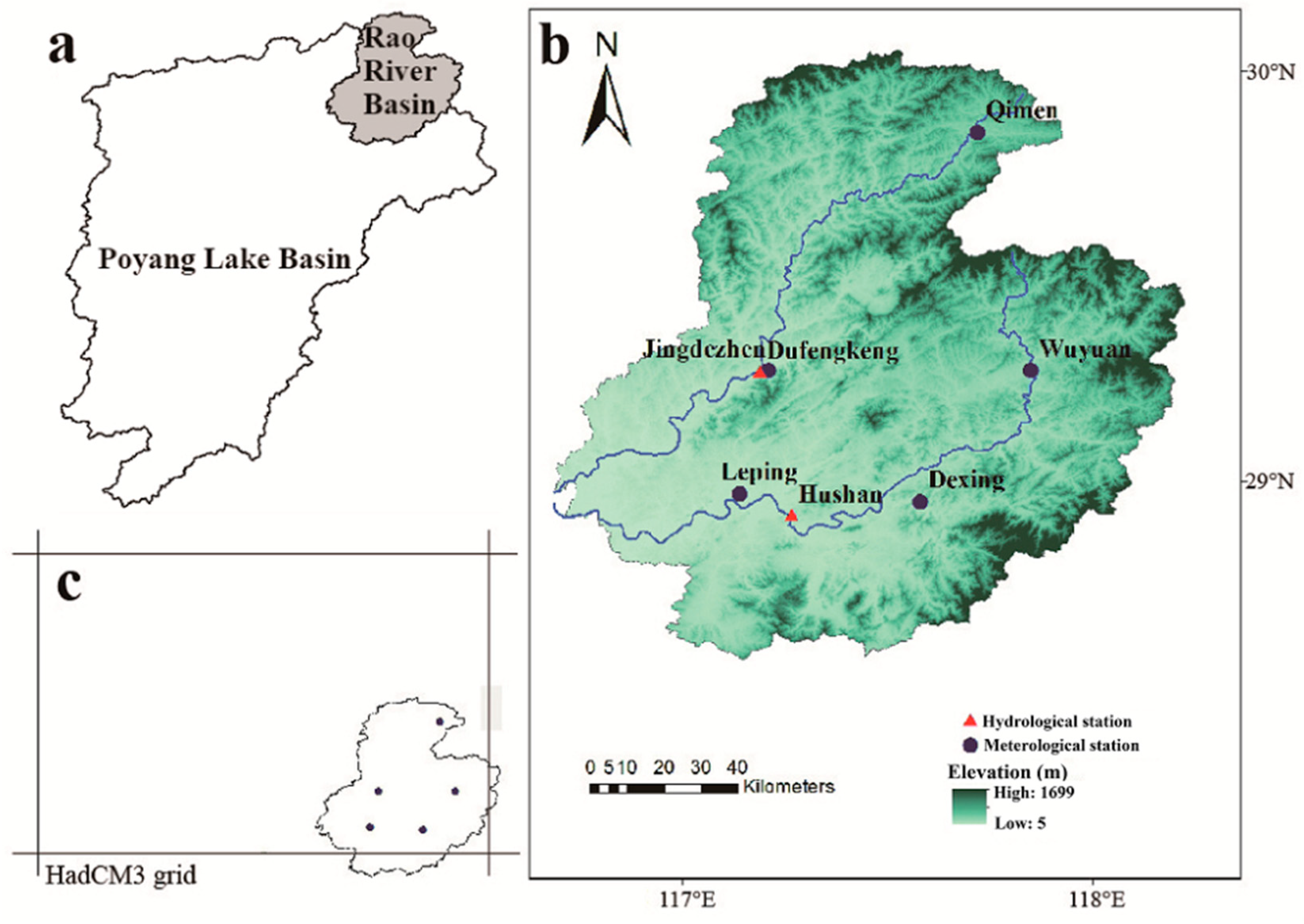
2.1. Study Area and Data

The Rao River, which is one of the five major rivers of the Poyang Lake system, is located in the northeast section of the Poyang Lake basin (Figure 1a). The river has two tributaries known as the north branch (the Chang River, 5851 km²) and the south branch (the Le’an River, 8367 km²). Rainfall is unevenly distributed throughout the year. The precipitation from April to June accounts for more than 60% of the total annual rainfall. Floods occur mainly in this period of the year.

The data used in this study consists of (1) daily precipitation and daily mean temperature of five meteorological stations in the study area from 1961 to 2000, and (2) daily mean streamflow of two hydrological stations from 1961 to 2000. The distribution of meteorological and hydrological stations is shown in Figure 1b, (3) NCEP reanalysis data, (4) daily data for atmospheric variables in the A2 and B2 scenarios of the global climate model HadCM3 of the Hadley Center for Climate Prediction and Research [37]. The spatial resolution of NCEP (1961–2000 period) is the same as that of the HadCM3 model (1961–2099 period), which is 3.75° (longitude) × 2.5° (latitude). Both NCEP reanalysis data and HadCM3 data are predictors in the SDSM model, and have been normalized with respect to their 1961–1990 means and standard deviations. Because the former can better reflect the actual climate state, it is used to establish the statistical relationship with the predictions (precipitation or temperature). HadCM3 data are taken into the established statistical relationship to generate downscaled precipitation/temperature. The corresponding HadCM3 grid points of the meteorological and hydrological stations are shown in Figure 1c.

In this study, the flood and drought are defined based on daily mean streamflow data. The flood refers to the annual maxima of the daily mean streamflow series, and the drought refers to the annual minima of the daily mean streamflow series. The common definition of drought is a sequence of low precipitation or streamflow values and should be characterized by its length (or duration), intensity, and severity. However, this research assumed a simplification. The definition of drought in this research is based on the encounter probability model, and the encounter probability of occurrence dates is defined based on the dates in which the drought (or flood) occurs. Therefore, we use the annual minima of the daily mean streamflow to define drought.

2.2. SDSM Method

Statistical downscaling is used to obtain small-scale information by establishing a statistical relationship between predictands and predictors.

$$Y=F\left(X\right),$$

(1)

where Y represents a small-scale predictand, X represents large-scale climate predictors, and F represents the statistical relationship between Y and X.

SDSM achieves the predictor-predictand conversion by combining multi-variate regression with the stochastic weather generator [13,18]. As a parameter of the local weather generator, the large-scale predictor is used to determine whether precipitation occurs and to provide the random variation of precipitation during wet days. This method can be expressed by the equation below.

$${\omega }_t={\alpha }_0+{\sum }_{j-1}^n{\alpha }_j{\widehat{u}}_i^{\left(j\right)}+{\alpha }_{t-1}{\omega }_{t-1},$$

(2)

where ${\omega }_t$ is the conditional probability of precipitation on day t, ${\widehat{u}}_i^{\left(j\right)}$ is the standardized jth predictor, ${\alpha }_j$ is the regression coefficient calculated by the least-squares method, and ${\omega }_{t-1}$ and ${\alpha }_{t-1}$ are the probability of precipitation and the corresponding regression coefficient on day t−1. The values of these two parameters depend on the characteristics of the study area and the predictand. A uniformly distributed random number $r_t$ (0 ≤ $r_t$ ≤ 1) is generated to determine a wet day when ${\omega }_t$ ≤ $r_t$ and a dry day when $r_t$ < ${\omega }_t$.

On wet days, the normalized precipitation Z can be represented by the equation below.

$$Z_t={\beta }_0+{\sum }_{j=1}^n{\beta }_j{\widehat{u}}_i^{\left(j\right)}+{\beta }_{t-1}{Z}_{t-1}+\epsilon ,$$

(3)

where $Z_t$ is the value of Z on day t, ${\beta }_j$ is the estimated regression parameter, ${\beta }_{t-1}$ and $Z_{t-1}$ are the regression parameter and Z on day t−1, and $\mathsf{\epsilon }$ is the stochastic component of the normal distribution.

With the $Z_t$, the precipitation $y_t$ on day t can be expressed by the equation below.

$$y_t=F{}^{-1}\left[\varnothing \left(Z_t\right)\right],$$

(4)

where $\varnothing$ is the normal cumulative distribution function, and $F$ is the empirical distribution function of $y_t$.

For temperature, there is only randomness on how high the temperature fluctuates, which can be represented similarly to Equations (3) and (4). After calibration, one can evaluate the downscaling model with statistics such as the coefficient of determination (R²) and root mean square error (RMSE).

2.3. The Xin’anjiang Model

The Xin’anjiang model is a watershed hydrological model that is widely used for hydrological simulation and prediction in humid and sub-humid regions [38]. The three-water-source Xin’anjiang model used in this paper includes the calculations of evapotranspiration, runoff yield, water source separation, and runoff concentration. The inputs are precipitation (P) and potential evapotranspiration (PET), while the output is the streamflow (Q) at the basin’s outlet.

To assess the goodness-of-fit between the simulated and observed streamflow, according to the Standard for Hydrological Information and Hydrological Forecasting (SHIHF) [39], Nash-Sutcliffe efficiency (NSE) is used to measure the accuracy.

$$\mathrm{NSE}=1-\frac{{\sum }_{i=1}^n{[y_c\left(i\right)-y_0\left(i\right)]}^2}{{\sum }_{i=1}^n{[y_0\left(i\right)-{\overline{y}}_0]}^2},$$

(5)

where NSE is the Nash-Sutcliffe efficiency, $y_c\left(i\right)$ is the simulating value, $y_0\left(i\right)$ is the observed value, ${\overline{y}}_0$ is the mean of the observed value, and n is the length of the data series. The forecast accuracy is classified into Grade A, B, and C, when NSE ≥ 0.90, 0.90 > NSE ≥ 0.70, and 0.70 > NSE ≥ 0.50, respectively. Only when the accuracy of prediction reaches grade A or B, can it be accepted for further analysis.

PET represents the maximum evapotranspiration that can occur from a given underlying surface under certain meteorological conditions when the water supply is not limited [40]. The Hamon method is one of the common methods to calculate PET, which is simple in calculation and superior in performance [40,41,42]. We chose the Hamon method to calculate PET because we do not have the radiation data, which is a requirement in most of the other methods. The calculated PET is used as input for further analysis of the Xin’anjiang model.

2.4. Encounter Probability Model

(1) Marginal Distribution

Flood occurrence dates are first converted to the radian t ($t=D_j\times 2\pi /L$, where $D_j$ represents the observed flood of the jth year that occurs on the day $D_j$ of the flood season of the length $L$). Since the probability density function of the flood occurrence dates can be either unimodal or multimodal, the mixed von Mises distribution (i.e., the probability density function of the flood occurrence dates t) is selected as follows.

$$\mathrm{f}\left(t\right)={\sum }_{i=1}^m\frac{p_i}{2\pi I_0\left({\kappa }_i\right)}\exp \left[{\kappa }_i\cos \left(t-{\mu }_i\right)\right],0\le t\le 2\pi ,0\le {\mu }_i\le 2\pi ,{\kappa }_i>0,$$

(6)

where i is the component of the mixed von Mises distribution, m is the number of components, $p_i$ is the mixing ratio, ${\mu }_i$ is the location parameter, ${\kappa }_i$ is the scale parameter, and $I_0\left({\kappa }_i\right)$ is the first-class Bessel function with a zero-order correction.

According to the Regulations for Calculating Design Flood of Water Resources and Hydropower Projects [43], the Pearson type III (P-III) distribution is used as the marginal distribution of the flood magnitudes q, and its probability density function is shown below.

$$\mathrm{f}\left(q\right)=\frac{{\beta }^{\alpha }}{\Gamma \left(\alpha \right)}{(q-\delta )}^{\alpha -1}\exp \left[-\beta \left(q-\delta \right)\right],\alpha >0,\beta >0,\delta \le q<\infty ,$$

(7)

where $\alpha$,$\beta ,$ and $\delta$ are the shape, scale, and location parameters of the P-III distribution, and $\Gamma \left(\alpha \right)$ is the gamma function.

Similarly, this method can be applied to the marginal distribution of the occurrence dates and magnitudes of drought.

(2) Joint Distribution

The copula function is a multivariate joint distribution function that is uniformly distributed from zero to one. Assuming that $F_{X_1}\left(x_1\right)$ and $F_{X_2}\left(x_2\right)$ are the marginal distribution functions of the random variables $X_1$ and $X_2$, the joint distribution function of $X_1$ and $X_2$ defined by the two-variable copula function is shown below.

$$F\left(x_1,x_2\right)=C\left(F_{X_1}\left(x_1\right),F_{X_2}\left(x_2\right)\right)=C\left(u,v\right),$$

(8)

where the copula function C connects the marginal distribution of two random variables, forming the joint distribution of the two variables.

The Archimedean copula function is frequently used due to its simple structure, ease of calculation, variety of forms, and great adaptability [44,45].

Table 1. Several types of the two-dimensional Archimedean Copula function.

Types	Copula Formula	The Relationship between θ and τ
Gumbel-Hougaard (GH)	$C(u,v)=\exp \{-{[{(-\ln u)}^{\theta }+{(-\ln v)}^{\theta }]}^{1/\theta }\}$	$\tau =1-\frac{1}{\theta },\theta \in [1,\infty )$
Clayton	$C(u,v)={(u^{-\theta }+v^{-\theta }-1)}^{-1/\theta }$	$\tau =\frac{\theta }{\theta +2},\theta \in (0,\infty )$
Frank	$C(u,v)=-\frac{1}{\theta }\ln [1+\frac{(e^{-\theta u}-1)(e^{-\theta v}-1)}{e^{-\theta }-1}]$	$\tau =1+\frac{4}{\theta }[\frac{1}{\theta }{\displaystyle {\int }_0^{\theta }\frac{t}{\exp (t)-1}}dt-1],\theta \in R$

shows several common two-dimensional Archimedean copula functions. The relationship between the parameter (θ) of the copula function and the Kendall rank correlation coefficient (τ) is used to estimate θ.

The ordinary least square criterion (OLS) and Akaike information criterion (AIC) are used to evaluate the fitting of the copula function [46]. The smaller the OLS value (AIC value) is, the better the fit of the copula function will be.

(3) Establishment of the Encounter Probability Model

The copula function is used to represent the joint distributions of the flood occurrence date and flood magnitudes at the two hydrological control stations of the tributaries of the Rao River.

$$\mathrm{F}\left(t_D,t_H\right)=C\left(F_{T_D}\left(t_D\right),F_{T_H}\left(t_H\right)\right),$$

(9)

$$\mathrm{F}\left(q_D,q_H\right)=C\left(F_{Q_D}\left(q_D\right),F_{Q_H}\left(q_H\right)\right),$$

(10)

where $T_D$ and $T_H$ represent the flood occurrence dates at Dufengkeng Station (D) in the Chang River and Hushan Station (H) in the Le’an River. $Q_D$ and $Q_H$ represent the flood magnitudes at the two stations. $F_{T_D}\left(t_D\right)$ and $F_{T_H}\left(t_H\right)$ are the marginal distributions of the flood occurrence dates at the two stations and $F_{Q_D}\left(q_D\right)$ and $F_{Q_H}\left(q_H\right)$ are the marginal distributions of the flood magnitudes at the two stations.

A flood encounter occurs when the flood of the two tributaries appear on the same day. When the flood magnitudes are not considered, the flood encounter refers to the dates when a flood encounter occurs. There are some limitations due to the simplification of our model design. This study does not take into account the situation that the floods occurred on adjacent dates in the two tributaries, which will also lead to a large flood downstream. The probability of the maximum flood occurrence date of the two tributaries on the ith day is shown below.

$$\begin{array}{c}{p}_i=P\left(t_i\le T_D<t_{i+1},t_i\le T_H<t_{i+1}\right)=F_T\left(t_i,t_i\right)+F_T\left(t_{i+1},t_{i+1}\right)-F_T\left(t_i,t_{i+1}\right)-\\ F_T\left(t_{i+1},t_i\right),\end{array}$$

(11)

where $F_T\left(t_i,t_j\right)$ is the joint probability of the maximum annual flood occurring before day i in station D and day j in station H.

The probability of flood occurrence in the flood season is shown below.

$$P_T=\sum p_i,$$

(12)

The probability of the two tributaries experiencing a flood greater than a particular magnitude (or within a particular return period) is shown below.

$$p^T=P\left(Q_D>q_D^T,Q_H>q_H^T\right)=1-F_{Q_D}\left(q_D\right)-F_{Q_H}\left(q_H\right)+F\left(q_D,q_H\right),$$

(13)

where $Q_D$ and $Q_H$ represent the flood magnitudes at stations D and H, and $q_D^T$ and $q_H^T$ are the design floods of the two tributaries with T-year return periods. Since the correlation between the dates and the magnitudes of the maximum flood occurrence is small, they can be regarded as independent events. In the flood season, the probability of the two tributaries experiencing flood occurrence and both of the floods greater than a certain magnitude (a particular return period) is shown below.

$$P=P_T\times P^T,$$

(14)

The establishment of the encounter probability model of drought is the same as that of flood. However, the probability in Equation (13) needs to be changed to that of the two tributaries experiencing a drought smaller than a particular magnitude (or within a particular return period), which is shown below.

$$p^T=P\left(Q_D<q_D^T,Q_H<q_H^T\right)=\mathrm{F}\left(q_D,q_H\right),$$

(15)

3. Results and Discussion

3.1. Predictions of Future Precipitation and Temperature

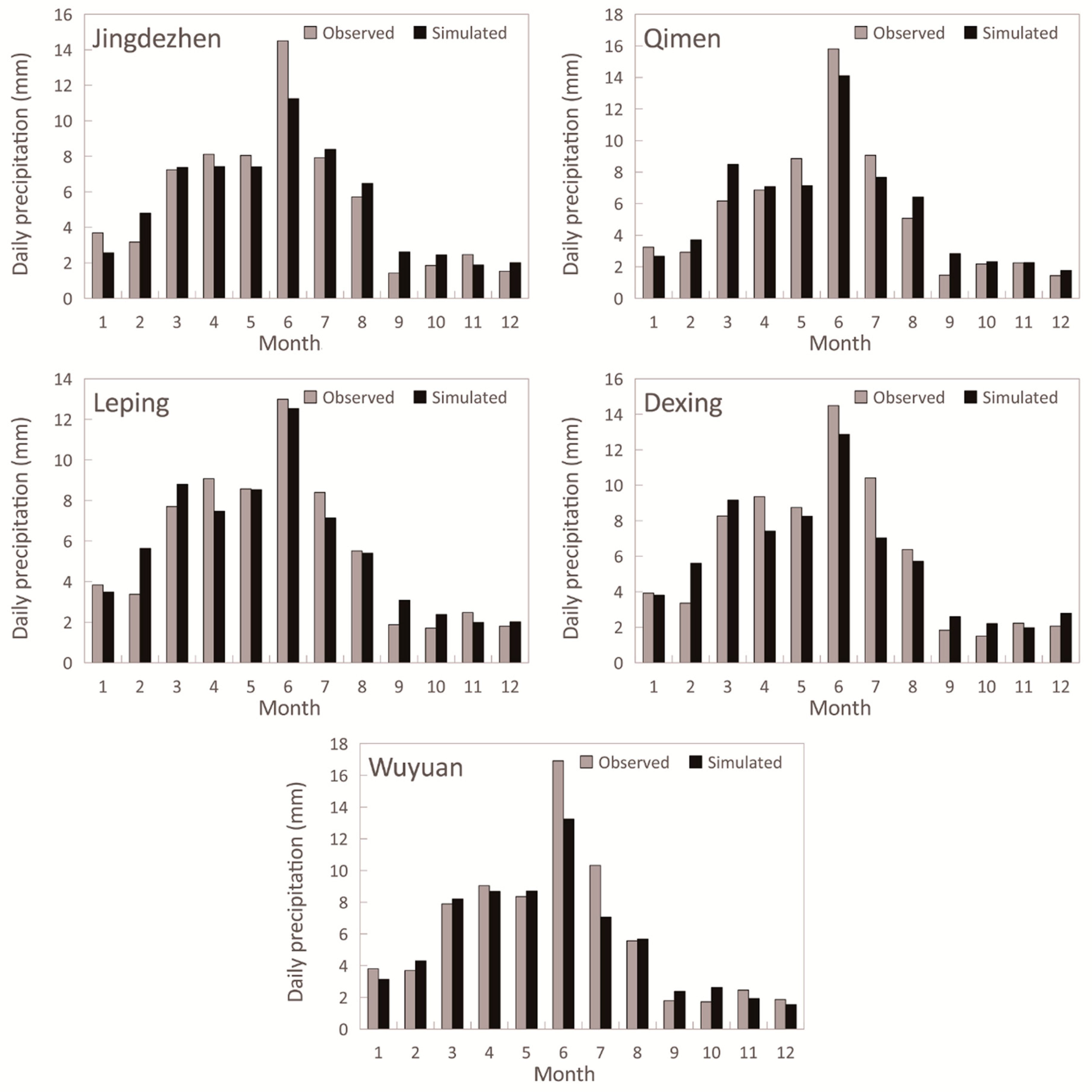
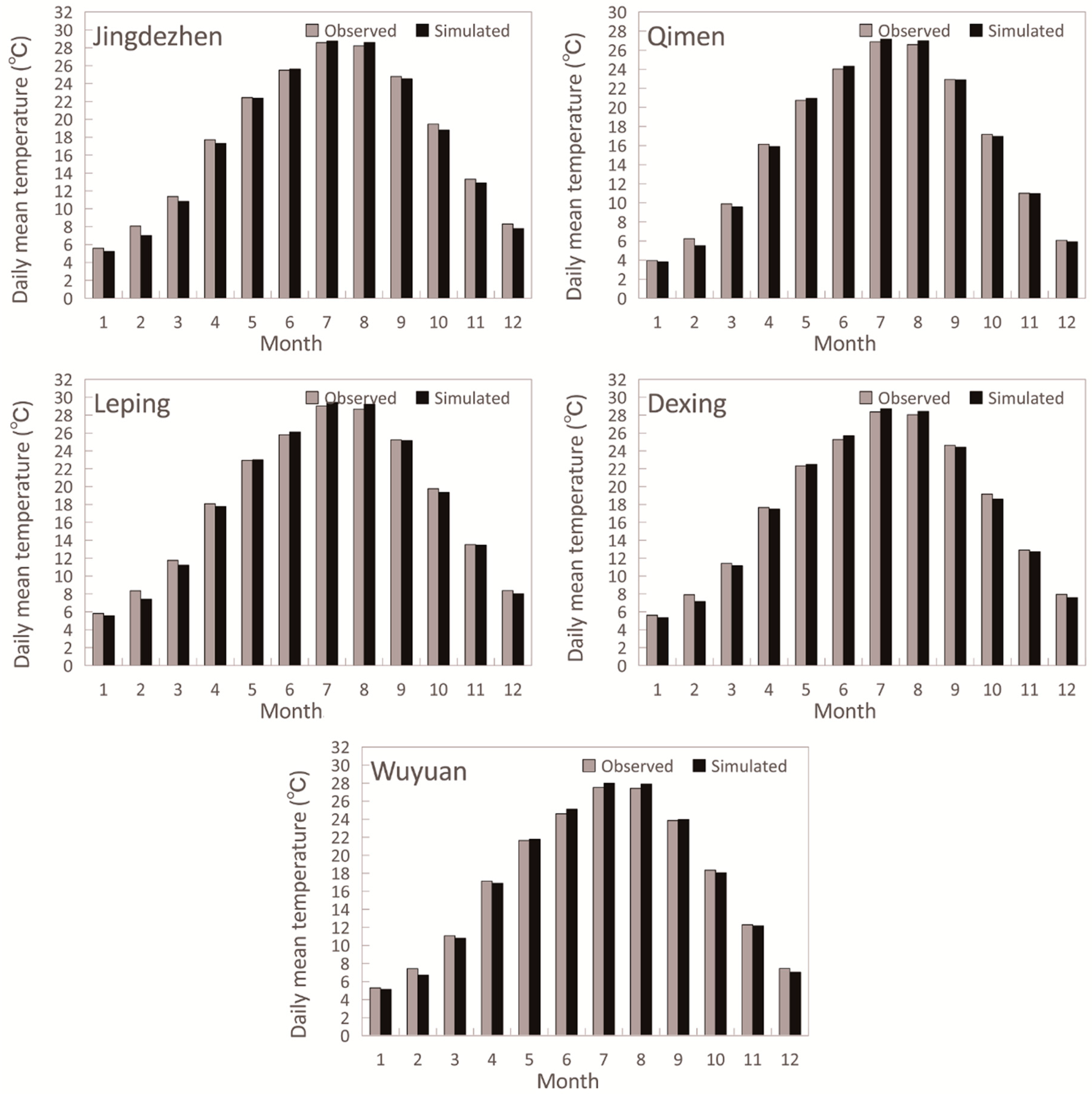
3.1.1. Calibration and Validation of SDSM

SDSM was used to establish a statistical model between large-scale predictors and regional predictands. The predictors suitable for downscaling of daily precipitation and daily mean temperature at five meteorological stations were selected from the 26 atmospheric predictor variables of the NCEP data. Predictors were screened based on the correlation between predictands and predictors. The explained variance and partial correlation coefficients between the two were used as screening criteria. The larger explained variance and partial correlation coefficient suggest a potentially reliable predictor. The predictors for the five stations in this study were screened station by station, and the selected predictors of each station are shown in

Table 2. Selected predictors for different predictands of the five meteorological stations in SDSM.

Predictands	Predictors
	Qimen	Jingdezhen	Leping	Dexing	Wuyuan
Precipitation (mm)	p5_v, p500, p8_z, r850, rhum	p5_v, p5th, p8_z, r500, r850, rhum	p5_v, p8_v, p8_z, r500, r850, rhum	p5_v, p500, p5th, p8_z, r500, r850, rhum	p5_v, p5th, p8_z, r500, r850, rhum
Temperature (℃)	mslp, p500, p850, shum, temp	mslp, p500, p850, shum, temp	mslp, p500, p850, shum, temp	mslp, p500, p850, shum, temp	mslp, p500, p850, shum, temp

Note: p5 and p8 represent 500 hPa and 850 hPa. v represents the meridional wind velocity. z represents the vorticity. th represents the wind direction. p500 and p850 represent the geopotential height of 500 hPa and 850 hPa. r500, r850, and rhum represent the relative humidity at 500 hPa, 850 hPa, and the sea level. mslp represents the mean sea level pressure. shum represents the specific humidity near the surface. temp represents the mean temperature.

.

Observed daily precipitation and daily mean temperature at the five meteorological stations and the selected predictors (in the period of 1961–2000) were used to calibrate and validate SDSM. Model calibration and validation were performed with data from 1961 to 1990 and from 1991 to 2000, respectively.

Table 3. The coefficient of determination (R²) and root mean square error (RMSE) of daily precipitation and daily mean temperature for each station in the calibration and validation periods.

Stations	Period	Precipitation (mm)		Temperature (°C)
		R2 (%)	RMSE (mm)	R2 (%)	RMSE (°C)
Jingdezhen	calibration	24.8	10.84	70.1	1.78
	validation	28.1	12.64	73.7	1.76
Qimen	calibration	38.1	11.1	71.8	1.66
	validation	29	14.1	73.4	0.63
Leping	calibration	26	11.21	70.9	1.78
	validation	31	13.61	72.6	1.78
Dexing	calibration	25.5	11.29	69.6	1.82
	validation	35.8	13.62	68.2	1.85
Wuyuan	calibration	26.7	11.23	69.1	1.78
	validation	34.1	14.23	69.8	1.77

shows the coefficient of determination (R²) and root mean square error (RMSE) of daily precipitation and daily mean temperature for each station in the model calibration and validation periods. The table demonstrates that, in the calibration period, R² for daily precipitation of the five meteorological stations was between 24.8% and 38.1%. RMSE was between 10.84 mm and 11.29 mm. R² for the daily mean temperature was between 69.1% and 71.8%, and RMSE was between 1.66 °C and 1.82 °C. In the validation period, R² for daily precipitation of the five meteorological stations was between 28.1% and 35.8%, and RMSE was between 12.64 mm and 14.23 mm. R² for the daily mean temperature was between 68.2% and 73.7%, and RMSE was between 0.63 °C and 1.85 °C. Precipitation downscaling is more problematic than temperature because daily precipitation amounts at individual sites are relatively poorly resolved by regional-scale predictors, and because precipitation is a conditional process in SDSM (i.e., both the occurrence and amount processes must be specified) [18]. Scholars used the SDSM model to downscale precipitation in different regions of the world. The average value of the coefficient of determination of daily precipitation is usually less than 30% [21,47,48]. Therefore, the coefficient of determination of precipitation in this paper indicates good performance of precipitation downscaling. Figure 2 and Figure 3 further demonstrate the observed and simulated daily precipitation and daily mean temperature for each month. Figure 2 illustrates that the SDSM model gave good simulation results for daily precipitation, and the simulated values in each month were similar to the observed values except for a few cases. Figure 3 shows that the simulated daily mean temperature over the whole year was close to the observed value. The fitting for each station in each month was satisfactory.

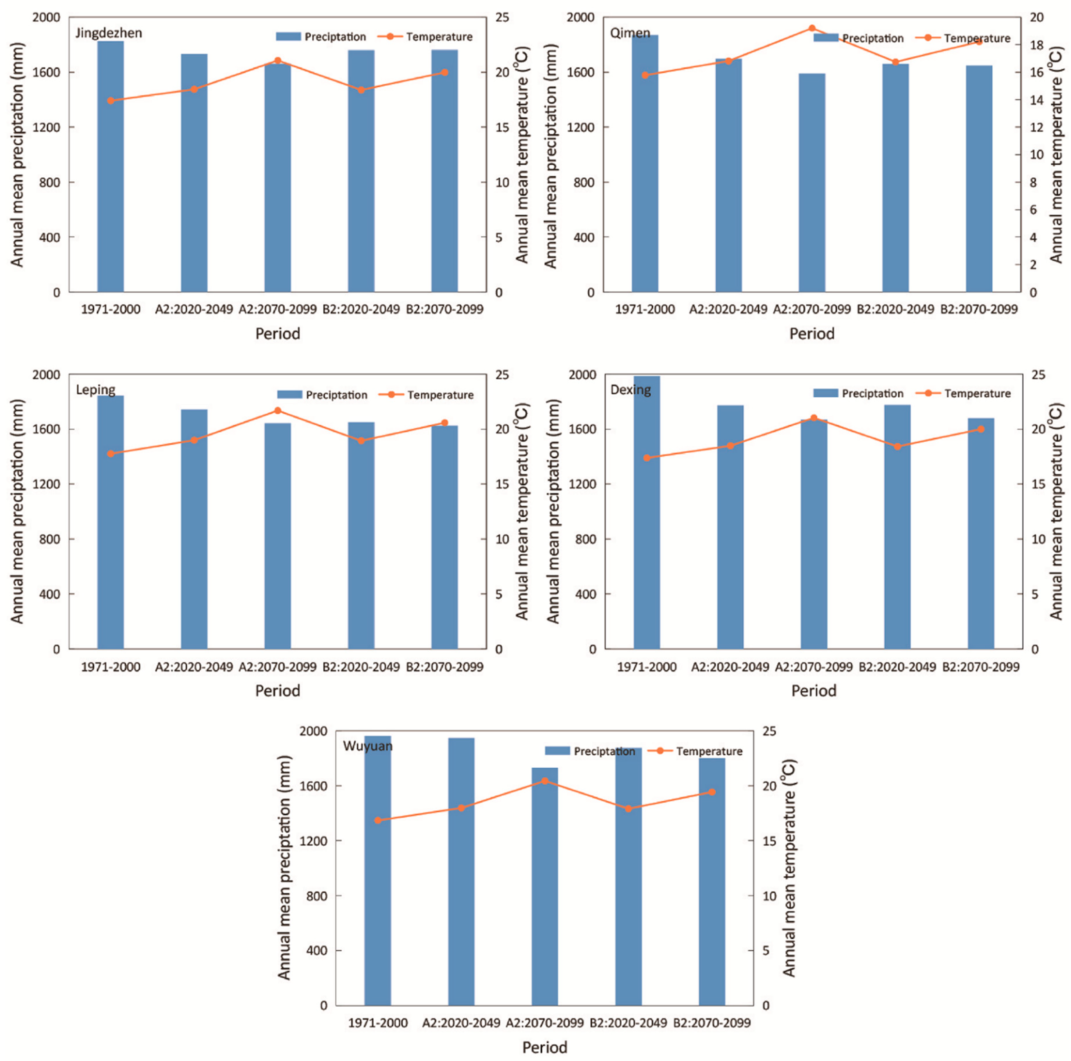
3.1.2. Predictions of Future Precipitation and Temperature

Based on the output of the HadCM3 model, the future daily precipitation and daily mean temperature for the five stations are predicted. Figure 4 represents annual mean precipitation and annual mean temperature for the two future periods under the A2 and B2 scenarios. The figure indicates that the annual mean precipitation decreases, while the annual mean temperature increases for the two future periods in both the A2 and B2 scenarios when compared with the reference period. These results are consistent with other independent studies using the most recent climate model outputs. For example, the projection by Guan [49] under the Representative Concentration Pathway (RCP) 4.5 scenario showed that the annual mean precipitation would decrease and the annual mean temperature would increase from 2020 to 2099 in most areas of the middle and lower reaches of the Yangtze River, China. Bao et al. [50] showed that the annual mean precipitation would decrease when compared with 1976–2005 in Southern China during 2031–2050 under RCP 4.5 scenario. Tian et al. [51] showed that the annual mean temperature continued to increase from the 1970s to the end of the 21st century in China under the RCP2.6, RCP4.5, and RCP8.5 scenarios.

3.2. Predictions of Future Runoff

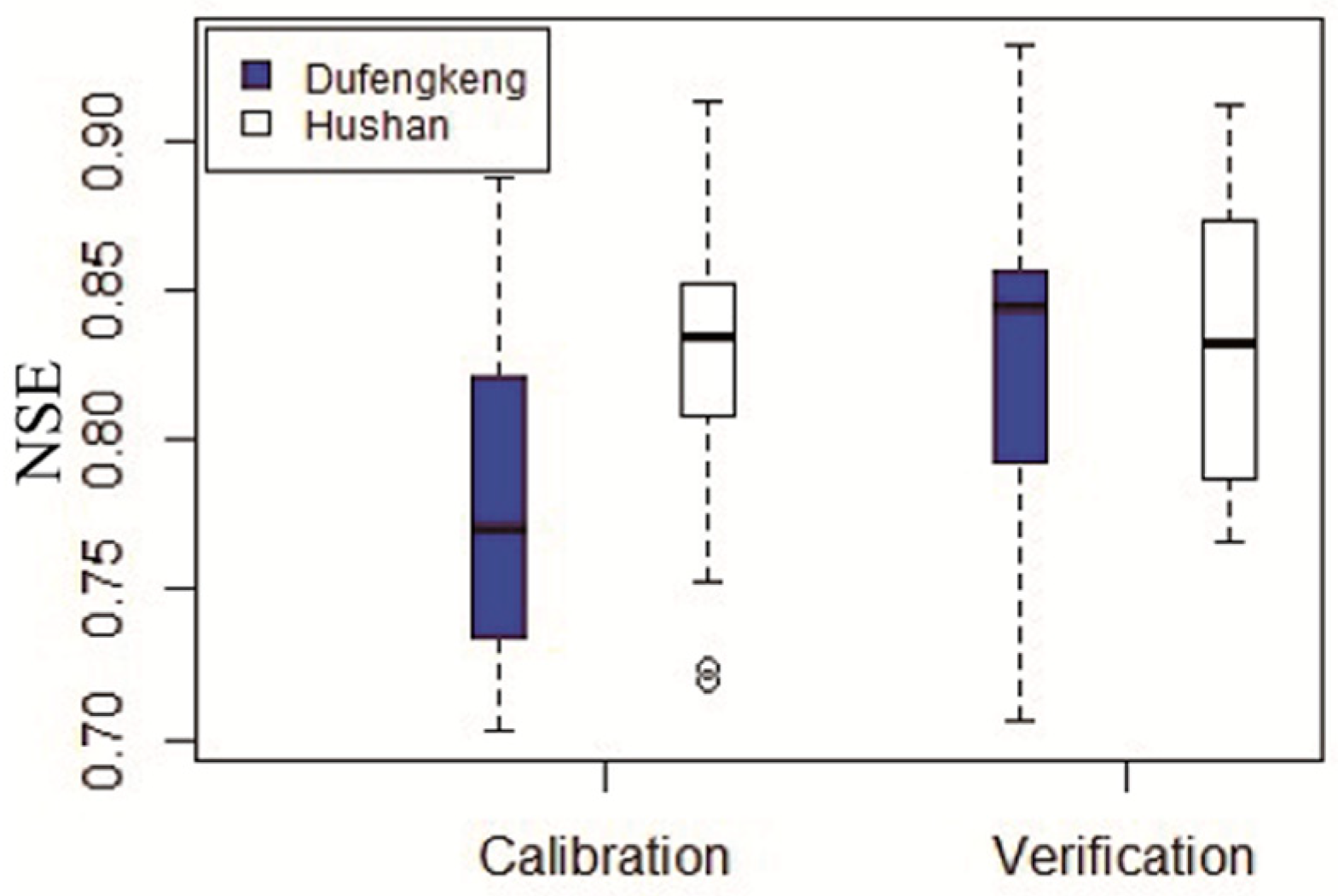
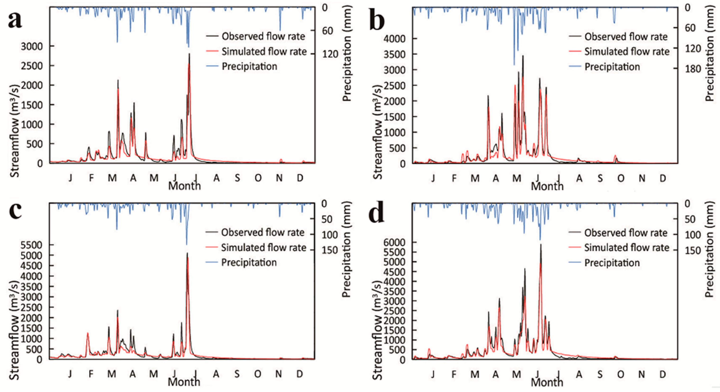
3.2.1. Calibration and Validation of the Xin’anjiang Model

Daily potential evapotranspiration was calculated by Hamon’s equation using the daily mean temperature. The daily precipitation and potential evapotranspiration were then used as inputs to the Xin’anjiang model to simulate the outlet daily mean streamflow of Dufengkeng Station and Hushan Station. The observed daily mean streamflow for the two stations in the period 1961–1990 and 1991–2000 were used for model calibration and validation, respectively. The calibrated parameters are shown in

Table 4. The calibrated parameters for the Xin’anjiang model.

Outlet Stations	WM	WUM	WLM	KE	B	SM	EX	CI	CG	IMP	C	KI	KG	N	NK
Dufengkeng	120	20	70	0.98	0.35	21	1.2	0.2	0.5	0.02	0.18	0.88	0.98	2	2.8
Hushan	120	20	70	0.85	0.40	25	1.2	0.2	0.5	0.02	0.18	0.90	0.98	2	2.8

Note: WM represents areal mean tension water capacity. WUM represents areal mean tension water capacity of the upper layer. WLM represents areal mean tension water capacity of the lower layer. KE represents the evaporation coefficient. B represents the tension water distribution index. SM represents the areal mean free water capacity of the surface soil layer. EX represents the free water distribution index. CI represents the recession constant of the interflow storage. CG represents the recession constant of the groundwater storage. IMP represents an impermeable coefficient. C represents a coefficient of deep evapotranspiration. KI represents outflow coefficients of the free water storage to interflow. KG represents outflow coefficients of the free water storage to groundwater. N represents the parameter n of the Nash model. NK represents the number of time steps.

.

Boxplots of the calculated Nash-Sutcliffe efficiency (NSE) of each year for the calibration and validation periods are shown in Figure 5. It shows that the medians of NSE for the Dufengkeng Station and Hushan Station were 0.771 and 0.835 in the calibration period and were 0.845 and 0.832 in the validation period. The range of NSE for Dufengkeng Station and Hushan Station were within 0.703–0.888 and 0.720–0.913 in the calibration period and were within 0.706–0.931 and 0.766–0.912 in the validation period. Therefore, all NSE of the two stations were >0.7, which met the precision requirements of SHIHF. Figure 6 compares the observed and simulated streamflow for Dufengkeng Station and Hushan Station in the calibration and validation periods (in the cases of 1966 and 1995 with moderate simulation results). The simulated streamflow is close to the observed one, which demonstrates the ability of the constructed Xin’anjiang model in simulating the streamflow process in the two hydrological stations.

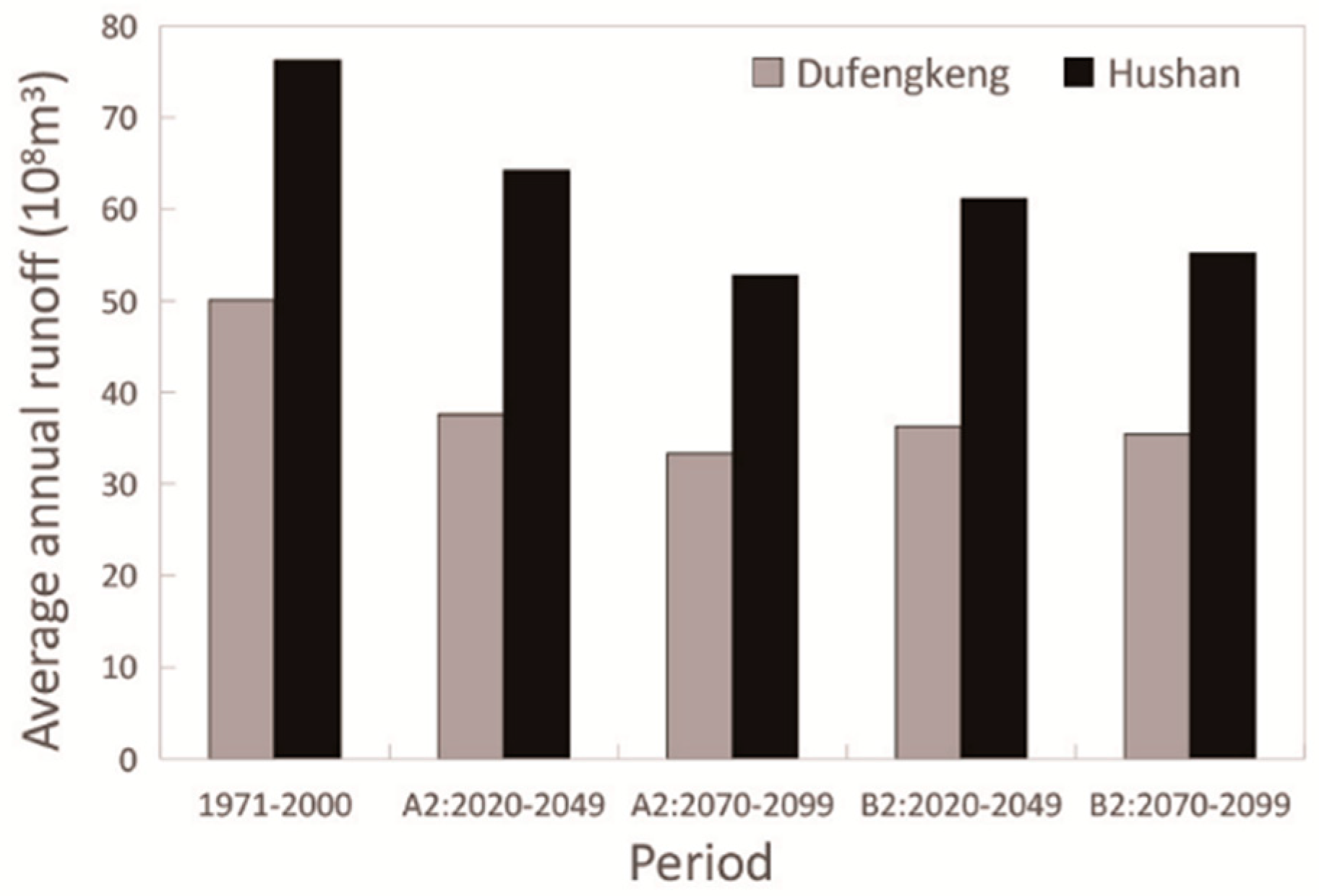
3.2.2. Predictions of Future Runoff

Predicted daily mean streamflow for Dufengkeng Station and Hushan Station in the periods of 2020–2049 and 2070–2099 were obtained from the calibrated Xin’anjiang model using predicted future daily precipitation and potential evapotranspiration. Figure 7 shows the average annual runoff for both stations for the two future periods in the A2 and B2 scenarios. As can be seen, the runoff would decrease for the two future periods in both the A2 and B2 scenarios when compared with the reference period. These results are consistent with the findings from Liu et al. [52], who also showed that the future annual runoff would decrease in the Rao River basin under A2 and B2 scenarios. The runoff of the same future period has few differences in these two scenarios, while the runoff in the second period is less than that of the first period, which shows the decrease of available water resources.

3.3. Probability Analysis of Future Flood Encounters

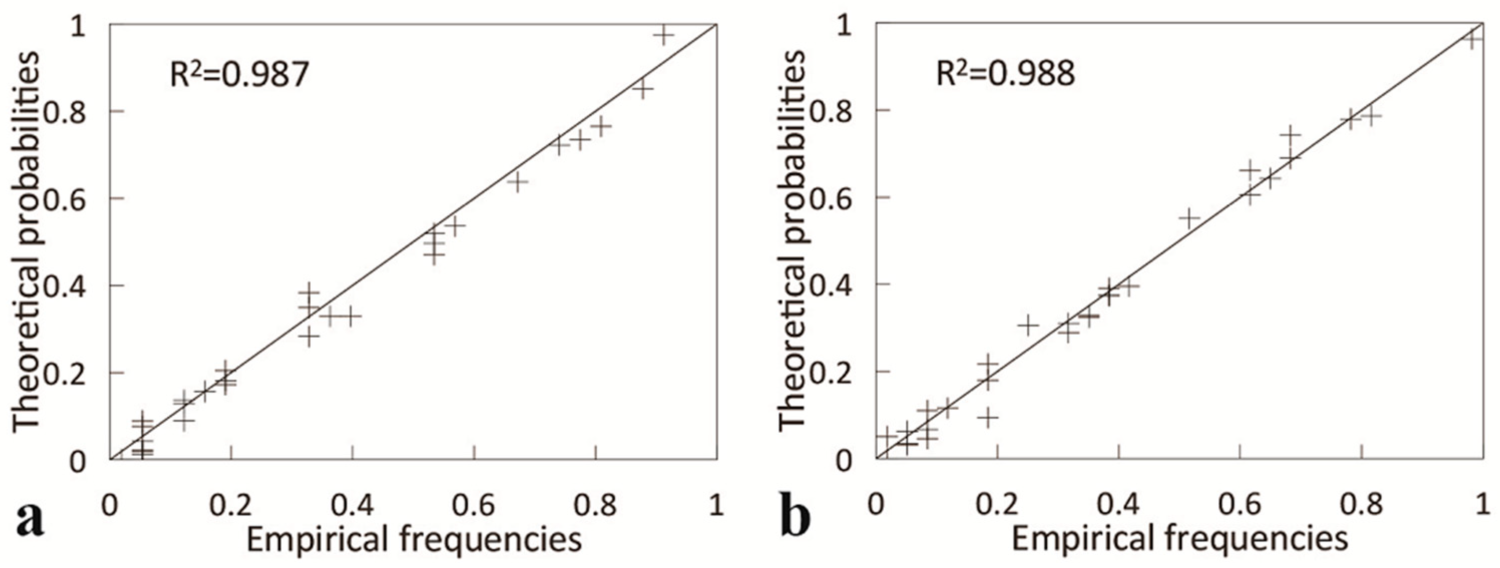
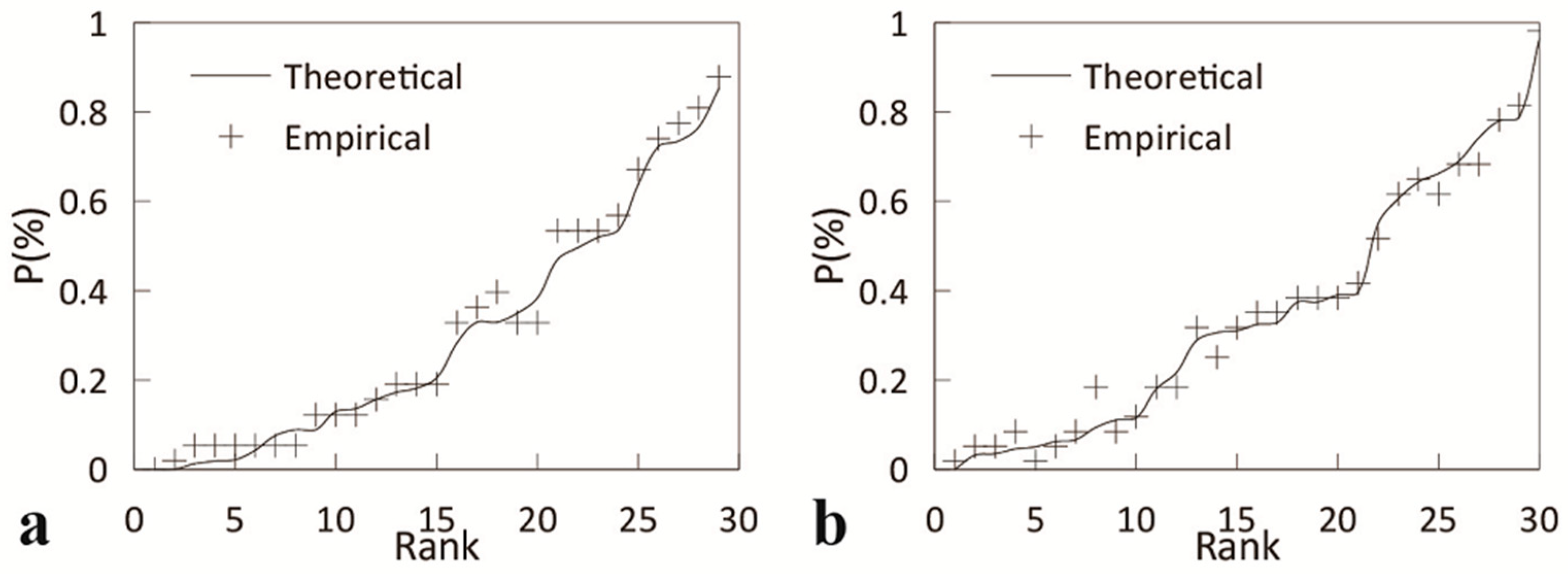
3.3.1. Establishment of the Marginal Distribution

The flood, mainly occurring in the flood season (April-September), refers to the annual maxima of the daily mean streamflow series in this study. The occurrence dates of the flood can be treated as a circular quantity and, thus, were converted into radians. The mixed von Mises distribution was used to fit the marginal distribution of flood occurrence dates, and the parameters were estimated by the maximum likelihood method. The Pearson type III (P-III) distribution was used to fit the marginal distribution of the flood magnitudes, and the parameters were estimated using L-moments.

Table 5. Marginal distribution parameters and RMSE between the theoretical probability and the empirical frequency for Dufengkeng Station and Hushan Station in the reference period.

Stations	Mixed von Mises Distribution				Pearson Type III Distribution
	Ρi	Κi	μi	RMSE	α	β	δ	RMSE
Dufengkeng	0.14	40.11	2.96	0.023	1.25	1478.44	1308.52	0.033
	0.19	1.12	1.57
	0.39	22.56	3.26
	0.28	3.92	2.36
Hushan	0.21	12.92	0.5	0.029	20.55	329.16	−2906.34	0.028
	0.21	52.16	2.96
	0.22	27.52	3.31
	0.36	3.15	2.61

shows the marginal distribution parameters and RMSE between the theoretical probability and the empirical frequency for Dufengkeng Station and Hushan Station in the reference period. The marginal distribution of the flood occurrence dates has 3 × 4 parameters since the probability density function is multimodal.

Table 6. Parameter estimation and fitting results for the joint distribution of flood occurrence dates and magnitudes in the reference period.

Types	Occurrence Dates			Magnitudes
	θ	OLS	AIC	θ	OLS	AIC
GH	1.54	0.035	−198.90	1.66	0.03	−207.55
Clayton	1.09	0.046	−182.31	1.32	0.046	−182.31
Frank	3.54	0.038	−194.28	4.12	0.038	−194.28

indicates that the RMSE values for the marginal distributions of the occurrence dates and magnitudes for the two stations are rather small, which justifies the selection of the mixed von Mises distribution and P-III.

The estimated flood quantiles in different return periods were calculated based on the marginal distribution of the flood magnitudes. The results show the return period of certain flood quantiles will be longer in the two future periods relative to the reference period for Hushan and Dufengkeng stations, which suggests a lower risk of a future major flood at each station. For instance, the estimated flood quantile of the 50-year-return-period at Hushan Station is 7262.88 m³/s, while the return period of such an estimated quantile in the future is about 60 years (A2: 2020–2049), 80 years (A2: 2070–2099), 180 years (B2: 2020–2049), and 300 years (B2: 2070–2099), respectively. The situation at Dufeng Station is the same as that of Hushan Station. These marginal distributions were then used to explore the flood encounter probability, which may significantly reinforce the severity of the flood disaster.

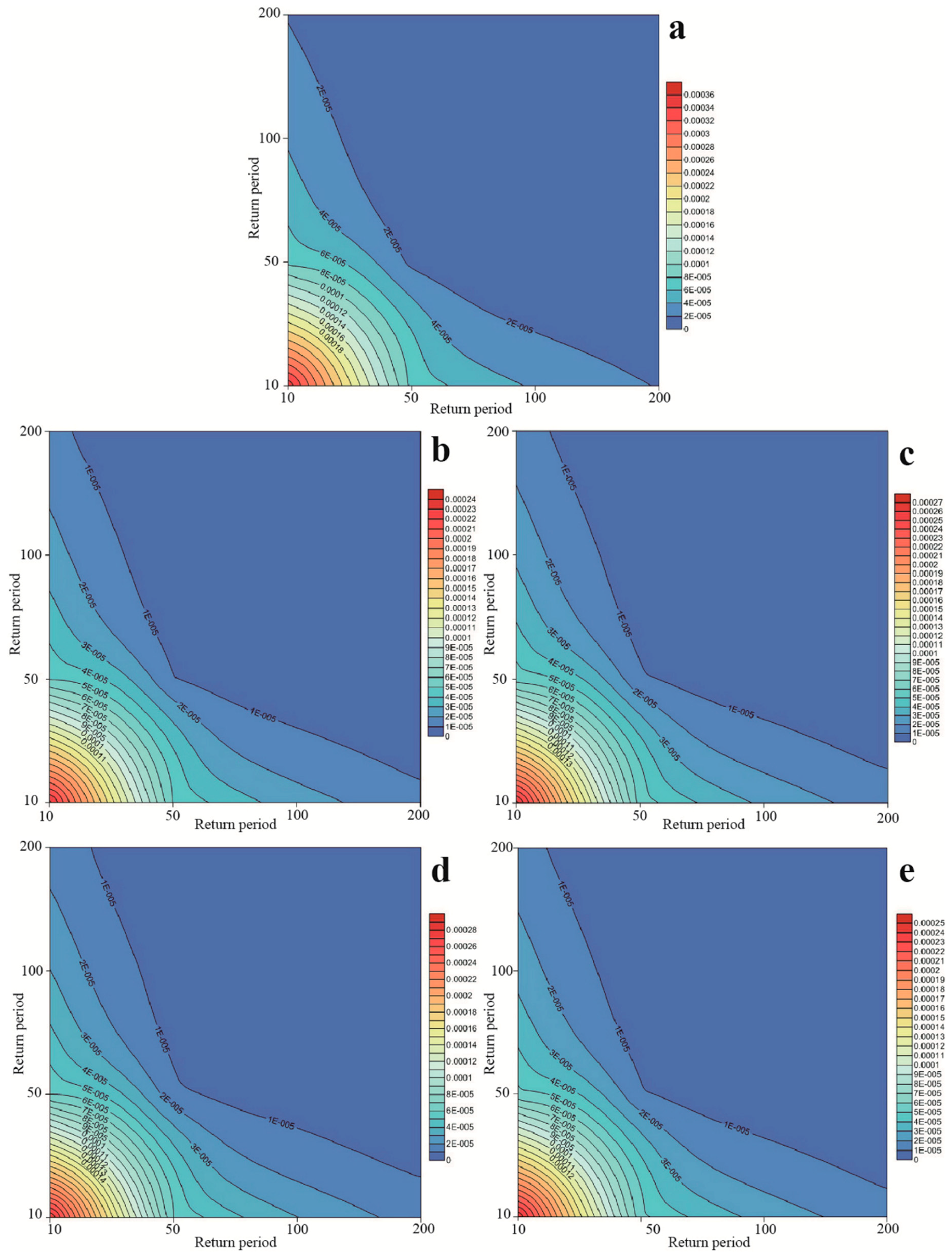
3.3.2. Establishment of the Joint Distribution

Kendall coefficients of rank correlation were used to calculate the parameters of three commonly used copula functions (see Table 1). The goodness of fit test was conducted on the three copula functions using the ordinary least square criterion (OLS) and the Akaike information criterion (AIC). Table 6 gives the parameters fitting results for the joint distribution of flood occurrence dates and magnitudes in the reference period. Table 6 implies that the Gumbel-Hougaard (GH) copula function has the least OLS and AIC values for both flood occurrence dates and magnitudes and, thus, was selected for the encounter probability study. Figure 8 shows the relevance between the empirical frequencies and theoretical probabilities of the flood occurrence dates and magnitudes when the GH copula function was used for the joint distribution, and Figure 9 shows the fitting results. Figure 8 indicates that the dots of empirical frequencies and theoretical probabilities fall near 1:1 line and that the coefficient of determination R² is larger than 0.98. The observed and the modeled distribution curves are close to each other (Figure 9), which justifies the application of the GH copula function for the joint distribution of flood occurrence dates and magnitudes.

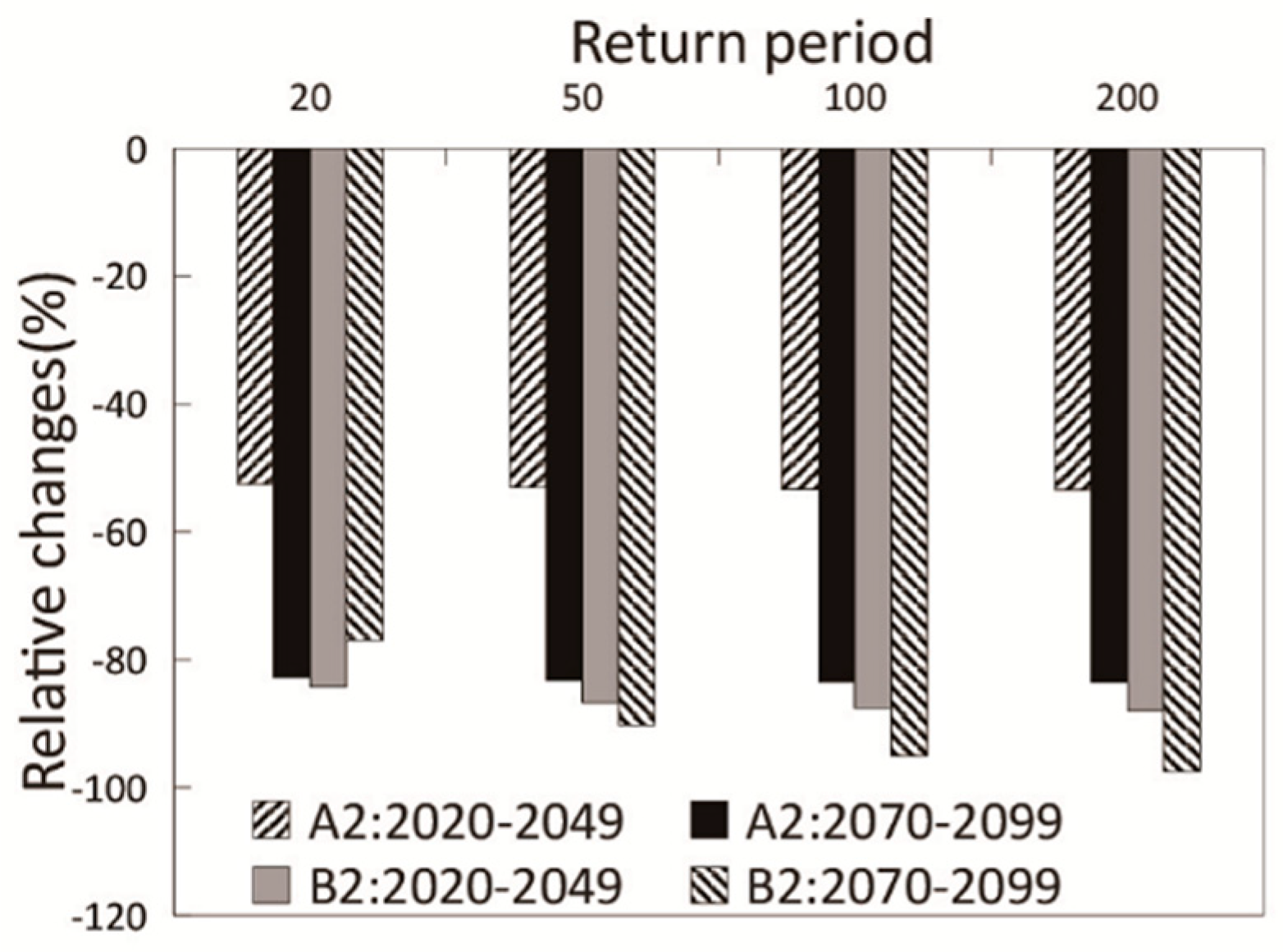
3.3.3. Flood Encounter Analysis

After the marginal distribution and joint distribution are obtained, the encounter probability model of flood occurrence dates and magnitudes can be established and analyzed. Figure 10 represents the encounter probability of flood occurrence dates in the flood season, derived from the two tributaries of the Rao River in the reference period and two future periods for the A2 and B2 scenarios. The flood encounter of the two tributaries might occur in late June to early July, with a probability >0.001 in the reference period. In the A2 and B2 scenarios, the flood encounter of the two tributaries is likely to occur from April to July in 2020–2049. In scenario A2, the flood encounter risk in late June and late July will be greater than that at other times, with the probabilities of about 0.00033 and 0.00037. In scenario B2, the flood encounter risk in early June and late June is greater than that at other times, with the probabilities of about 0.00047 and 0.00036. In both the A2 and B2 scenarios, floods of the two tributaries are both likely to occur in April and June in 2070–2099 and the encounter risk in April is greater than that in June, with the probabilities of about 0.00032 (scenario A) and 0.0018 (scenario B). Meanwhile, the cumulative encounter probability in the two future periods is smaller than that in the reference period. Generally, the flood encounter dates of the two tributaries in the reference period concentrate from late June to early July, and the encounter probability is relatively large. The flood encounter dates have multiple high probabilities in the flood season in the two future periods for the two scenarios, and the encounter probability is relatively small when compared with the reference period except for the period 2070–2099 in the B2 scenario. Furthermore, the flood encounter dates are generally earlier in the future scenarios than that in the reference period.

Figure 11 shows the flood encounter probability of the two tributaries of the Rao River for different return periods in the flood season during the reference period and the two future periods in the A2 and B2 scenarios. From this figure, one can obtain the flood encounter probability of the same-frequency flood and different-frequency flood in the two tributaries with different return periods (10, 50, 100, and 200 years, respectively). By analyzing the five subfigures, one can find that the flood encounter probability of the future two periods will decrease when compared with the reference period. For example, the encounter probability of floods with the same-frequency of 50-year-return-period in the reference period is about 0.00025, while the encounter probability of floods with different-frequency of a 50-year-return-period and a 100-year-return-period is about 0.00018. In the A2 scenario, the encounter probability of floods with the same-frequency of 50-year-return-period in the period of 2020–2049 is merely 0.00012, while the encounter probability of floods with different-frequency of 50-years and 100-years is 0.00008.

Figure 12 shows the changes in the encounter probability of the two tributaries in the two future periods of the A2 and B2 scenarios compared with the reference period. It can be seen from the figure that the encounter probability of floods with the same-frequency of 20-year, 50-year, 100-year, and 200-year in the period of 2020–2049 and 2070–2099 for both scenarios will decrease when compared with the reference period, which is reduced by more than 52% to 97%. That is, compared with the reference period, the encounter probability of floods with the same-frequency in the two future periods in both scenarios will decrease.

In summary, the probability of a future major flood at each station will decrease, according to the estimated quantiles of marginal distribution of flood, and the flood encounter probability of the two tributaries for different return periods will also decrease in the two future periods when compared with the reference period. This shows the reduced risk of future major flood in the study area.

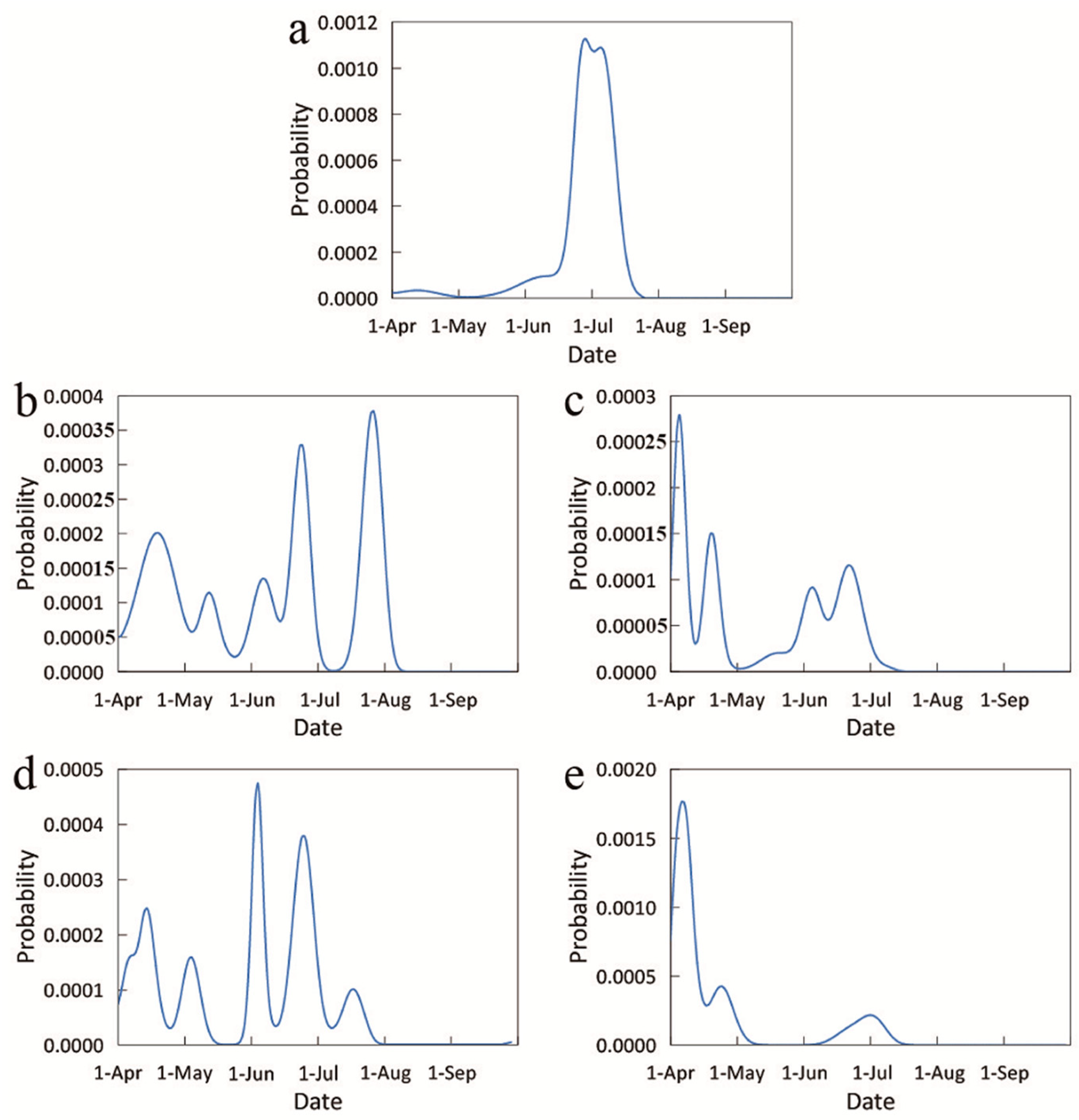
3.4. Probability Analysis of a Future Drought Encounter

The encounter probability of droughts was calculated in the same way as in Section 3.3. First, the annual minimum series of daily mean streamflow (refer to as drought in this study) for each station is selected. According to the analysis of the long-term series data in each station, the drought mainly occurred in the non-flood season (October-May). The mixed von Mises distribution and the P-III distribution are then used to establish the marginal distributions of the drought occurrence dates and magnitudes. Next, the marginal probability of future drought is also estimated in Section 3.3. Lastly, through the test, the GH Copula function is selected to calculate the joint distribution of the drought occurrence dates and magnitudes (the related figures and tables are not shown).

The estimated drought quantiles in different return periods were also calculated based on the marginal distribution of the drought magnitudes. Results show the return period of certain drought quantiles will be shorter in the two future periods relative to the reference period for Hushan Station and Dufengkeng Station, which suggests the increased probability of future major droughts at each station. For instance, the drought quantile of the 50-year-return-period at Hushan Station is 4.25 m³/s, while the return period of such an estimated quantile in the future is about 40 years (A2: 2020–2049), 10 years (A2: 2070–2099), 20 years (B2: 2020–2049), and 10 years (B2: 2070–2099), respectively. The situation at Dufeng Station is the same as that of Hushan Station.

Figure 13 presents the encounter probability of drought occurrence dates in the non-flood season, derived from the two tributaries in the reference period and two future periods for the A2 and B2 scenarios. First, different from the encounter probability of flood occurrence dates, which is generally unimodal in the reference period and two future periods (Figure 10), the encounter probability of the drought is primarily multimodal, that is, the encounter dates are more dispersed for the drought. Global warming not only can change the hydrometeorological process at an annual scale but also may alter the seasonality [53]. Monthly variations in precipitation and temperature may result in the multimodal encounter probability of drought (or flood) occurrence dates. It remains a challenging and open area of research that modeling climate change at high temporal resolutions [54,55]. Therefore, there are still some uncertainties. Next, although the encounter probability of drought occurrence dates in the two future periods is multimodal, the probability of the main peak is smaller than that in the reference period. The cumulative encounter probability in the two future periods is also smaller than that in the reference period. In terms of the encounter dates, the flood is advanced relative to the reference period under future climate scenarios, but the drought has no significant advance or delay. In summary, the drought encounter dates have multiple high probabilities in the non-flood season during the reference period and the two future periods in the two scenarios, and the encounter probability in the two future periods is relatively small when compared with the reference period.

Figure 14 shows the drought encounter probability of the two tributaries for different return periods in the non-flood season during the reference period and the two future periods in the A2 and B2 scenarios. From the figure, the encounter probability of the same-frequency drought and different-frequency drought in the two tributaries with different return periods (10, 50, 100, and 200 years, respectively) can be obtained. By analyzing the five subfigures, it can be seen that the drought encounter probability of the future two periods in the two scenarios will decrease compared with the reference period. For example, the encounter probability of drought with the same-frequency of a 50-year-return-period in the reference period is about 0.000016, while the encounter probability of drought with a different frequency of 50-year-return-period and 100-year-return-period is about 0.000008. In the A2 scenario, the encounter probability of drought with the same-frequency of a 50-year-return-period in the period of 2020–2049 is merely 0.000011. The encounter probability of drought with different-frequency of 50-years and 100-years is 0.000005.

Figure 15 represents the changes in the drought encounter probability of the two tributaries in the two future periods of the A2 and B2 scenarios compared with the reference period. The encounter probability of drought with the same frequency of 20-years, 50-years, 100-years, and 200-years in the period of 2020–2049 and 2070–2099 for both scenarios will decrease when compared with the reference period, which is reduced by 18% to 34%. That is, compared with the reference period, the encounter probability of drought with the same frequency in the two future periods in both scenarios will decrease, which is the same as the above conclusions.

The analysis of the major drought risk should consider comprehensively the changes of the single station probability and the encounter probability of the upstream stations. On the one hand, the probability of future major drought at each station will increase according to the estimated quantiles of the marginal distribution of drought. On the other hand, the drought encounter probability of the two tributaries for different return periods will decrease in the two future periods compared with the reference period. In summary, the risk of future major drought can be greater or lower compared with the reference period.

In this study, the risk of future major flood will mitigate, and the risk of future major drought can be greater or lower in the study area in the two future periods of the A2 and B2 scenarios when compared with the reference period. Arnell et al. [56] made an assessment of the implications of climate change for global river flood risk based on 21 climate models in the the Coupled Model Intercomparison Project Phase 3 (CMIP3) multi-model dataset. The results of some climate models indicated that the risk of flooding in East Asia would decrease in the future, which is consistent with the findings in this study. Sheffield et al. [57] predicted the changes of drought under future global warming from multiple models and scenarios. The results showed that the frequency of short-term droughts would increase from the mid-twentieth century to the end of the twenty-first century globally. The results of Lehner et al. [58] showed that Southeastern Asia saw no significant change in drought risk under any future scenario. Hirabayashi et al. [59] provided the global distribution of the multi-model median return period from 1971–2000 for the 100-year-return-period flood discharge in 2071–2100 in RCP scenarios. However, the results showed that the frequency of flood occurrence would increase (the return period decreases) across large areas of East Asia. The above literature shows that there are still many uncertainties in predicting future flood and drought risks in the context of climate warming.

The encounter probabilities and risk of floods and droughts will change under future climate change, according to our results. However, there are uncertainties in the prediction of future climate change based on GCMs. As for the significance of the changes, we are not sure about the magnitude of the changes, but are more concerned about the direction of the changes. Compared with the quantitative estimation of the changes of the encounter probabilities of future floods and droughts, this study pays more attention to understand whether the encounter probability and risk of flood and drought will change under future climate scenarios, so as to better cope with the future flood and drought disasters.

4. Conclusions

In this study, SDSM was used to generate future precipitation and temperature in the Rao River basin based on GCM data. Future streamflow in the Rao River basin was then obtained from the Xin’anjiang model utilizing the output from SDSM. The GH copula function was used to create an encounter probability model. The changes of future precipitation, temperature, and streamflow were studied and the changes in the encounter probabilities of flood and drought occurrences in the basin were further explored under the two climate scenarios of A2 and B2. The results of the research lead to the following conclusions.

(1) SDSM provided a good fit for future daily precipitation and daily mean temperature. The annual mean precipitation would decrease and the annual mean temperature would increase during the two future periods in the A2 and B2 scenarios when compared with the reference period. The Xin’anjiang model accurately simulated the daily mean streamflow at the hydrologic stations in the two tributaries of the Rao River. The average annual runoff would decrease in the two future periods for both scenarios.

(2) For flood occurrence dates, the encounter of the two tributaries’ floods concentrated from late June to early July in the reference period, while the encounter dates have multiple high probabilities in the flood season during the two future periods. The encounter probability of floods occurring in the flood season would both decrease in the two future periods, and the dates would generally be advanced under future climate change scenarios.

(3) For flood magnitudes, the encounter probability with the same frequency and different frequencies would both decrease in the two future periods when compared with the reference period (e.g., the encounter probability with the same-frequency of 100-year would reduce by 53% to 95%), and the probability of future flood at each station would also decrease. It indicates that the risk of a major flood would mitigate in the two future periods in the study area.

(4) For drought occurrence dates, the encounter dates of the two tributaries’ drought have multiple high probabilities in the non-flood season during the reference period and the two future periods in the two scenarios. The encounter probability would decrease in the two future periods when compared with the reference period.

(5) For drought magnitudes, the encounter probability with the same frequency and different frequencies would both decrease in the two future periods when compared with the reference period (e.g., the encounter probability with the same frequency of 100-years would reduce by 18% to 33%), but the probability of future drought at each station would increase. It indicates that the risk of future major drought can be greater or lower compared with the reference period.

This work is a new attempt on exploring the encounter probability and risk of future flood and drought of different sub basins under future climate change, using GCM data, a downscaling method, a hydrological model, and a copula function method. The results of this paper are helpful to understand the changes of flood and drought risk with the changes of occurrence time and magnitude of flood and drought under future climate scenarios.

We recognize that a single GCM may be limited for describing uncertainties in climate projections and new future climate scenarios of RCP can provide more updated information on climate change. However, the current study mainly focuses on the methodology to estimate the encounter probability and risk of future flood and drought. In addition, the methodology developed in this research will be easily applied in different regions in other climate models or scenarios.

References

1. Aalst, M.K.V. The impacts of climate change on the risk of natural disaster. Disasters 2006, 30, 5–18. [Google Scholar] [CrossRef]
2. Stott, P. How climate change affects extreme weather events. Science 2016, 352, 1517–1518. [Google Scholar] [CrossRef]
3. Toonen, W.H.J.; Middelkoop, H.; Konijnendijk, T.Y.M.; Macklin, M.G.; Cohen, K.M. The influence of hydroclimatic variability on flood frequency in the Lower Rhine. Earth Surf. Process. Landf. 2016, 41, 1266–1275. [Google Scholar] [CrossRef]
4. Forestieri, A.; Conti, F.L.; Blenkinsop, S.; Cannarozzo, M.; Fowler, H.J.; Noto, L.V. Regional frequency analysis of extreme rainfall in Sicily (Italy). Int. J. Climatol. 2018, 38, 698–716. [Google Scholar] [CrossRef]
5. Salvadori, G.; De Michele, C. Frequency analysis via copulas: Theoretical aspects and applications to hydrological events. Water Resour. Res. 2004, 40, 229–244. [Google Scholar] [CrossRef]
6. Chebana, F.; Ouarda, T.B.M.J. Multivariate quantiles in hydrological frequency analysis. Environmetrics 2011, 22, 63–78. [Google Scholar] [CrossRef] [Green Version]
7. IPCC. Climate Change 2014: Impacts Adaptation and Vulnerability and Climate Change 2014: Mitigation of Climate Change; Cambridge University Press: New York, NY, USA, 2014. [Google Scholar]
8. Wigley, T.M.L.; Jones, P.D.; Briffa, K.R.; Smith, G. Obtaining sub-grid-scale information from coarse-resolution general circulation model output. J. Geophys. Res. 1990, 95, 1943–1953. [Google Scholar] [CrossRef]
9. Robock, A.; Turco, R.P.; Harwell, M.A.; Ackerman, T.P.; Andressen, R.; Chang, H.S.; Sivakumar, M.V.K. Use of general circulation model output in the creation of climate change scenarios for impact analysis. Clim. Chang. 1993, 23, 293–335. [Google Scholar] [CrossRef]
10. Chen, J.; Brissette, F.P.; Leconte, R. Uncertainty of downscaling method in quantifying the impact of climate change on hydrology. J. Hydrol. 2011, 401, 190–202. [Google Scholar] [CrossRef]
11. Hellström, C.; Chen, D.L.; Achberger, C.; Räisänen, J. Comparison of climate change scenarios for sweden based on statistical and dynamical downscaling of monthly precipitation. Clim. Res. 2001, 19, 45–55. [Google Scholar] [CrossRef]
12. Murphy, J. An Evaluation of Statistical and Dynamical Techniques for Downscaling Local Climate. J. Clim. 1999, 12, 2256–2284. [Google Scholar] [CrossRef]
13. Wilby, R.L.; Dawson, C.W.; Barrow, E.M. SDSM—A decision support tool for the assessment of regional climate change impacts. Environ. Model. Softw. 2002, 17, 145–157. [Google Scholar] [CrossRef]
14. Shen, M.; Chen, J.; Zhuan, M.; Chen, H.; Xu, C.Y.; Xiong, L. Estimating uncertainty and its temporal variation related to global climate models in quantifying climate change impacts on hydrology. J. Hydrol. 2018, 556, 10–24. [Google Scholar] [CrossRef]
15. Corte-Real, J.; Quian, B.; Xu, H. Circulation patterns, daily precipitation in Portugal and implications for climate change simulated by the second Hadley centre GCM. Clim. Dyn. 1999, 15, 921–935. [Google Scholar] [CrossRef]
16. Mendez, F.J. Downscaling of global climate change estimates to regional scales: An application to Ierian rainfall. J. Clim. 1993, 6, 1161–1171. [Google Scholar] [CrossRef]
17. Wilks, D.S.; Wilby, R.L. The weather generation game: A review of stochastic weather models. Prog. Phys. Geogr. 1999, 23, 329–357. [Google Scholar] [CrossRef]
18. Wilby, R.L.; Dawson, C.W. Statistical Downscaling Model (SDSM), Version 4.2; Department of Geography, Lancaster University: Lancaster, UK, 2007. [Google Scholar]
19. Zhao, F.F.; Xu, Z.X. Statistical downscaling of future temperature change in source of the Yellow River Basin. Plateau Meteorol. 2008, 27, 153–161, (In Chinese with English abstract). [Google Scholar]
20. Souvignet, M.; Gaese, H.; Ribbe, L.; Kretschmer, N.; Oyarzun, R. Statistical downscaling of precipitation and temperature in north-central Chile: An assessment of possible climate change impacts in an arid Andean watershed. Hydrol. Sci. J. 2010, 55, 41–57. [Google Scholar] [CrossRef] [Green Version]
21. Gulacha, M.M.; Mulungu, D.M.M. Generation of climate change scenarios for precipitation and temperature at local scales using SDSM in Wami-Ruvu River Basin Tanzania. Phys. Chem. Earth 2017, 100, 62–72. [Google Scholar] [CrossRef]
22. Xiao, T.G. Analysis on flood encounter of Jinsha river and Minjiang river. Yangtze River 2001, 32, 30–32, (In Chinese with English abstract). [Google Scholar] [CrossRef]
23. Kim, G.; Silvapulle, M.J.; Silvapulle, P. Comparison of semiparametric and parametric methods for estimating copulas. Comput. Stat. Data Anal. 2007, 51, 2836–2850. [Google Scholar] [CrossRef]
24. Guo, S.L.; Yan, B.W.; Xiao, Y. Multivariate Hydrological Analysis and Estimation. J. China Hydrol. 2008, 28, 1–7, (In Chinese with English abstract). [Google Scholar]
25. Salvadori, G.; Michele, C.D.; Durante, F. Multivariate design via copulas. Hydrol. Earth Syst. Sci. Discuss. 2011, 8, 5523–5558. [Google Scholar] [CrossRef] [Green Version]
26. Michele, C.D.; Salvadori, G. A Generalized Pareto intensity-duration model of storm rainfall exploiting 2-Copulas. J. Geophys. Res. 2003, 108, 4067. [Google Scholar] [CrossRef]
27. Zhang, L.; Singh, V.P. Bivariate rainfall frequency distributions using archimedean copulas. J. Hydrol. 2007, 332, 109. [Google Scholar] [CrossRef]
28. Yan, B.W.; Guo, S.L.; Chen, L.; Liu, P. Flood encountering risk analysis for the Yangtze River and Qingjiang River. J. Hydraul. Eng. 2010, 39, 553–559, (In Chinese with English abstract). [Google Scholar] [CrossRef]
29. Bing, J.P.; Deng, P.X.; Zhang, X.; Lv, S.Y.; Marani, M.; Xiao, Y. Flood coincidence analysis of Poyang Lake and Yangtze River: risk and influencing factors. Stoch. Environ. Res. Risk Assess. 2018, 32, 879–891. [Google Scholar] [CrossRef]
30. Das, T.; Dettinger, M.D.; Cayan, D.R.; Hidalgo, H.G. Potential increase in floods in California’s Sierra Nevada under future climate projections. Clim. Chang. 2011, 109 (Suppl. 1), 71–94. [Google Scholar] [CrossRef]
31. Ryu, J.H.; Lee, J.H.; Jeong, S.; Park, S.K.; Han, K. The impacts of climate change on local hydrology and drought frequency in the Geum River Basin, Korea. Hydrol. Process. 2011, 25, 3437–3447. [Google Scholar] [CrossRef]
32. Tofiq, F.A.; Guven, A. Prediction of design flood discharge by statistical downscaling and General Circulation Models. J. Hydrol. 2014, 517, 1145–1153. [Google Scholar] [CrossRef]
33. Meaurio, M.; Zabaleta, A.; Boithias, L.; Epelde, A.M.; Sauvage, S.; Sánchez-Pérez, J.M.; Srinivasan, R.; Antiguedad, I. Assessing the hydrological response from an ensemble of CMIP5 climate projections in the transition zone of the Atlantic region (Bay of Biscay). J. Hydrol. 2017, 548, 46–62. [Google Scholar] [CrossRef]
34. Duan, K.; Mei, Y.; Zhang, L. Copula-based bivariate flood frequency analysis in a changing climate—A case study in the Huai River Basin, China. J. Earth Sci. 2016, 27, 37–46. [Google Scholar] [CrossRef]
35. Yin, J.B.; Guo, S.L.; He, S.K.; Guo, J.L.; Hong, X.J.; Liu, Z.J. A copula-based analysis of projected climate changes to bivariate flood quantiles. J. Hydrol. 2018, 566, 23–42. [Google Scholar] [CrossRef]
36. Kundzewicz, Z.W.; Robson, A. Detecting Trend and Other Changes in Hydrological Data World Climate Programme Data and Monitoring; WMO/TD-No. 1013; WMO: Geneva, The Netherlands, 2000. [Google Scholar]
37. Xu, Y.; Ding, Y.H.; Zhao, Z.C. Detection and evaluation of effect of human activities on climatic change in east asia in recent 30 years. Q. J. Appl. Meteorl. 2002, 13, 513–525, (In Chinese with English abstract). [Google Scholar] [CrossRef]
38. Zhao, R.J. The Xinanjiang model applied in China. J. Hydrol. 1992, 135, 371–381. [Google Scholar] [CrossRef]
39. Ministry of Water Resources. Standard for Hydrological Information and Hydrological Forecasting; China Water and Power Press: Beijing, China, 2000; pp. 18–21.
40. Lu, J.; Sun, G.; Mcnulty, S.G.; Amatya, D.M. A comparison of six potential evapotranspiration methods for regional use in the southeastern United States. JAWRA J. Am. Water Resour. Assoc. 2005, 41, 621–633. [Google Scholar] [CrossRef]
41. Zhang, X.L.; Xiong, L.H.; Lin, L.; Long, H.F. Application of five potential evapotranspiration equations in hanjiang basin. Arid Land Geogr. 2012, 35, 229–237, (In Chinese with English abstract). [Google Scholar]
42. Vörösmarty, C.J.; Federer, C.A.; Schloss, A.L. Potential evaporation functions compared on us watersheds: possible implications for global-scale water balance and terrestrial ecosystem modeling. J. Hydrol. 1998, 207, 147–169. [Google Scholar] [CrossRef]
43. Ministry of Water Resources. Regulations for Calculating Design Flood of Water Resources and Hydropower Projects; China Water and Power Press: Beijing, China, 2006; pp. 13–16.
44. Nelsen, R.B. An Introduction to Copulas; Springer: New York, NY, USA, 2007; pp. 109–155. [Google Scholar]
45. Yue, S. The Gumbel logistic model for representing a multivariate storm event. Adv. Water Resour. 2001, 24, 179–185. [Google Scholar] [CrossRef]
46. Joe, H. Multivariate Models and Dependence Concepts; Chapman and Hall: New York, NY, USA, 1997; pp. 297–322. [Google Scholar]
47. Liu, W.L.; Xiong, H.L.; Liu, L.N.; Zhu, S.N.; Chen, X. Estimate of the Climate Change in Ganjiang River Basin Using SDSM Method and CMIP5. Res. Soil Water Conserv. 2019, 26, 145–152, (In Chinese with English abstract). [Google Scholar]
48. González-Rojí, S.J.; Wilby, R.L.; Sáenz, J.; Ibarra-Berastegi, G. Harmonized evaluation of daily precipitation downscaled using SDSM and WRF+WRFDA models over the Iberian Peninsula. Clim. Dyn. 2019, 53, 1413–1433. [Google Scholar] [CrossRef] [Green Version]
49. Guan, Y.H. Extreme Climate Change and Its Trend Prediction in the Yangtze River Basin. Ph.D. Thesis, Northwest Agriculture and Forestry University, Shanxi, China, 2015. (In Chinese with English abstract). [Google Scholar]
50. Bao, J.; Feng, J.; Wang, Y. Dynamical downscaling simulation and future projection of precipitation over China. J. Geophys. Res. Atmos. 2015, 120, 8227–8243. [Google Scholar] [CrossRef] [Green Version]
51. Tian, D.; Guo, Y.; Dong, W. Future changes and uncertainties in temperature and precipitation over China based on CMIP5 models. Adv. Atmos. Sci. 2015, 32, 487–496. [Google Scholar] [CrossRef]
52. Liu, W.; Zhang, X.N.; Fang, Y.H. Prediction and analysis of future water resources change in Raohe River Basin. J. Water Resour. Water Eng. 2017, 28, 15–19, (In Chinese with English abstract). [Google Scholar]
53. Feng, X.; Porporato, A.; Rodriguez-Iturbe, I. Changes in rainfall seasonality in the tropics. Nat. Clim. Chang. 2013, 3, 1–5. [Google Scholar] [CrossRef]
54. Pascale, S.; Lucarini, V.; Feng, X.; Porporato, A.; ul Hasson, S. Analysis of rainfall seasonality from observations and climate models. Clim. Dyn. 2015, 44, 3281–3301. [Google Scholar] [CrossRef] [Green Version]
55. Yin, J.; Porporato, A. Diurnal cloud cycle biases in climate models. Nat. Commun. 2017, 8, 2269. [Google Scholar] [CrossRef] [Green Version]
56. Arnell, N.W.; Gosling, S.N. The impacts of climate change on river flood risk at the global scale. Clim. Chang. 2016, 134, 387–401. [Google Scholar] [CrossRef] [Green Version]
57. Sheffield, J.; Wood, E.F. Projected changes in drought occurrence under future global warming from multi-model, multi-scenario, IPCC AR4 simulations. Clim. Dyn. 2007, 31, 79–105. [Google Scholar] [CrossRef]
58. Lehner, F.; Coats, S.; Stocker, T.F.; Pendergrass, A.G.; Sanderson, B.M.; Raible, C.C.; Smerdon, J.E. Projected drought risk in 1.5 °C and 2 °C warmer climates. Geophys. Res. Lett. 2017, 44, 7419–7428. [Google Scholar] [CrossRef]
59. Hirabayashi, Y.; Mahendran, R.; Koirala, S.; Konoshima, L.; Yamazaki, D.; Watanabe, S.; Kim, H.; Kanae, S. Global flood risk under climate change. Nat. Clim. Chang. 2013, 3, 816–821. [Google Scholar] [CrossRef]
Figure 1. (a) Location of the Rao River basin. (b) Distribution of meteorological and hydrological stations. (c) Corresponding HadCM3 grid points of meteorological and hydrological stations.
Water 12 00104 g001
Figure 2. Observed and simulated daily precipitation for the five meteorological stations in the validation period.
Water 12 00104 g002
Figure 3. Observed and simulated daily mean temperature for the five meteorological stations in the validation period.
Water 12 00104 g003
Figure 4. Annual mean precipitation and temperature for the two future periods in the A2 and B2 scenarios.
Water 12 00104 g004
Figure 5. Boxplots of the Nash-Sutcliffe efficiency (NSE) in the calibration and validation periods for the Xin’anjiang model.
Water 12 00104 g005
Figure 6. Observed and simulated streamflow in the calibration and validation periods. (a)Dufengkeng Station, 1966. (b) Dufengkeng Station, 1995. (c) Hushan Station, 1966. (d) Hushan Station, 1995.
Water 12 00104 g006
Figure 7. Average annual runoff for Dufengkeng Station and Hushan Station in the two future periods for the A2 and B2 scenarios.
Water 12 00104 g007
Figure 8. Correlation between empirical frequencies and theoretical probabilities for flood occurrence dates and magnitudes. (a) Flood occurrence dates. (b) Flood magnitudes.
Water 12 00104 g008
Figure 9. Fitting of the empirical frequencies and theoretical probabilities for flood occurrence dates and magnitudes. (a) Flood occurrence dates. (b) Flood magnitudes.
Water 12 00104 g009
Figure 10. Encounter probability of flood occurrence dates in the flood season. (a) The reference period. (b) 2020–2049 period of scenario A2. (c) 2070–2099 period of scenario A2. (d) 2020–2049 period of scenario B2. (e) 2070–2099 period of scenario B2.
Water 12 00104 g010
Figure 11. Encounter probability of flood magnitudes with different return periods in the flood season. (a) The reference period. (b) 2020–2049 period of scenario A2. (c) 2070–2099 period of scenario A2. (d) 2020–2049 period of scenario B2. (e) 2070–2099 period of scenario B2.
Water 12 00104 g011
Figure 12. Changes in the encounter probabilities of floods with the same-frequency in comparison with the reference period.
Water 12 00104 g012
Figure 13. Encounter probability of drought occurrence dates in the non-flood season. (a) The reference period. (b) 2020–2049 period of scenario A2. (c) 2070–2099 period of scenario A2. (d) 2020–2049 period of scenario B2. (e) 2070–2099 period of scenario B2.
Water 12 00104 g013
Figure 14. Encounter probability of drought in the non-flood season. (a) The reference period. (b) 2020–2049 period of scenario A2. (c) 2070–2099 period of scenario A2. (d) 2020–2049 period of scenario B2. (e) 2070–2099 period of scenario B2.
Water 12 00104 g014
Figure 15. Changes in the encounter probabilities of drought with the same frequency in comparison with the reference period.
Water 12 00104 g015