Impact Assessments of Rainfall–Runoff Characteristics Response Based on Land Use Change via Hydrological Simulation

 , ,
, ,
Abstract
:1. Introduction
2. Materials
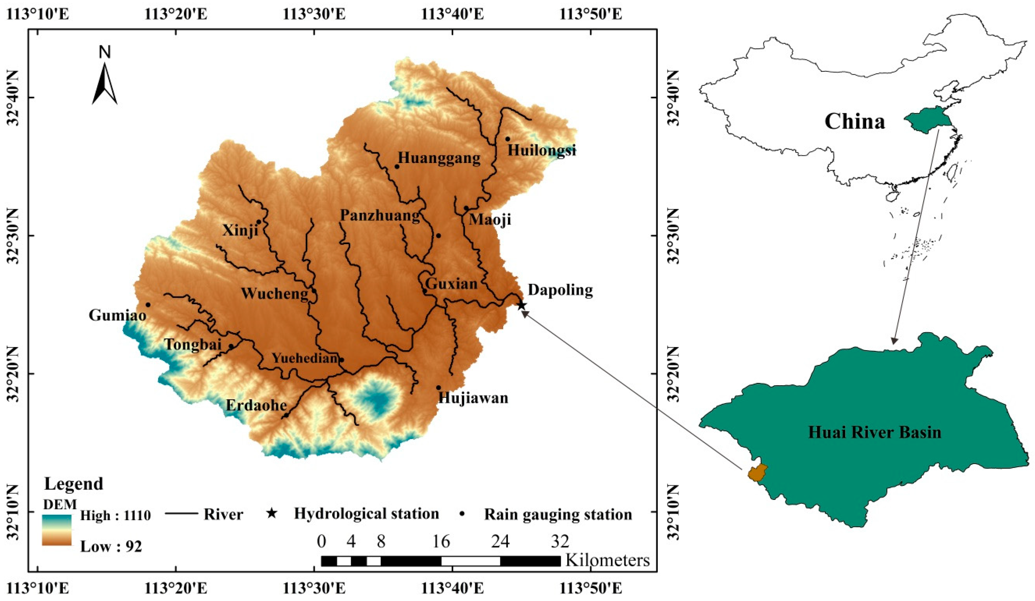
2.1. Study Area
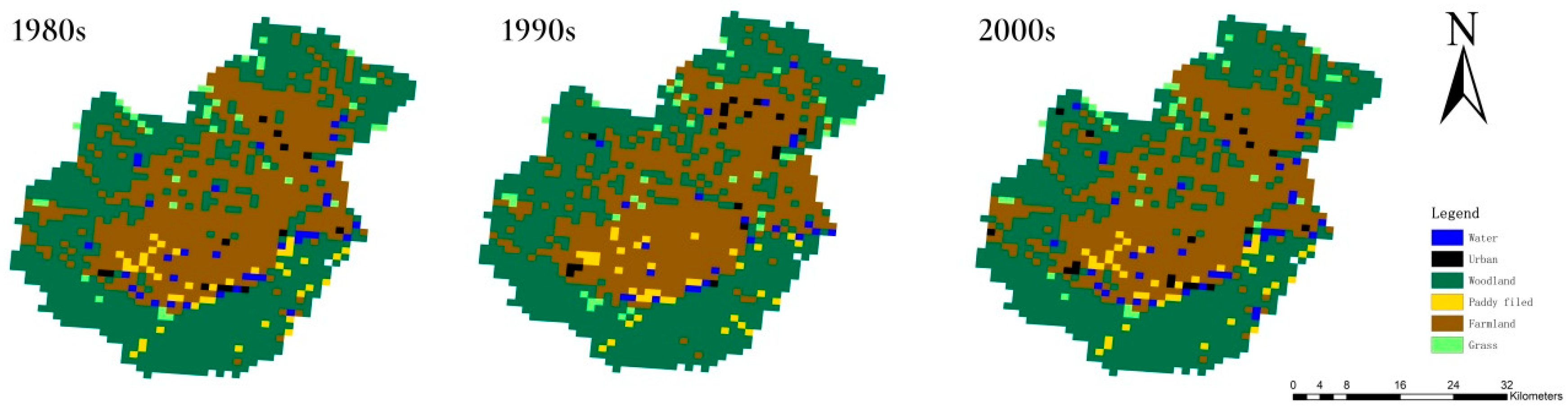
2.2. Land Use Data
3. Methods
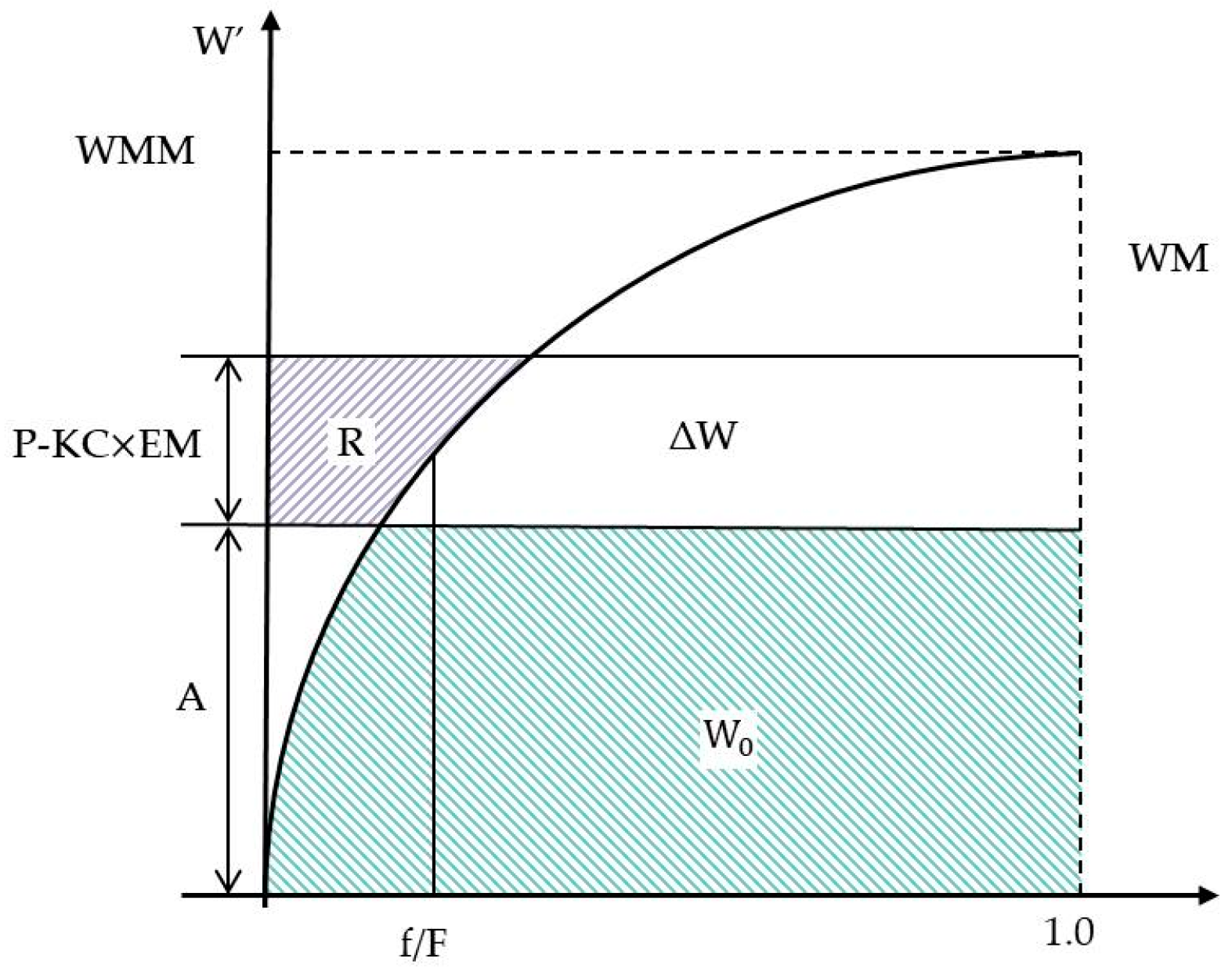
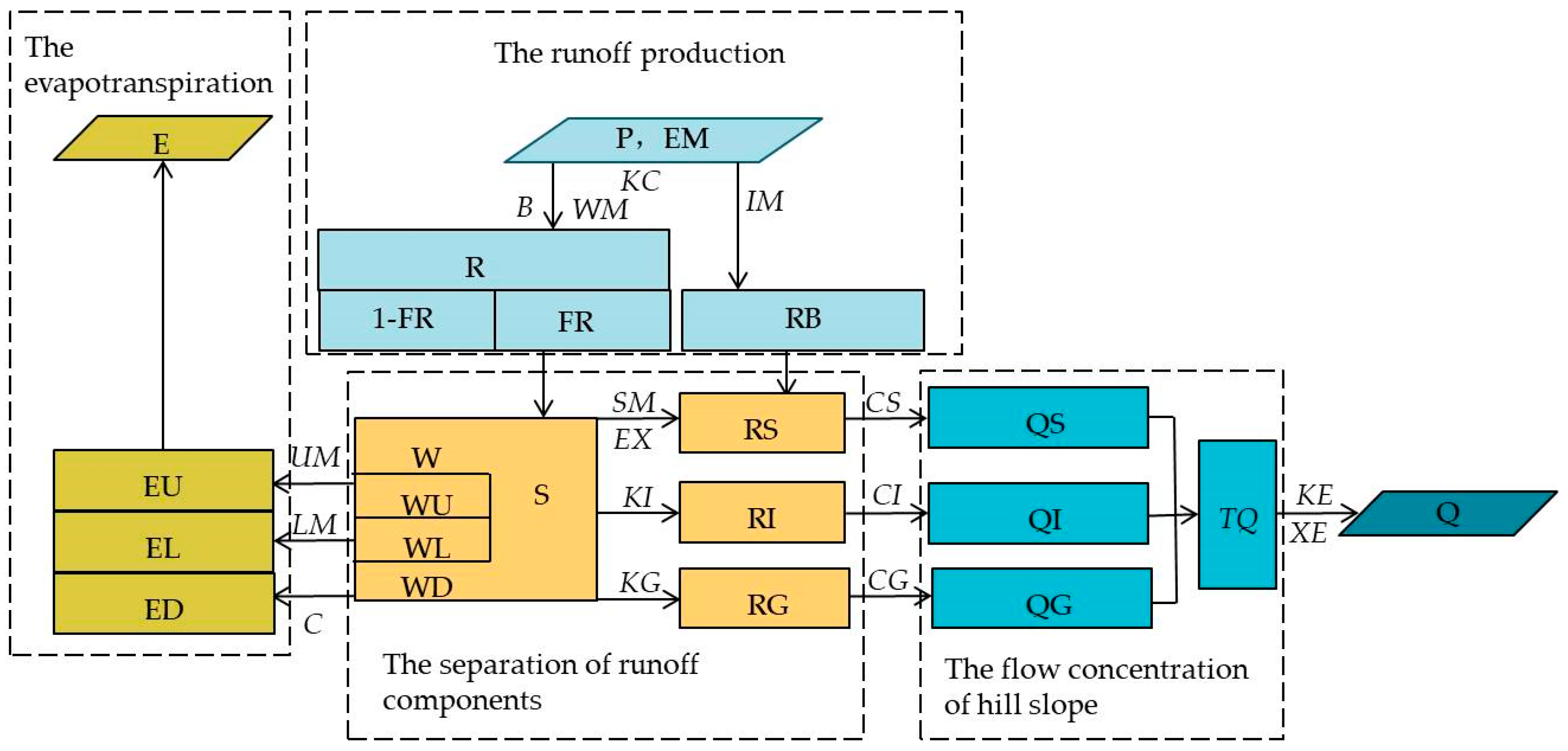
3.1. Xinanjiang Model
then R = P − KC × EM − WM + W0 + WM × [1 − (P − KC × EM + A)/WMM]1+B
3.2. Hydrology Data
3.2.1. Daily Model
3.2.2. Hourly Model
3.3. Data Processing
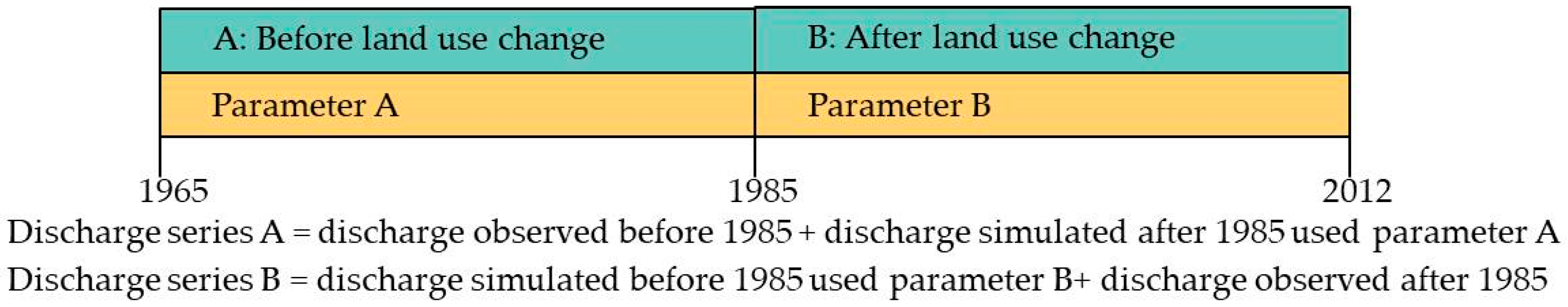
3.3.1. The Composing of Runoff Series
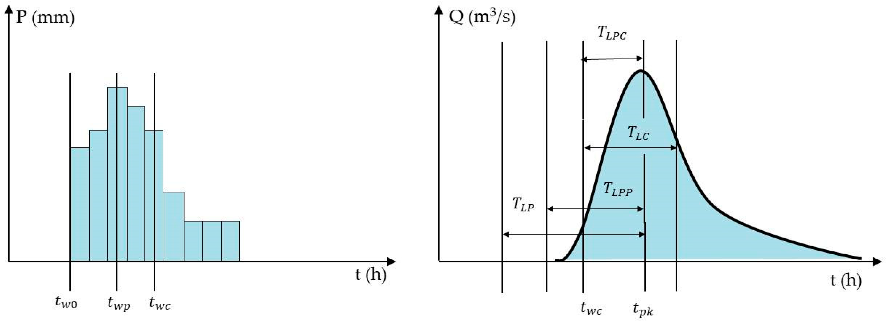
3.3.2. The Calculation of Lag Time
3.3.3. The Calculation of Rainfall–Runoff Relationship
4. Results and Discussion
4.1. Parameters Change of the Basin
4.2. Runoff Depth
4.3. Flood Peak
4.4. Kurtosis Coefficient
4.5. Rainfall–Runoff Relationship
4.6. Mean Lag Time Change of the Basin
5. Conclusions
Author Contributions
Funding
Acknowledgments
Conflicts of Interest
References
- Potter, K.W. Hydrological impacts of changing land management practices in a moderate-sized agricultural catchment. Water Resour. Res. 1991, 27, 845–855. [Google Scholar] [CrossRef]
- Vörösmarty, C.J.; Green, P.; Salisbury, J.; Lammers, R. Global water resources: Vulnerability from climate change and population growth. Science 2000, 289, 284–288. [Google Scholar] [CrossRef]
- Wan, R.; Yang, G. Progress in the Hydrological Impact and Flood Response of Watershed Land Use and Land Cover Change. J. Lake Sci. 2004, 16, 258–264. [Google Scholar] [CrossRef] [Green Version]
- Yang, T.; Zhang, Q.; Wang, W.; Yu, Z.; Chen, Y.D.; Lu, G.; Hao, Z.; Baron, A.; Zhao, C.; Chen, X.; et al. Review of Advances in Hydrologic Science in China in the Last Decades: Impact Study of Climate Change and Human Activities. J. Hydrol. Eng. 2013, 18, 1380–1384. [Google Scholar] [CrossRef]
- Calder, I.R.; Maidment, D.R. Maidment D. R. Handbook of Hydrology; McGraw-Hill: NewYork, NY, USA, 1993; Volume 13. [Google Scholar]
- Guo, Z.; Ma, Y.; Li, H.; Liu, W. Effect of Land Use Change on Runoff in the Liushahe Watershed, Xishuangbanna Southwest China. Res. Soil Water Conserv. 2006, 13, 139–142. [Google Scholar] [CrossRef]
- Yuan, F.; Ren, L.L.; Chen, X.; Chen, Y.D.; Xia, J.; Zhang, H. Evaluating the influence of land-cover change on catchment hydrology through the modified Xinanjiang model. In Proceedings of the International Association of Hydrological Sciences & the International Water Resources Association Conference, Guangzhou, China, 8–10 June 2006; pp. 167–174. [Google Scholar]
- Li, K.Y.; Coe, M.T.; Ramankutty, N.; Jong, R.D. Modeling the hydrological impact of land-use change in West Africa. J. Hydrol. 2007, 337, 258–268. [Google Scholar] [CrossRef]
- Liu, M.; Tian, H.; Chen, G.; Ren, W.; Zhang, C.; Liu, J. Effects of Land-Use and Land-Cover Change on Evapotranspiration and Water Yield in China During 1900-20001. J. Am. Water Resour. Assoc. 2010, 44, 1193–1207. [Google Scholar] [CrossRef]
- Yan, H.; Edwards, F.G. Effects of Land Use Change on Hydrologic Response at a Watershed Scale, Arkansas. J. Hydrol. Eng. 2013, 18, 1779–1785. [Google Scholar] [CrossRef]
- Zhang, H.; Huang, Q.; Zhang, Q.; Gu, L.; Chen, K.; Yu, Q. Changes in the long-term hydrological regimes and the impacts of human activities in the main Wei River, China. Hydrol. Sci. J. 2016, 61, 1054–1068. [Google Scholar] [CrossRef]
- Costa, M.H.; Botta, A.; Cardille, J.A. Effects of large-scale changes in land cover on the discharge of the Tocantins River, Southeastern Amazonia. J. Hydrol. 2003, 283, 206–217. [Google Scholar] [CrossRef]
- Wang, G.; Zhang, Y.; Liu, G.; Chen, L. Impact of land-use change on hydrological processes in the Maying River basin, China. Sci. China Ser. D Earth Sci. 2006, 49, 1098–1110. [Google Scholar] [CrossRef]
- Nazarnejad, H.; Solaimani, K.; Shahedi, K.; Sheikh, V. Evaluating hydrological response to land use change using the AGWA-GIS based hydrologic modeling tools. Int. J. Agric. Res. Rev. 2012, 2, 942–948. [Google Scholar] [CrossRef]
- Vanshaar, J.R.; Haddeland, I.; Lettenmaier, D.P. Effects of land-cover changes on the hydrological response of interior Columbia River basin forested catchments. Hydrol. Process. 2002, 16, 2499–2520. [Google Scholar] [CrossRef]
- Shi, P.; Zhang, Y.; Ren, Z.; Yu, Y.; Li, P.; Gong, J. Land-use changes and check dams reducing runoff and sediment yield on the Loess Plateau of China. Sci. Total Environ. 2019, 664, 984–994. [Google Scholar] [CrossRef]
- Keesstra, S.D.; Davis, J.; Masselink, R.H.; Casalí, J.; Peeters, E.T.; Dijksma, R. Coupling hysteresis analysis with sediment and hydrological connectivity in three agricultural catchments in Navarre, Spain. J. Soils Sediments 2019, 19, 1598–1612. [Google Scholar] [CrossRef]
- Abdulkareem, J.H.; Pradhan, B.; Sulaiman, W.N.A.; Jamil, N.R. Long-term runoff dynamics assessment measured through land use/cover (LULC) changes in a tropical complex catchment. Environ. Syst. Decis. 2019, 39, 16–33. [Google Scholar] [CrossRef]
- Brath, A.; Montanari, A.; Moretti, G. Assessing the effect on flood frequency of land use change via hydrological simulation (with uncertainty). J. Hydrol. 2006, 324, 141–153. [Google Scholar] [CrossRef]
- Fohrer, N.; Haverkamp, S.; Eckhardt, K.; Frede, H.-G. Hydrologic Response to land use changes on the catchment scale. Phys. Chem. Earth Part B Hydrol. Oceans Atmos. 2001, 26, 577–582. [Google Scholar] [CrossRef]
- De Roo, A.; Odijk, M.; Schmuck, G.; Koster, E.; Lucieer, A. Assessing the effects of land use changes on floods in the Meuse and Oder catchment. Phys. Chem. Earth Part B Hydrol. Oceans Atmos. 2001, 26, 593–599. [Google Scholar] [CrossRef]
- Mao, D.; Cherkauer, K.A. Impacts of land-use change on hydrologic responses in the Great Lakes region. J. Hydrol. 2009, 374, 71–82. [Google Scholar] [CrossRef]
- Hood, M.J.; Clausen, J.C.; Warner, G.S. Comparison of Stormwater Lag Times for Low Impact and Traditional Residential Development1. J. Am. Water Resour. Assoc. 2010, 43, 1036–1046. [Google Scholar] [CrossRef]
- Leopold, L.B. Lag times for small drainage basins. Catena 1991, 18, 157–171. [Google Scholar] [CrossRef]
- Watt, W.E.; Chow, K.C.A. A general expression for basin lag time. Can. J. Civ. Eng. 1985, 12, 294–300. [Google Scholar] [CrossRef]
- Loukas, A.; Quick, M. Physically-based estimation of lag time for forested mountainous watersheds. Int. Assoc. Sci. Hydrol. Bull. 1996, 41, 1–19. [Google Scholar] [CrossRef] [Green Version]
- Elsenbeer, H.; Vertessy, R.A. Stormflow generation and flowpath characteristics in an Amazonian rainforest catchment. Hydrol. Process. 2015, 14, 2367–2381. [Google Scholar] [CrossRef]
- Kang, I.S.; Park, J.I.; Singh, V.P. Effect of urbanization on runoff characteristics of the On-Cheon Stream watershed in Pusan, Korea. Hydrol. Process. 2015, 12, 351–363. [Google Scholar] [CrossRef]
- Talei, A.; Chua, L.H.C.; Quek, C. A novel application of a neuro-fuzzy computational technique in event-based rainfall-runoff modeling. Expert Syst. Appl. 2010, 37, 7456–7468. [Google Scholar] [CrossRef]
- Talei, A.; Chua, L.H.C. Influence of lag time on event-based rainfall–runoff modeling using the data driven approach. J. Hydrol. 2012, 438–439, 223–233. [Google Scholar] [CrossRef]
- Li, M.; Li, Q.; Cai, T.; Li, P.; Zou, Z. Modeling the effects of land-use change on runoff generation in the upper Huaihe River basin, China. In Proceedings of the 2012 International Symposium on Geomatics for Integrated Water Resource Management, Lanzhou, China, 19–21 October 2012; pp. 1–4. [Google Scholar]
- Chen, J.; Yu, Z.; Zhu, Y.; Yang, C. Relationship Between Land Use and Evapotranspiration-A Case Study of the Wudaogou Area in Huaihe River basin. Procedia Environ. Sci. 2011, 10, 491–498. [Google Scholar] [CrossRef] [Green Version]
- Li, Q.; Cai, T.; Yu, M.; Lu, G.; Xie, W.; Bai, X. Investigation into the impacts of land-use change on sediment yield characteristics in the upper Huaihe River basin, China. J. Hydrol. Eng. 2013, 18, 1464–1470. [Google Scholar] [CrossRef]
- Wen, H.; Li, Q.; Li, P.; Cai, T. Analysis of Impact of Land Use Change on Runoff Characteristics. Water Resour. Power 2013, 31, 12–14. [Google Scholar]
- Dong, J.; Chen, Q. Study on Relationship between Land Use Changes and Surface Water Quality in Western Regions of Xinyang City. Water Resour. Power 2010, 5, 29–32. [Google Scholar]
- Yu, L.; Xia, Z.; Li, Q.; Cai, T.; Guo, L.; Xie, W. Analysis of impact of land utilization change on non-point source pollution. Water Resour. Power 2012, 30, 100–102. [Google Scholar]
- Cai, T.; Li, Q.; Yu, M.; Lu, G.; Cheng, L.; Wei, X. Investigation into the impacts of land-use change on sediment yield characteristics in the upper Huaihe River basin, China. Phys. Chem. Earth Part B Hydrol. Oceans Atmos. 2012, 53–54, 1–9. [Google Scholar] [CrossRef]
- Qu, S.; Bao, W.; Shi, P.; Yu, Z.; Zhang, B. Evaluation of Runoff Responses to Land Use Changes and Land Cover Changes in the Upper Huaihe River Basin, China. J. Hydrol. Eng. 2012, 17, 800–806. [Google Scholar] [CrossRef]
- Zhang, Q.; Bao, W.M.; Chen, W.D.; Shen, D.D. Parameter Estimation Method Based on Parameter Function Surface to Evaluate Runoff Changes in Response to Land Use Changes in Dapoling Watershed. China Rural Water Hydropower 2015, 5, 49–52. [Google Scholar]
- Keesstra, S.; Temme, A.; Schoorl, J.; Visser, S. Evaluating the hydrological component of the new catchment-scale sediment delivery model LAPSUS-D. Geomorphology 2014, 212, 97–107. [Google Scholar] [CrossRef]
- Zhao, R. Watershed Hydrological Modeling; Water Conservancy and Electric Power Press: Beijing, China, 1984. [Google Scholar]
- Li, Z.; Yao, C.; Zhang, Y.; Qian, X.U.; Huang, Y. Study on grid-based Xinanjiang model. J. Hydroelectr. Eng. 2009, 28, 25–34. [Google Scholar] [CrossRef]
- Zhao, R.; Wang, P. The analysis of Xinanjiang model parameters. J. China Hydrol. 1988, 6, 4–11. [Google Scholar]


| Station Type | Station Code | Station Name | The Maximum Rainfall (mm) | The Maximum Discharge (m3/s) |
|---|---|---|---|---|
| Rainfall station | 82001 | Gumiao | 264.9 | - |
| 82002 | Tongbai | 365.1 | - | |
| 82003 | Erdaohe | 302.5 | - | |
| 82004 | Xinji | 326.5 | - | |
| 82005 | Wucheng | 275.2 | - | |
| 82006 | Yuehedian | 343.3 | - | |
| 82007 | Huanggang | 246.2 | - | |
| 82008 | Panzhuang | 245.2 | - | |
| 82009 | Guxian | 225.6 | - | |
| 82010 | Hujiawan | 324.2 | - | |
| 82011 | Huilongsi | 212.3 | - | |
| 82012 | Maoji | 211.6 | - | |
| Hydrology station | 82013 | Dapoling | 254.1 | 4200 |
| Mean annual precipitation of the basin (mm) | 918 | |||
| Mean annual runoff depth of the basin (mm) | 375 | |||
| Land Use | Proportion (%) | ||
|---|---|---|---|
| 1980s | 1990s | 2000s | |
| Water | 0.9 | 0.78 | 1.32 |
| Urban | 0.63 | 0.51 | 0.88 |
| Woodland | 38.55 | 40.69 | 38.06 |
| Paddy filed | 17.02 | 27.23 | 17.15 |
| Farmland | 41.85 | 30.38 | 41.81 |
| Grass | 0.57 | 0.06 | 0.54 |
| Symbol | Classify | Physical Meaning | Units | Range |
|---|---|---|---|---|
| KC | Calculation for evapotranspiration | The ratio of potential evapotranspiration to pan evaporation | - | 0.6–1.5 |
| UM | Tension water capacity of upper layer | mm | 5–20 | |
| LM | Tension water capacity of lower layer | mm | 60–90 | |
| C | The coefficient of deep evapotranspiration | - | 0.08–0.18 | |
| WM | Calculation for runoff producing | Areal mean tension water capacity | mm | 100–220 |
| B | The exponent of the tension water capacity curve | - | 0.1–0.4 | |
| SM | Calculation for separating water resources | Free water storage capacity | mm | 10–50 |
| EX | The exponent of the free water capacity curve | - | 1–1.5 | |
| KG | Outflow coefficient of free water storage to the groundwater flow | - | 0.2–0.6 | |
| KI | Outflow coefficient of free water storage to the interflow | - | 0.2–0.6 | |
| CS | Calculation for runoff concentration | Recession constant of surface water storage | - | 0.4–0.7 |
| CI | Recession constant of interflow storage | - | 0–0.9 | |
| CG | Recession constant of groundwater storage | - | 0.98–0.998 | |
| KE | Residence time of water | h | 0.5–1.5 | |
| XE | Muskingum coefficient | - | 0–0.5 |
| Symbol | Classify | Physical Meaning | Units |
|---|---|---|---|
| EM | Input | Pan evaporation of water surface | mm |
| E | Calculation for evapotranspiration | Total evaporation | mm |
| EU | Evaporation in upper soil layer | mm | |
| EL | Evaporation in lower soil layer | mm | |
| ED | Evaporation in deep soil layer | mm | |
| FR | Calculation for runoff producing | Fraction of runoff production area | - |
| IM | Fraction of impervious area | - | |
| RB | Runoff on impervious area | mm | |
| W | Calculation for separating water resources | Total tension water storage | mm |
| WU | Tension water storage in upper soil layer | mm | |
| WL | Tension water storage in lower soil layer | mm | |
| WD | Tension water storage in deep soil layer | mm | |
| S | Free water storage capacity in upper soil layer | mm | |
| RS | Surface runoff | mm | |
| RI | Interflow runoff | mm | |
| RG | Groundwater runoff | mm | |
| QS | Calculation for runoff concentration | Surface discharge | m3/s |
| QI | Interflow discharge | m3/s | |
| QG | Groundwater discharge | m3/s | |
| TQ | Total sub-basin inflow to the channel network | m3/s | |
| Q | Output | Basin discharge | m3/s |
| Flood Code | Calibration/Validation | Start Time | End Time | P | R | Qm |
|---|---|---|---|---|---|---|
| 31650708 | Calibration | 08/07/1965 17:00 | 13/07/1965 6:00 | 146.7 | 179.3 | 2720 |
| 31650713 * | Calibration | 13/07/1965 09:00 | 20/07/1965 8:00 | 79.2 | 68.3 | 1680 |
| 31650721 * | Calibration | 21/07/1965 6:00 | 31/07/1965 7:00 | 143.6 | 114.4 | 2260 |
| 31650803 * | Calibration | 03/08/1965 15:00 | 09/08/1965 7:00 | 73.7 | 97.4 | 1630 |
| 31670703 * | Calibration | 03/07/1967 12:00 | 09/07/1967 20:00 | 174.3 | 112.6 | 3080 |
| 31680712 | Calibration | 12/07/1968 12:00 | 30/07/1968 17:00 | 4.6 | 342.7 | 3680 |
| 31690422 * | Calibration | 22/04/1969 21:00 | 30/04/1969 16:00 | 91.4 | 72.6 | 1450 |
| 31710701 * | Calibration | 01/07/1971 1:00 | 05/07/1971 22:00 | 84.5 | 71.0 | 1810 |
| 31720619 | Calibration | 19/06/1972 8:00 | 24/06/1972 20:00 | 2.1 | 54.1 | 916 |
| 31730429 * | Calibration | 29/04/1973 11:00 | 03/05/1973 8:00 | 168.5 | 102.8 | 2110 |
| 31750805 * | Calibration | 05/08/1975 2:00 | 13/08/1975 3:00 | 354.5 | 314.4 | 4220 |
| 31770708 * | Calibration | 08/07/1977 18:00 | 14/07/1977 16:00 | 146.1 | 60.4 | 1100 |
| 31780624 * | Calibration | 24/06/1978 8:00 | 30/06/1978 6:00 | 222.1 | 87.6 | 1510 |
| 31790911 | Calibration | 11/09/1979 8:00 | 19/09/1979 8:00 | 167.7 | 101.5 | 984 |
| 31800623 * | Calibration | 23/06/1980 9:00 | 26/06/1980 15:00 | 170.1 | 103.1 | 1880 |
| 31810822 * | Calibration | 22/08/1981 21:00 | 26/08/1981 4:00 | 163.2 | 88.9 | 2020 |
| 31820811 * | validation | 11/08/1982 10:00 | 16/08/1982 19:00 | 136.4 | 107.6 | 1140 |
| 31840612 * | validation | 12/06/1984 12:00 | 18/06/1984 7:00 | 131.9 | 68.5 | 1600 |
| 31870605 * | validation | 05/06/1987 20:00 | 12/06/1987 7:00 | 124.4 | 75.2 | 1660 |
| 31890606 * | Calibration | 06/06/1989 18:00 | 12/06/1989 7:00 | 260.2 | 152.3 | 3280 |
| 31890806 | Calibration | 06/08/1989 14:00 | 16/08/1989 8:00 | 208.9 | 211.7 | 2460 |
| 31910612 | Calibration | 12/06/1991 12:00 | 29/06/1991 16:00 | 199 | 119.6 | 1420 |
| 31910706 * | Calibration | 06/07/1991 1:00 | 21/07/1991 8:00 | 121.1 | 79.3 | 1540 |
| 31910801 * | Calibration | 01/08/1991 0:00 | 23/08/1991 16:00 | 227.6 | 124.9 | 1540 |
| 31960628 * | Calibration | 28/06/1996 9:00 | 03/07/1996 8:00 | 164.2 | 51.1 | 1550 |
| 31970716 * | Calibration | 16/07/1997 23:00 | 25/07/1997 16:00 | 106.6 | 48.9 | 1220 |
| 31980701 * | Calibration | 01/07/1998 22:00 | 09/07/1998 8:00 | 88.9 | 68.8 | 1140 |
| 31980803 * | Calibration | 03/08/1998 2:00 | 20/08/1998 16:00 | 492.7 | 340.4 | 1730 |
| 31030717 * | Calibration | 17/07/2003 1:00 | 29/07/2003 0:00 | 159.6 | 72.9 | 1070 |
| 31050625 * | Calibration | 25/06/2005 18:00 | 05/07/2005 0:00 | 159.6 | 73 | 1920 |
| 31050709* | Calibration | 09/07/2005 2:00 | 12/07/2005 0:00 | 193.5 | 139.2 | 3520 |
| 31050829 * | Calibration | 29/08/2005 2:00 | 05/09/2005 16:00 | 169.4 | 111.6 | 2580 |
| 31070703 | Calibration | 03/07/2007 0:00 | 06/07/2007 21:00 | 130.4 | 68.4 | 1370 |
| 31070707 | Calibration | 07/07/2007 0:00 | 12/07/2007 16:00 | 125.9 | 78.4 | 1040 |
| 31090828 * | validation | 28/08/2009 13:00 | 07/09/2009 20:00 | 133.4 | 68.5 | 1140 |
| 31100715 | validation | 15/07/2010 8:00 | 21/07/2010 20:00 | 231.9 | 129 | 2020 |
| 31120907 * | validation | 07/09/2012 0:00 | 10/09/2012 20:00 | 155.4 | 37.8 | 966 |
| Parameters | Periods | |
|---|---|---|
| 1965−1985 | 1986−2009 | |
| KC | 0.77 | 0.95 |
| WM (mm) | 150 | 145 |
| UM (mm) | 20 | 20 |
| LM (mm) | 80 | 80 |
| B | 0.3 | 0.27 |
| C | 0.167 | 0.167 |
| SM (mm) | 13 | 13 |
| EX | 1.5 | 1.5 |
| KI | 0.42 | 0.50 |
| KG | 0.28 | 0.20 |
| CS | 0.55 | 0.56 |
| CI | 0.85 | 0.90 |
| CG | 0.993 | 0.994 |
| KE (h) | 1.4 | 1.2 |
| XE | 0.18 | 0.20 |
| Periods | Flood Code | Rsim (mm) | Robs (mm) | ER | Qmsim (m3/s) | Qmobs (m3/s) | EQ | DC |
|---|---|---|---|---|---|---|---|---|
| 1964–1985 | 31650708 | 152.2 | 179.3 | 0.151 | 3057 | 2720 | −0.124 | 0.898 |
| 31650713 | 58.1 | 68.3 | 0.149 | 1508 | 1680 | 0.102 | 0.97 | |
| 31650721 | 121.9 | 114.4 | −0.066 | 2011 | 2260 | 0.110 | 0.899 | |
| 31650803 | 75.2 | 97.4 | 0.228 | 1252 | 1630 | 0.232 | 0.816 | |
| 31670703 | 127.5 | 112.6 | −0.132 | 3311 | 3080 | −0.075 | 0.878 | |
| 31680712 | 361.4 | 342.7 | −0.055 | 3360 | 3680 | 0.087 | 0.984 | |
| 31690422 | 90.4 | 72.6 | −0.245 | 1143 | 1450 | 0.212 | 0.783 | |
| 31710701 | 79.8 | 71 | −0.124 | 1659 | 1810 | 0.083 | 0.896 | |
| 31720619 | 65.5 | 54.1 | −0.211 | 938 | 916 | −0.024 | 0.895 | |
| 31730429 | 116 | 102.8 | −0.128 | 1768 | 2110 | 0.162 | 0.864 | |
| 31750805 | 313.4 | 314.4 | 0.003 | 3837 | 4220 | 0.091 | 0.96 | |
| 31770708 | 70.2 | 60.4 | −0.162 | 1258 | 1100 | −0.144 | 0.938 | |
| 31780624 | 109.6 | 87.6 | −0.251 | 1606 | 1510 | −0.064 | 0.952 | |
| 31790911 | 114.7 | 101.5 | −0.130 | 979 | 984 | 0.005 | 0.862 | |
| 31800623 | 101.7 | 103.1 | 0.014 | 1736 | 1880 | 0.077 | 0.978 | |
| 31810822 | 100.7 | 88.9 | −0.133 | 1812 | 2020 | 0.103 | 0.922 | |
| 31820811 | 106.7 | 107.6 | 0.008 | 1221 | 1140 | −0.071 | 0.842 | |
| 31840612 | 68.5 | 68.5 | 0.000 | 1372 | 1600 | 0.143 | 0.973 | |
| 1986–2012 | 31870605 | 79 | 75.2 | −0.051 | 1580 | 1660 | 0.048 | 0.982 |
| 31890606 | 138.7 | 152.3 | 0.089 | 3054 | 3280 | 0.069 | 0.911 | |
| 31890806 | 153.8 | 211.7 | 0.274 | 2716 | 2460 | −0.104 | 0.665 | |
| 31910612 | 119 | 119.6 | 0.005 | 1240 | 1420 | 0.127 | 0.957 | |
| 31910706 | 76 | 79.3 | 0.042 | 1467 | 1540 | 0.047 | 0.968 | |
| 31910801 | 129.9 | 124.9 | −0.040 | 1655 | 1540 | −0.075 | 0.982 | |
| 31960628 | 63.2 | 51.1 | −0.237 | 1415 | 1550 | 0.087 | 0.863 | |
| 31970716 | 53.1 | 48.9 | −0.086 | 1237 | 1220 | −0.014 | 0.968 | |
| 31980701 | 68.7 | 68.8 | 0.001 | 1173 | 1140 | −0.029 | 0.895 | |
| 31980803 | 382.9 | 340.4 | −0.125 | 1591 | 1730 | 0.080 | 0.89 | |
| 31030717 | 77.1 | 72.9 | −0.058 | 988 | 1070 | 0.077 | 0.875 | |
| 31050625 | 66.9 | 73 | 0.084 | 1869 | 1920 | 0.027 | 0.994 | |
| 31050709 | 127.1 | 139.2 | 0.087 | 3237 | 3520 | 0.080 | 0.979 | |
| 31050829 | 111.7 | 111.6 | −0.001 | 2105 | 2580 | 0.184 | 0.903 | |
| 31070703 | 77.5 | 68.4 | −0.133 | 1117 | 1370 | 0.185 | 0.373 | |
| 31070707 | 86.4 | 78.4 | −0.102 | 912 | 1040 | 0.123 | -0.356 | |
| 31090828 | 81.7 | 68.5 | −0.193 | 1190 | 1140 | −0.044 | 0.888 | |
| 31100715 | 122.4 | 129 | 0.051 | 2046 | 2020 | −0.013 | 0.928 | |
| 31120907 | 49.2 | 37.8 | −0.302 | 990 | 966 | −0.025 | 0.545 |
| Statistics | R | Qm | Kr | |||
|---|---|---|---|---|---|---|
| Series A | Series B | Series A | Series B | Series A | Series B | |
| Maximum | 314.4 | 310.0 | 4220 | 3740 | 16.7 | 18.2 |
| Minimum | 39.9 | 37.7 | 892 | 966 | 2.4 | 2.2 |
| Variation range | 274.5 | 272.3 | 3328 | 2774 | 14.3 | 16.0 |
| Average | 87.16 | 92.49 | 1821 | 1916 | 7.50 | 7.66 |
| s | 49.90 | 50.04 | 795 | 774 | 3.70 | 3.99 |
| Rainfall (mm) | Statistics | R | Qm | Kr | |||
|---|---|---|---|---|---|---|---|
| Series A | Series B | Series A | Series B | Series A | Series B | ||
| <100 (7 events) | Maximum | 97.4 | 103.1 | 1680 | 2210 | 16.7 | 18.2 |
| Minimum | 45.6 | 48.9 | 1100 | 1070 | 3.6 | 4.2 | |
| Average | 66.1 | 70.0 | 1403 | 1440 | 9.6 | 9.3 | |
| 100–200 (23 events) | Maximum | 124.9 | 131.8 | 3630 | 3570 | 11.8 | 12.9 |
| Minimum | 39.9 | 37.7 | 892 | 966 | 2.4 | 2.2 | |
| Average | 82.2 | 87.3 | 1838 | 1999 | 6.6 | 7.2 | |
| >200 (7 events) | Maximum | 314.4 | 310.0 | 4220 | 3740 | 7.3 | 5.8 |
| Minimum | 87.6 | 101.1 | 1510 | 1680 | 5.1 | 4.9 | |
| Average | 176.8 | 187.8 | 2980 | 2900 | 5.9 | 5.2 | |
| Statistics | TLPC | TLC | TLP | TLPP | ||||
|---|---|---|---|---|---|---|---|---|
| Series A | Series B | Series A | Series B | Series A | Series B | Series A | Series B | |
| Maximum | 58.6 | 59.6 | 67.4 | 62.4 | 61 | 63 | 28 | 28 |
| Minimum | 2.9 | 1.5 | 6.6 | 6.9 | 10 | 10 | 4 | 4 |
| Variation range | 55.7 | 58.0 | 60.8 | 55.5 | 51.0 | 53.0 | 24.0 | 24.0 |
| Average | 11.92 | 11.67 | 25.28 | 25.10 | 17.00 | 22.57 | 11.11 | 10.86 |
| s | 9.97 | 10.21 | 11.01 | 11.73 | 11.51 | 11.68 | 4.69 | 4.86 |
| Rainfall (mm) | Statistics | TLPC | TLC | TLP | TLPP | ||||
|---|---|---|---|---|---|---|---|---|---|
| Series A | Series B | Series A | Series B | Series A | Series B | Series A | Series B | ||
| <100 (7 events) | Maximum | 15 | 16 | 41.4 | 47.4 | 39 | 35 | 15 | 14 |
| Minimum | 2.9 | 2.5 | 19.6 | 11.7 | 13 | 13 | 4 | 6 | |
| Average | 8.65 | 9.10 | 25.79 | 26.73 | 20.33 | 20.78 | 9.44 | 9.89 | |
| 100–200 (23 events) | Maximum | 58.6 | 59.6 | 67.4 | 62.4 | 34 | 32 | 28 | 28 |
| Minimum | 3.5 | 1.5 | 6.6 | 6.9 | 10 | 10 | 6 | 4 | |
| Average | 12.95 | 12.26 | 25.28 | 24.97 | 20.38 | 19.69 | 11.50 | 10.81 | |
| >200 (7 events) | Maximum | 19.4 | 19.8 | 28.5 | 25.2 | 61 | 63 | 18 | 20 |
| Minimum | 11.6 | 9.6 | 20.5 | 18.8 | 21 | 19 | 10 | 10 | |
| Average | 16.27 | 16.27 | 23.71 | 20.90 | 43.33 | 43.33 | 14.00 | 14.00 | |
© 2019 by the authors. Licensee MDPI, Basel, Switzerland. This article is an open access article distributed under the terms and conditions of the Creative Commons Attribution (CC BY) license (http://creativecommons.org/licenses/by/4.0/).
Share and Cite
Zhou, M.; Qu, S.; Chen, X.; Shi, P.; Xu, S.; Chen, H.; Zhou, H.; Gou, J. Impact Assessments of Rainfall–Runoff Characteristics Response Based on Land Use Change via Hydrological Simulation. Water 2019, 11, 866. https://doi.org/10.3390/w11040866
Zhou M, Qu S, Chen X, Shi P, Xu S, Chen H, Zhou H, Gou J. Impact Assessments of Rainfall–Runoff Characteristics Response Based on Land Use Change via Hydrological Simulation. Water. 2019; 11(4):866. https://doi.org/10.3390/w11040866
Chicago/Turabian StyleZhou, Minmin, Simin Qu, Xueqiu Chen, Peng Shi, Shijin Xu, Hongyu Chen, Huiyan Zhou, and Jianfeng Gou. 2019. "Impact Assessments of Rainfall–Runoff Characteristics Response Based on Land Use Change via Hydrological Simulation" Water 11, no. 4: 866. https://doi.org/10.3390/w11040866