A Conceptual Time-Varying Flood Resilience Index for Urban Areas: Munich City

Abstract

In response to the increased frequency and severity of urban flooding events, flood management strategies are moving away from flood proofing towards flood resilience. The term ‘flood resilience’ has been applied with different definitions. In this paper, it is referred to as the capacity to withstand adverse effects following flooding events and the ability to quickly recover to the original system performance before the event. This paper introduces a novel time-varying Flood Resilience Index (FRI) to quantify the resilience level of households. The introduced FRI includes: (a) Physical indicators from inundation modelling for considering the adverse effects during flooding events, and (b) social and economic indicators for estimating the recovery capacity of the district in returning to the original performance level. The district of Maxvorstadt in Munich city is used for demonstrating the FRI. The time-varying FRI provides a novel insight into indicator-based quantification methods of flood resilience for households in urban areas. It enables a timeline visualization of how a system responds during and after a flooding event.

1. Introduction

According to worldwide evidence of the last decades, the frequency and severity of extreme flooding events in urban areas are increasing [1,2,3]. The characteristics of an urban environment, such as the high portion of impervious area and increased population density, raise the vulnerability to flooding [4,5]. Traditional engineering measures face great challenges in providing sufficient flood protection when facing a more severe and frequent flooding condition [6,7]. In response, current flood protection strategies move away from measures to increase flood proofing towards flood resilience [8]. Various approaches to improve resilience to urban flooding have been proposed recently across different continents, such as the Best Management Practices (BMPs), Low Impact Development (LID), or Sustainable Urban Drainage Systems (SUDS). Furthermore, policies for improving public awareness of flood risk, advocating flood insurance, automated warning systems, etc. have also been advocated [9]. These approaches aim to mitigate the flooding impacts in cities by maintaining a high level of system performance during flooding events and facilitating the recovery stage of the system after flooding, i.e., its resilience. This study aims to develop a novel methodology to assess the flood resilience level of households within an urban area with time during and after a flooding event by incorporating physical, social, and economic factors.

There are numerous studies evaluating the benefits of flood resilience-enhancing strategies. However, many of them focus on flood impact reduction instead of resilience. Indeed, various flood impact assessment techniques have been formulated according to a wide diversity of research purposes, availability of data, and accessibility of resources [10]. On the contrary, the assessment of flood resilience faces many challenges, including its definition, dimensions used (e.g., social, economic, or physical aspects), and methods of quantification [11,12]. Nevertheless, there is a growing number of research projects and studies aiming at quantifying flood resilience using integrated [13] or multi-criteria [14] approaches, assessing climate variability [15] or the impact of infrastructure [16,17] while considering socioeconomic aspects [18]. Governance strategies for improving flood resilience have also been studied [19].

The study of resilience was originated in the field of ecology [20], where Holling defined it as the measure of the ability of an ecosystem to absorb changes and persist [21]. Since then, variations of the resilience concept started to emerge in different research fields. In the context of flood risk and flood management, various definitions have been introduced recently [22,23,24,25,26,27]. According to the literature, the definitions of flood resilience differ from each other. However, they generally comprise two major elements: 1. The coping capacity in the face of flooding, and 2. the recovery capacity after flooding. In this paper, these two major elements are adopted. Flood resilience is thus defined as “the capacity to withstand adverse effects following flooding events and the ability to quickly recover to the original system performance before the event”.

Resilience assessment can be used to evaluate flood risk management strategies at a city scale [28,29,30]. However, there still exists no consensus on how to measure flood resilience [31]. One commonly applied approach to quantify resilience is to utilize indicators that measure the characteristics of a system facing urban flooding. De Bruijn defined a set of indicators for flood resilience quantification, which covers three aspects: The amplitude of reaction, the graduality of the increase of the reaction with increasingly severe flood waves, and the recovery rate [32]. These three aspects describe the state of system performance when facing flooding events. In addition, the value of indicators reflects the physical, social, and economic factors regarding flood risk management. Batica and Gourbesville developed an urban flood vulnerability and resilience assessment tool with indicators providing a comprehensive overview of vulnerability and resilience of a city and its community [33]. An index is proposed to describe resilience level by assigning grades (0 to 5) to different indicators according to the availability levels to various urban services when facing a 100-year flooding event. Mugume et al. quantified the resilience of urban drainage systems in the UK by applying the utility performance function combined with the depth–damage data for residential properties that relates the overall performance of a drainage system to flood depths [25]. Analogously, Lee and Kim proposed a resilience index for urban drainage systems in Korea based on flooding damage that resulted from damage functions calculated by multi-dimensional flood damage analysis [34]. However, both studies on urban drainage systems lack socioeconomic aspects when estimating resilience. Bertilsson and Wiklund developed a spatialized index to measure and visualize flood resilience changes in an urban area of Rio [35], incorporating five dimensions: Flood level, exposed population, susceptibility, material recovery, and flood duration.

Despite the already existing studies on flood resilience quantification, there is a lack of methods for assessing how a system’s resilience level is affected during and after flooding. As discussed, most existing studies are not time-dependent. Therefore, the aim of this study is to propose a time-dependent method for quantifying flood resilience of households in urban areas.

Section 2 introduces the study area of Maxvorstadt in Munich city. In Section 3, the structure of the Flood Resilience Index (FRI) and the computation of each parameter are explained in detail. In Section 4 and Section 5, the inundation and FRI modelling results for Maxvorstadt as well as the sensitivity analysis of the applied reference parameters are provided and discussed. Finally, in Section 6, the conclusion highlights the main advantage and limitation of the proposed FRI method and consideration for future work.

2. Study Area and Data

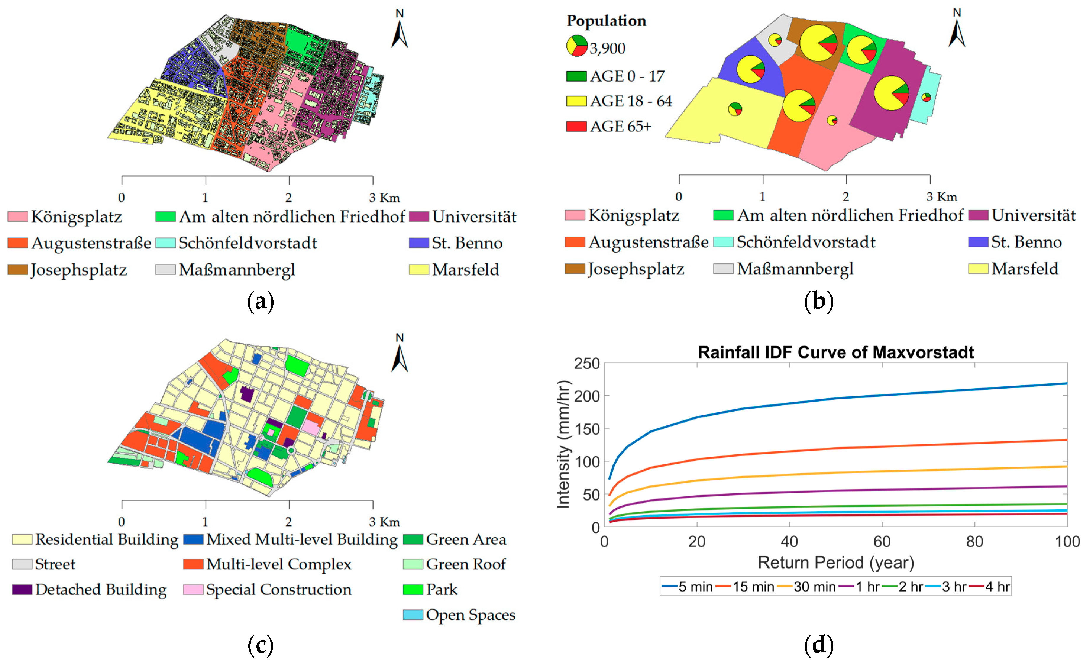
The study area of Maxvorstadt is one of the 25 boroughs within Munich city, located at the city center. The borough contains an area of 429.79 ha, and is composed of 69% of buildings, 7% of recreation area, and 24% of road surface [36]. The geographical range of the study site is trimmed alongside the roads at the boundary of the administrative area of Maxvorstadt to exclude buildings crossing over multiple boroughs. Maxvorstadt consists of nine districts, which are Königsplatz, Augustenstraße, St. Benno, Marsfeld, Josephsplatz, Am alten nördlichen Friedhof, Universität, Schönfeldvorstadt, and Maßmannbergl (see Figure 1a).

Table 1. The amount of buildings and area for each district within Maxvorstadt.

District Name	N 2	% of Total N	Area [ha]	% of Total Area	D 3
Königsplatz	417	7.48%	62.43	16.83%	6.68
Augustenstraße	1196	21.46%	51.88	13.98%	23.05
St. Benno	620	11.13%	32.52	8.76%	19.07
Marsfeld	630	11.30%	75.96	20.47%	8.29
Josephsplatz	787	14.12%	31.30	8.44%	25.14
Am a- n- Friedhof 1	437	7.84%	21.35	5.75%	20.47
Universität	1195	21.44%	64.84	17.48%	18.43
Schönfeldvorstadt	168	3.01%	13.91	3.75%	12.08
Maßmannbergl	123	2.21%	16.83	4.54%	7.31
Maxvorstadt	5573	100%	371.02	100%	15.02

¹ Am alten nördlichen Friedhof. ² Number of buildings. ³ Building density [building/ha].

shows the number of buildings and area within each district. Figure 1b illustrates the population and age distribution of each district. The population of Maxvorstadt lies mainly between 20 to 30 years old [36]. Like other urban areas, the majority of the surface area within Maxvorstadt is sealed. However, there are parks, cemeteries, and lawns composing 7% of the total area as green spaces. Furthermore, some buildings are constructed with green roofs or roof-top gardens, making up more green surface areas. Figure 1c shows the land use map of the study site.

The average yearly precipitation from 1981 to 2010 of Munich City was 944 mm [37]. Regarding rainfall events, the German Meteorological Office (Deutscher Wetterdienst, DWD) provides a dataset storing grids of return periods of heavy rainfall over Germany (Koordinierte Starkniederschlagsregionalisierung und -auswertung des DWD, KOSTRA-DWD). The dataset contains statistical rainfall intensity values as a function of the duration and return period. It is often applied to assess damages caused by severe design rainfalls with regard to their return period [38]. This paper applies the latest version of the dataset, the KOSTRA-DWD-2010R, which encompasses the time period from 1951 to 2010 and focuses on the 15 min duration rainfall events for various return periods (see Figure 1d).

3. Methods

3.1. Time-Varying Flood Resilience Index: FRI

3.1.1. Structure of the Flood Resilience Index

A time-varying Flood Resilience Index (FRI) is developed to quantify the resilience level of households in Maxvorstadt, ranging from 0 to 1 as the minimum and maximum value, respectively. The FRI quantifies the capacity to withstand the adverse effects during flooding and the ability to quickly recover from them at each timestep. Indicators reflecting physical, social, and economic dimensions are considered for computing the FRI.

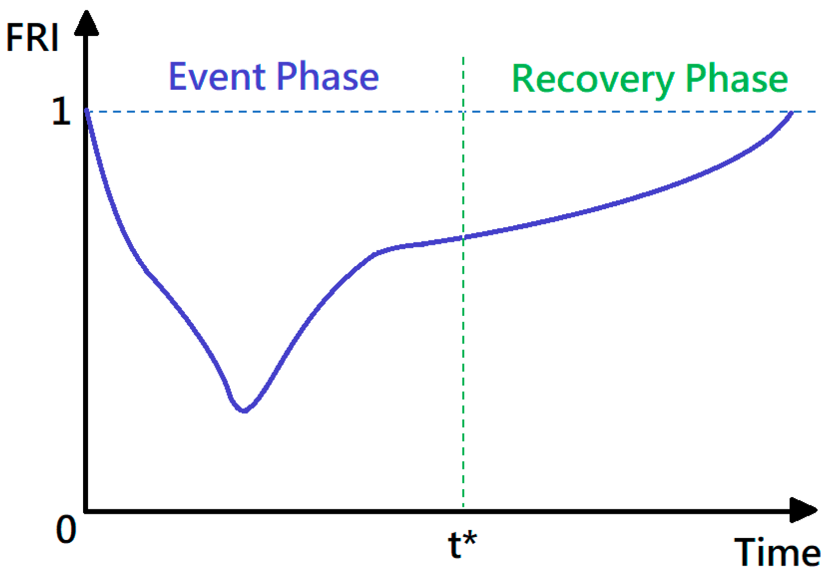
The evaluation of the FRI is split into two phases: The event phase and the recovery phase, depending on the indoor water depth (see Figure 2). In the event phase, physical indicators from flood modelling, i.e., water depth, accumulated water depth, flooding duration, and water accumulation rate are incorporated to assess the flooding impacts. It is assumed that after each flooding event, when the indoor water depth recedes to zero, the recovery phase is initiated. Aside from the physical indicators, social indicators (i.e., percentage of households with children and percentage of elderly population) and economic indicators (i.e., household income) are considered to evaluate the recovery capacity, which facilitates the system to bounce back to the original performance level before flooding (FRI = 1). A description of each indicator and its computation will be introduced in the following section.

3.1.2. Event Phase Indicators

When the indoor water depth is larger than zero, it is considered as an event phase. In this case, four physical indicators are considered for calculating the FRI: Water depth ($I_h\left(t\right)$), accumulated water depth ($I_{AWD}\left(t\right)$), flooding duration ($I_D\left(t\right)$), and water accumulation rate ($I_{WAR}\left(t\right)$).

The water depth indicator indicates the severity of flooding at each timestep. The higher the water depth is, the more a household, human, and items are affected, and thus the less resilient the system becomes. A value is assigned to a reference parameter, which indicates the maximum water depth that the building can withstand ($h_{ref}$ [m]). The resilience level decreases as the indoor water depth rises, and once the indoor water depth exceeds the reference parameter, the water depth indicator becomes zero. Equation (1) computes the water depth indicator ($I_h\left(t\right)$), where variable $h_{in}\left(t\right)$ [m] is the indoor water depth at time $t$. The reference parameter of water depth $h_{ref}$ [m] is assigned a value of 0.5 m.

$$I_h\left(t\right)=\{\begin{array}{c}1-\frac{h_{in}\left(t\right)}{h_{ref}},if{h}_{ref}\ge h_{in}\left(t\right)\\ 0,otherwise\end{array}$$

(1)

The water depth indicator shows the severity of the flooding at a certain timestep. However, it is also important to investigate the full scope of the impact that the flooding event has caused. Hence, the accumulated water depth indicator is developed. A reference parameter is inserted, stating the maximum accumulated water depth that the building can withstand ($AW{D}_{ref}$ [m]). Equation (2) calculates the accumulated water depth indicator ($I_{AWD}\left(t\right)$) at every time step (every 10 s), where $t_s$ [s] is the starting time of the flooding event. $AW{D}_{ref}$ [m] is assigned a value of 3 m.

$$I_{AWD}\left(t\right)=\{\begin{array}{l}1-\frac{{{\displaystyle \sum }}_{t_s}^t{h}_{in}\left(t\right)}{AW{D}_{ref}},ifAW{D}_{ref}\ge {\displaystyle {\displaystyle \sum }_{t_s}^t}{h}_{in}\left(t\right)\\ 0,otherwise\end{array}$$

(2)

The duration of the flooding event plays an important role in evaluating the FRI. The longer the flood lasts, the higher damage it will cause. Young points out several impacts that the long-lasting floods could bring to human health, including toxic chemical exposure, growing mold causing respiratory problems, and mosquitos carrying a variety of diseases [39]. In addition, financial damage, social losses, and impacted level of well-being, such as breakdowns of factories and transportations, can have a large impact on the society leading to a lower resilience level [40,41,42]. These adverse effects become more significant when the flood duration increases. The flooding duration indicator ($I_D\left(t\right)$) is calculated by Equation (3), where $D\left(t\right)$ [min] stands for the flooding duration until time $t$. The reference parameter $D_{ref}$ [min] presents the maximum flooding duration that a household can withstand, which is assigned a value of 800 min.

$$I_D\left(t\right)=\{\begin{array}{c}1-\frac{D\left(t\right)}{D_{ref}},if{D}_{ref}\ge D\left(t\right)\\ 0,otherwise\end{array}$$

(3)

The rising rate of the floodwater is one of the most influential factors which determines the damage magnitude caused by flooding events. For instance, the evacuation procedure should be executed within a limited time span. If the rising rate of the floodwater is high, the evacuation might be incomplete or executed with a reduced efficiency. Facilities with higher vulnerability to fast-rising water, such as schools and nursing homes, will then have a much lower resilience level. In this paper, a water accumulation rate indicator is considered at the rising stage of a flood. Equation (4) computes the water accumulation rate indicator ($I_{WAR}\left(t\right)$), where $r_{rise}\left(t\right)$ [cm/min] stands for the water rising rate during time $t$ and $t-1$. The reference parameter $WA{R}_{ref}$ [cm/min] represents the highest water rising rate that can be tolerated, which is assigned a value of 5 cm/min.

$$I_{WAR}\left(t\right)=\{\begin{array}{l}1-\frac{r_{rise}\left(t\right)}{WA{R}_{ref}},ifWA{R}_{ref}\ge r_{rise}\left(t\right)\\ 0,otherwise\end{array}$$

(4)

3.1.3. Recovery Phase Indicators

When the indoor water depth recedes to zero, the recovery phase is initiated. In this case, not only the physical indicators, but the social and economic ones are applied for calculating a recovery factor in order to enhance the FRI after flooding. The four physical indicators include flood severity ($I_{fs}$), total flooding depth ($I_{TFD}$), total flooding time ($I_{TFT}$), and maximum water accumulation rate ($I_{WRAmax}$). The two social indicators are households with children ($I_C$) and elderly population ($I_E$). The economic indicator is household income ($I_I$). Seven indicators in total comprise the recovery factor, which is a product of seven exponential terms.

The concepts of the physical indicators in the recovery phase are similar to those in the event phase. However, there is a slight difference at the evaluation time frame. Instead of taking values for the numerators at current time steps, the maximum or the accumulated values during the previous event phase are considered. For flood severity ($I_{fs}$) and maximum water accumulation rate indicators ($I_{WARmax}$), the maximum value of the indoor water depth and the water accumulation rate within the previous event phase are considered, respectively. As for total flooding depth ($I_{TFD}$) and total flooding time indicators ($I_{TFT}$), a cumulative value of the indoor water depth and total flooding duration within the previous event phase are considered. Equations (5)–(8) show the calculation of the four physical indicators, respectively. Variables $t_s$ and $t_e$ represent the starting and ending timesteps of flooding in the previous event phase.

$$I_{fs}=\{\begin{array}{l}{e}^{\left(1-\frac{\underset{t\in \left[t_s,t_e\right]}{\max }{h}_{in}\left(t\right)}{h_{ref}}\right)},if{h}_{ref}\ge \underset{t\in \left[t_s,t_e\right]}{max}{h}_{in}\left(t\right)\\ 1,otherwise\end{array}$$

(5)

$$I_{TFD}=\{\begin{array}{l}{e}^{\left(1-\frac{{{\displaystyle \sum }}_{t_s}^{t_e}{h}_{in}\left(t\right)}{AW{D}_{ref}}\right)},ifAW{D}_{ref}\ge {\displaystyle {\displaystyle \sum }_{t_s}^{t_e}}{h}_{in}\left(t\right)\\ 1,otherwise\end{array}$$

(6)

$$I_{TFT}=\{\begin{array}{l}{e}^{\left(1-\frac{D\left(t_e\right)}{D_{ref}}\right)},if{D}_{ref}\ge D\left(t_e\right)\\ 1,otherwise\end{array}$$

(7)

$$I_{WARmax}=\{\begin{array}{l}{e}^{\left(1-\frac{\underset{t\in \left[t_s,t_e\right]}{\max }{r}_{rise}\left(t\right)}{WA{R}_{ref}}\right)},ifWA{R}_{ref}\ge \underset{t\in \left[t_s,t_e\right]}{max}{r}_{rise}\left(t\right)\\ 1,otherwise\end{array}$$

(8)

Social and economic indicators are assigned to evaluate the recovery capacity from flooding for each household according to different districts within Maxvorstadt. The demographic and social–economic characteristics, such as race, gender, age, and income are principal drivers of a population’s ability to recover from damaging flooding events [43,44,45]. The more children and elderly people within a district, the higher vulnerability to flooding and lower recovery strength the community has. Equations (9) and (10) show the calculation for the indicators of households with children ($I_C$) and elderly population ($I_E$), respectively. Furthermore, household income straightforwardly reflects the recovery strength from a flooding event. The more a household earns, the easier and faster it can recover from flooding by repairing or replacing the damaged goods. Equation (11) computes the income indicator ($I_I$).

$$I_C=\{\begin{array}{c}{e}^{\left(1-\frac{C}{C_{ref}}\right)},if{C}_{ref}\ge C\\ 1,otherwise\end{array}$$

(9)

$$I_E=\{\begin{array}{c}{e}^{\left(1-\frac{E}{E_{ref}}\right)},if{E}_{ref}\ge E\\ 1,otherwise\end{array}$$

(10)

$$I_I=\{\begin{array}{c}{e}^{\frac{I}{I_{ref}}},if{I}_{ref}\ge I\\ e^1,otherwise\end{array}$$

(11)

$C$ [%] and $E$ [%] stand for the percentage of households with children and elderly population, respectively, in the district that the household is seated in. Reference parameters, $C_{ref}$ [%] and $E_{ref}$ [%], are assigned values 20% and 12%, respectively, which provide the thresholds that the recovery capacity decreases as $C$ and $E$ increase. $I$ [€] represents the annual household income, and reference parameter $I_{ref}$ [€], assigned 80,000€, represents the threshold that the recovery capacity increases as $I$ increases.

3.1.4. Time Series of the Flood Resilience Index

Once the indicators for evaluating FRI in the event phase and the recovery factor in the recovery phase are calculated, the time series of FRI can be computed. Like the calculation of the indicators, the computation of the FRI time series should be divided into event and recovery phases.

In the event phase, the calculated indicators of water depth ($I_h\left(t\right)$), accumulated water depth ($I_{AWD}\left(t\right)$), flooding duration ($I_D\left(t\right)$), and water accumulation rate ($I_{WAR}\left(t\right)$) are applied to evaluate the FRI at time $t$ following Equation (12). $WF$ stands for the weighting factor for each indicator, which determines the relative level of significance among the indicators. $W{F}_h$, $W{F}_{AWD}$, $W{F}_D$, and $W{F}_{WAR}$ are assigned values of 3, 1, 3, and 2, respectively. $t_s$ and $t_e$ represent the starting and ending timesteps of flooding in the event phase.

$$\begin{array}{c}FRI\left(t\right)=\hfill \\ \left[\frac{W{F}_h·I_h\left(tt\right)+W{F}_{AWD}·I_{AWD}\left(t\right)+W{F}_D·I_D\left(t\right)+W{F}_{WAR}·I_{WAR}\left(t\right)}{\left(W{F}_h+W{F}_{AWD}+W{F}_D+W{F}_{WAR}\right)}\right]\hfill \\ ift\in \left[t_s,t_e\right]\hfill \end{array}$$

(12)

In the recovery phase, a recovery factor ($RF$) is calculated based on the physical characteristics of flooding in the previous event phase, and the social and economic indicator values of a household and its corresponding district. Equation (13) computes the recovery factor, applying the indicators of flood severity ($I_{fs}$), total flooding depth ($I_{TFD}$), total flooding time ($I_{TFT}$), maximum water accumulation rate ($I_{WARmax}$), households with children ($I_C$), elderly population ($I_E$), and household income ($I_I$). Weighting factors $W{F}_{fs}$, $W{F}_{TFD}$, $W{F}_{TFT}$, $W{F}_{WARmax}$, $W{F}_C$, $W{F}_E$ and $W{F}_I$ are assigned values of 3, 1, 2, 1, 1, 2, and 3, respectively. A value of 0.001 is assigned as a scaling constant. At last, the FRI at time t is computed as the product of the recovery factor and the FRI at the previous timestep t − 1 (see Equation (14)). Note that the recovery phase will last until the FRI value reaches 1.

$$\begin{array}{c}x=\left\{fs,TFD,TFT,WARmax,C,E,I\right\}\hfill \\ RF={\left[\prod {\left(I_x\right)}^{W{F}_x}\right]}^{\frac{0.001}{\sum W{F}_x}}\hfill \end{array}$$

(13)

$$FRI\left(t\right)=FRI\left(t-1\right)\times RF,ift\notin \left[t_s,t_e\right]$$

(14)

3.2. Indoor Water Depth Modelling

The indoor water depth modelling can be conducted based on a one-way coupling computation given the inundation modelling result from the 2D surface runoff model Parallel Diffusive Wave (P-DWave). It is assumed that floodwater flows into the buildings through doors with known location and it follows the fluid mechanics of discharge over a rectangular weir. Furthermore, the width of the door for every building is assumed to be 75 cm.

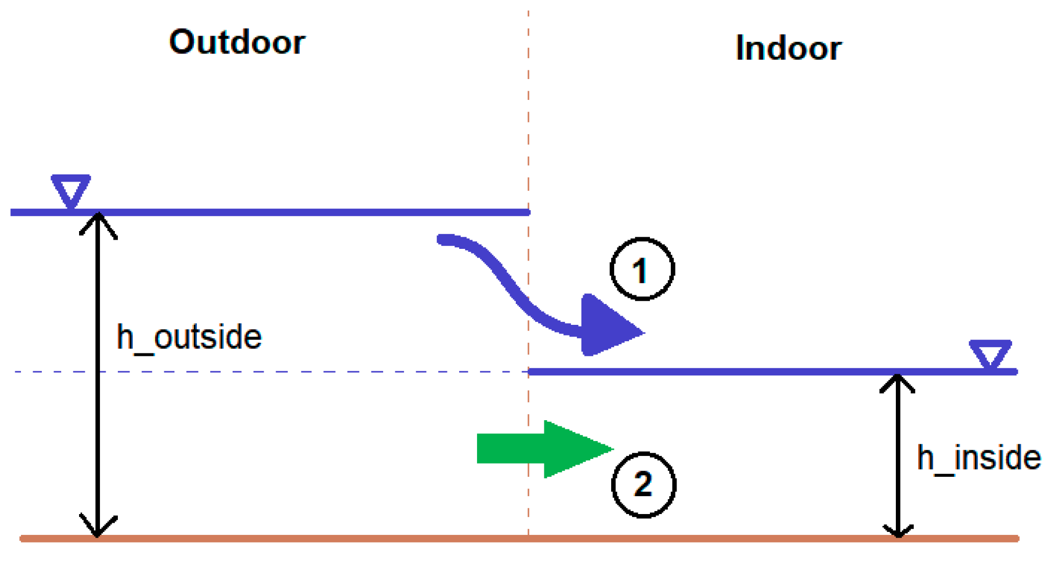
Figure 3 diagrammatizes the flow dynamic of water coming into the building. The flow should be analyzed by the upper and lower portion. At the upper portion of the flow, the income discharge is calculated by Equation (15), which describes a free discharge under a head of water equal to $\left(h_{out}-h_{\mathrm{in}}\right)$. At the lower portion of the flow, the income discharge is calculated by Equation (16), which describes a submerged discharge under a head of water equal to $h_{\mathrm{in}}$. $Q_u$ [m³/s] and $Q_l$ [m³/s] represent the upper and lower portions of the discharge, respectively. $C_d$ stands for the discharge coefficient, which in this case is assigned a value of 1. $L$ (m) is the width of the door, assumed to be 0.75 m. Variable $h_{out}$ (m) and $h_{in}$ (m) represent the outdoor and indoor water level, respectively.

$$Q_u=\frac{2}{3}{C}_d\times L\times \sqrt{2g}\times {\left(h_{out}-h_{in}\right)}^{\frac{3}{2}}$$

(15)

$$Q_l=C_d\times L\times h_{in}\times \sqrt{2g\times \left(h_{out}-h_{in}\right)}$$

(16)

The total discharge, $Q_t$ [m³/s], is calculated by summing up $Q_u$ and $Q_l$. When the outdoor water level recedes, $h_{outside}$ becomes lower than $h_{in}$, hence, $Q_u$ and $Q_l$ become negative. From that point, the water is flowing outwards, shown as a negative value of $Q_t$. After $Q_t\left(t\right)$ is calculated at time $t$, the water volume entering or exiting the building at time $t$, $V_{flux}\left(t\right)$ [m³], can be calculated by Equation (17). Then, the water volume inside the house at time $t$, $V\left(t\right)$ [m³], can be computed by Equation (18). At last, the indoor water depth at time $t$, $h_{in}\left(t\right)$ [m], is computed by Equation (19). $\Delta t$ [s] represents the computation time interval, which in this case is 10 s. $Area$ [m²] stands for the building area.

$$V_{flux}\left(t\right)=Q_t\left(t\right)·\Delta t$$

(17)

$$V\left(t\right)=V\left(t-1\right)+V_{flux}\left(t\right)$$

(18)

$$h_{in}\left(t\right)=\frac{V\left(t\right)}{Area}$$

(19)

3.3. Parallel Diffusive Wave Model: P-DWave

The Parallel Diffusive Wave Model, P-DWave, is the surface runoff model applied for flood inundation modelling in this study. It is a first-order finite volume explicit discretization scheme that takes the conservative form of the 2D Shallow Water Equations into account and neglects the inertial terms (see Equations (20) and (21)). $h$ is the water depth [m] and $t$ is the time [s]. Velocity is defined by $u^2=u_x{}^2+u_y{}^2$. $u={\left[\begin{array}{cc}{u}_x& u_y\end{array}\right]}^T$ stands for the depth-averaged flow velocity vector [-], in which $u_x$ is the flow velocity in the x direction [m/s] and $u_y$ is the flow velocity in the y direction [m/s]. $R$ represents the source/sink term (e.g., rainfall, inflow, surcharge, drainage [m/s]). $z$ is the bed elevation [m]. The bed friction is approximated by Manning’s formula (Equation (22)), in which $S_f={\left[\begin{array}{cc}{S}_{fx}& S_{fy}\end{array}\right]}^T$ stands for the bed friction vector [-]. $S_{fx}$ is the bed friction slope in the x direction [-] and $S_{fy}$ is the bed friction slope in the y direction [-]. $n$ is the Manning’s roughness coefficient [s/m1/3]. The modulus of the depth-averaged flow velocity vector is given by Equation (23), where $S_{wx}=d\left(h+z\right)/dx$ is the water level gradient in the x direction [-] and $S_{wy}=d\left(h+z\right)/dy$ is the water level gradient in the y direction [-]. Further details of the P-DWave model can be found elsewhere [46]. Note that neither the sewer system nor the infiltration processes are considered in this study. As such, not all water could be drained from the surface and the event phase could not be considered complete. Therefore, in order to enable the start of the recovery phase, we assume that the outdoor water depths after the end of the 60-min simulation time return automatically to zero. The one-way coupling indoor water depth simulation for each building is then conducted following this assumption.

$$\frac{dh}{dt}+\nabla \left(uh\right)=R$$

(20)

$$g\nabla \left(h+z\right)=g{S}_f$$

(21)

$$\left[\begin{array}{c}{S}_{fx}\\ S_{fy}\end{array}\right]=\left[\begin{array}{c}\frac{n^2\left|u\right|u_x}{h^{\raisebox{1ex}{$4$}\!\left/ \!\raisebox{-1ex}{$3$}\right.}}\\ \frac{n^2\left|u\right|u_y}{h^{\raisebox{1ex}{$4$}\!\left/ \!\raisebox{-1ex}{$3$}\right.}}\end{array}\right]$$

(22)

$$\left|u\right|=\frac{h^{\raisebox{1ex}{$2$}\!\left/ \!\raisebox{-1ex}{$3$}\right.}{\left(S_{wx}{}^2+S_{wy}{}^2\right)}^{\raisebox{1ex}{$1$}\!\left/ \!\raisebox{-1ex}{$4$}\right.}}{n}$$

(23)

4. Results

4.1. Flood Inundation Modelling

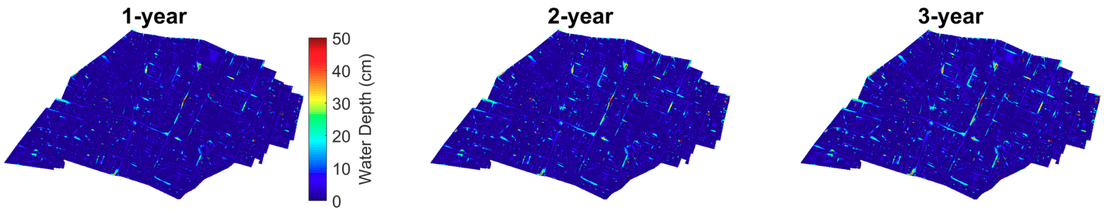
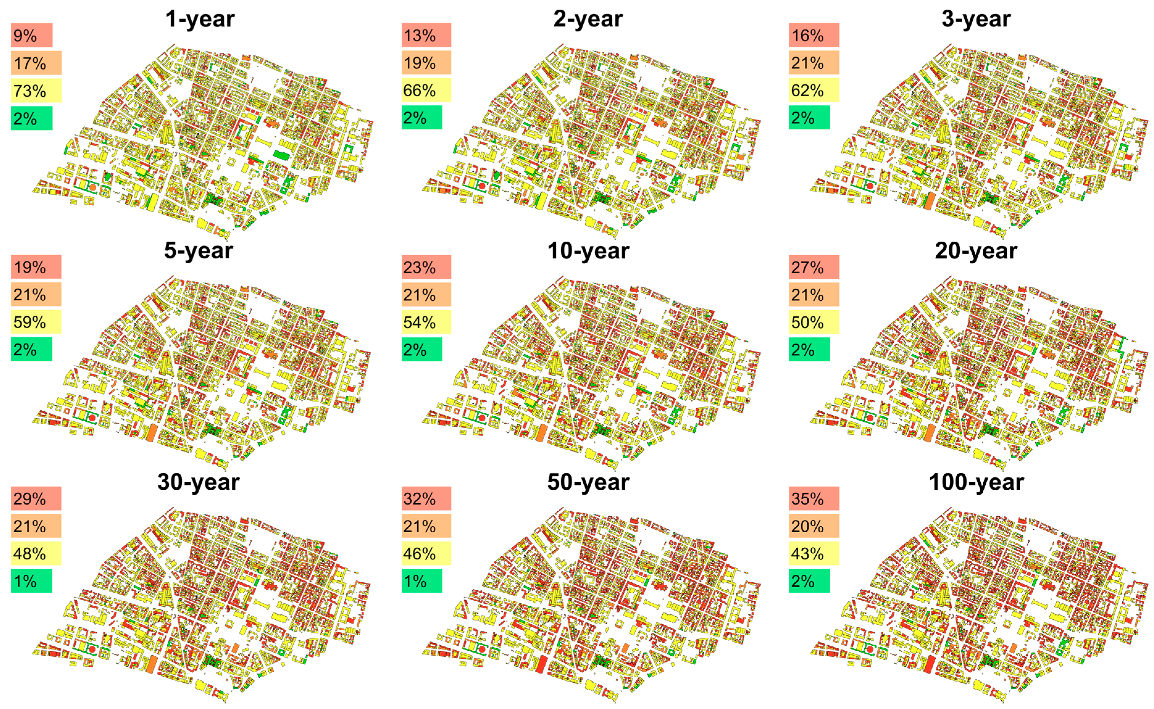
The maximum inundation modelling of the 15-min rainfall applying the data from the KOSTRA-DWD-2010R database is conducted for various return periods, providing the information of locations that are more likely to encounter severe flooding conditions in Maxvorstadt. (see Figure 4).

Table 2. Average inundation depth on streets versus return periods in Maxvorstadt.

Return Period (year)	1	2	3	5	10	20	30	50	100
Average Water Depth on Streets (cm)	4.11	5.19	5.84	6.60	7.67	8.71	9.33	10.08	11.11

shows the average inundation depth on streets versus different return periods. By applying the one-way coupling indoor water depth computation, the maximum indoor water depth for each building can be seen in Figure 5, also showing the information of the percentage of buildings facing different levels of indoor flooding.

4.2. Parameter Sensitivity Analysis

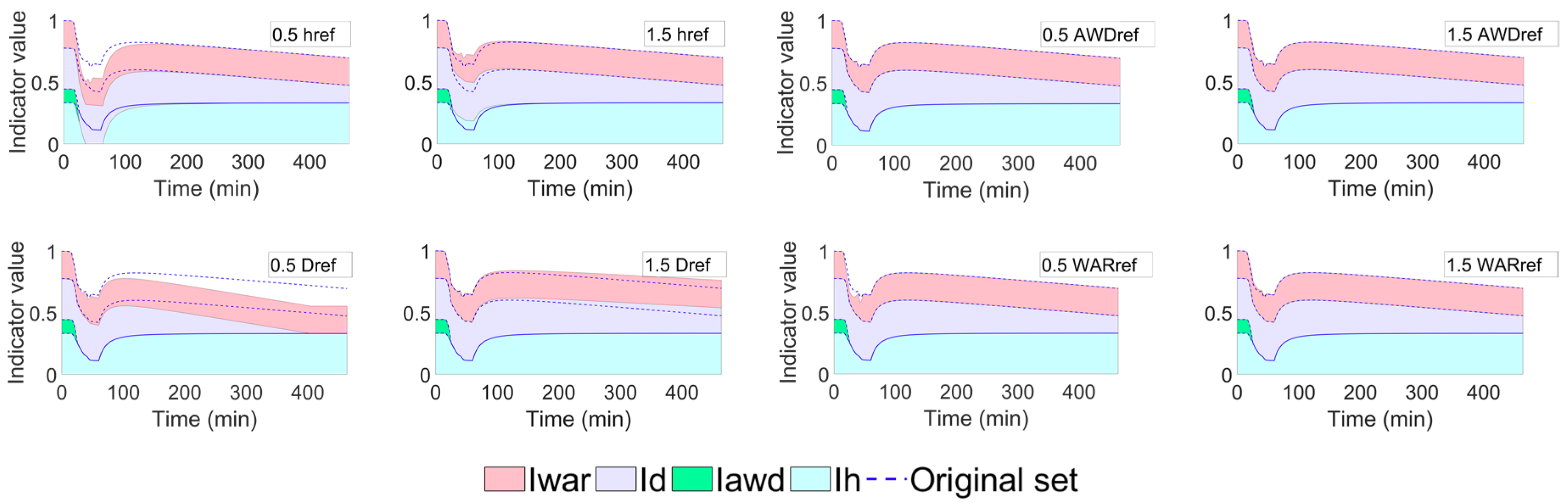
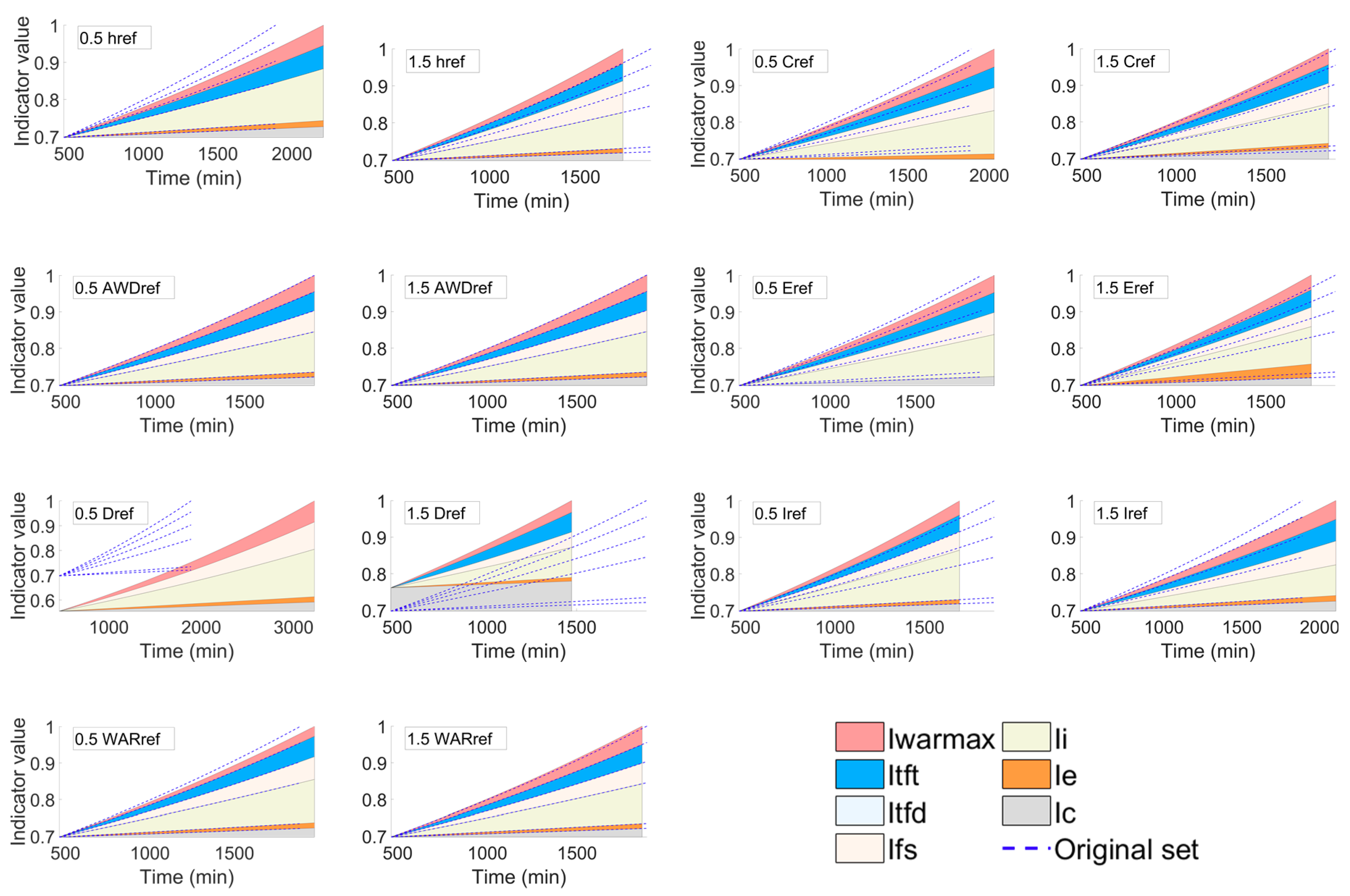
A sensitivity analysis for the reference parameters is conducted for the building which encounters the most severe indoor inundation caused by a 100-year flooding in district Königsplatz. The alteration of each indicator by changing its corresponding reference parameter is examined by comparing the case of adding and subtracting 50% from the original values of the reference parameter. The differences can be detected by comparing the case applying the original set of reference parameters (shown in blue dashed lines) and the upper edges of the areas. The results of the sensitivity analysis in the event (see Figure 6) and recovery phase (see Figure 7) are shown below.

4.3. Flood Resilience Index

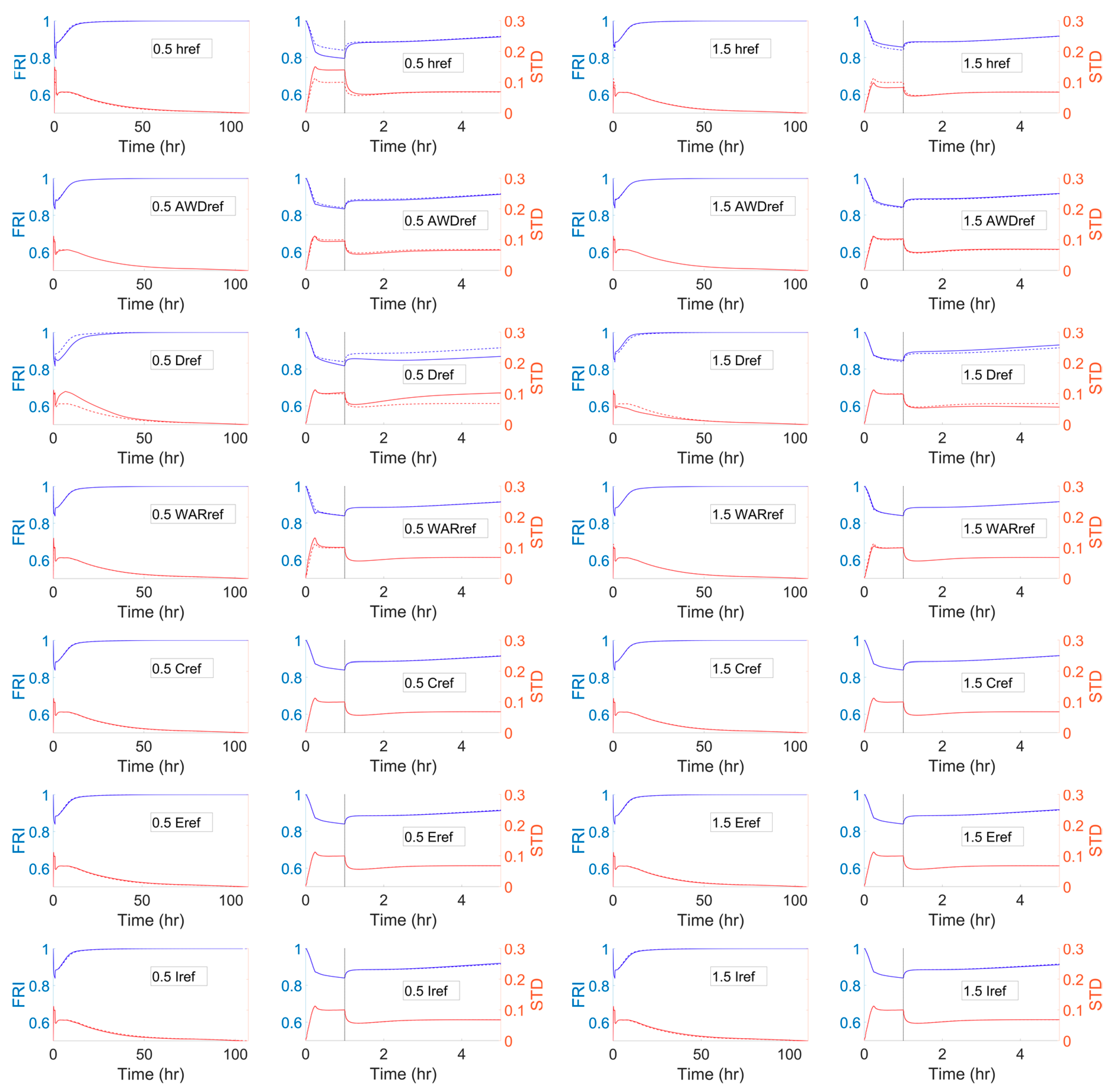
Figure 8 shows the mean FRI curves as an aggregated result for every household in Maxvorstadt according to different reference parameters (either by adding or subtracting 50% from their original values) considered in the sensitivity analysis. In addition, the standard deviation curves are provided to illustrate the level of dispersion of the FRI at each timestep.

5. Discussion

5.1. Flood Inundation Modelling

According to the results of the maximum inundation modelling (see Figure 4), it can be shown that the scenarios with higher return period as well as rainfall intensity return larger inundation areas and higher water depths. The average water depth on streets also shows an increasing trend as the return period increases (see Table 2), which corresponds to the shape of the considered 15 min rainfall intensity–frequency curve in Figure 1d. In the maximum inundation maps, there are several spots showing a small area of higher water depths. The reason is that these are areas enclosed by buildings or tunnels, which have a lower elevation than the surroundings. The surface runoff modelling applying the P-DWave model only includes the overland surface routing of rainwater. Hence, in this case, it is not possible to model the underground drainage of water accumulated at the low-laying areas. According to the maximum indoor water depth results (see Figure 5), the percentage of buildings which face a more severe indoor flooding rises as the return period increases.

5.2. Parameter Sensitivity Analysis

According to the results of parameter sensitivity analysis, different reference parameters have an effect on the corresponding FRI indicator and total FRI. In the event phase (see Figure 6), the higher the four physical reference parameters are, the higher the indicators and FRI values will be. However, the sensitiveness of changing different reference parameters differs according to the assigned weighting factors and the original values of the reference parameters. Not surprisingly, reference parameters of water depth and flooding duration, which are assigned with the greatest weighting factors, have the highest impact. The water depth reference parameter controls the water depth indicator when the building is facing an indoor flooding. As shown in Figure 6, the sensitiveness of altering such a parameter is obvious within the timeframe from 0 to 100 min, in which the building is encountering the peak water depth. By increasing this reference parameter, the water depth indicator shows a 0.1 increment at the lowest point of the indicator curve. In contrast, by decreasing this reference parameter, the water depth indicator decreases and drops to zero during the peak water depth. The sensitiveness of altering the reference parameter of flooding duration is evident at the tail end of the event phase. Like the water depth indicator, the flooding duration indicator rises when the reference parameter increases and falls down to zero at the timestep at 400 min when the reference parameter decreases. Note that changing the reference parameter of flooding duration will lead to different endpoints of the FRI in the event phase, which makes different starting points for the recovery phase. The alteration of the water accumulation rate indicator only appears at the front end of the event phase, which corresponds to the rising limb of the indoor hydrograph. The altering of the water accumulation indicator is more evident when the reference parameter decreases. However, when the indoor water is receding, the water accumulation rate becomes ineffective, and thus changing this reference parameter does not affect the water accumulation rate indicator. Finally, the reference parameter of accumulated water depth in this study is set as an extreme case (3 m) to show that by either increasing or decreasing it by 50%, the indicator will fall down to zero. The difference between these two cases is only at which timestep the indicator drops to zero. According to Figure 6, the difference between increasing and decreasing the reference parameter of accumulated water depth is not significant in this case study.

The seven indicators included in the recovery phase constitute the recovery factor which is responsible for the system to return to the original state (FRI = 1). Similar to the indicators in the event phase, the effect of reference parameters in the recovery phase depends on the assigned weighting factors and the original values of the reference parameters (see Figure 7). All indicators, with exception for the total flooding depth and income indicators, increase as their reference parameters increase. Below is a short description of the impact of each reference parameter/indicator on the recovery phase:

• Flood severity indicator—when its reference parameter decreases, the maximum water depth in the event phase becomes greater than its reference parameter, and thus the indicator is no longer contributive to the recovery factor and does not appear in the sensitivity analysis graph in the recovery phase. In this case, the system requires a longer recovery time (approximately 300 min longer) with the smaller recovery factor. On the contrary, when the reference parameter of flood severity increases, the indicator contribution to the recovery factor increases and the recovery of system is faster (200 min).
• Total flooding depth indicator—there is no difference between increasing and decreasing the reference parameter of total flooding depth as the indicator does not appear in both graphs. The reason is that the altered reference parameter remains in any case below the total water depth during the event phase, and thus the indicator has no contribution to the recovery factor.
• Total flooding time indicator—changes in the reference parameter of total flooding time show different starting points for the FRI curve at the beginning of the recovery phase. This is due to different endpoints in the event phase, as mentioned in the previous section. In this case, there will be a higher starting point in the recovery phase according to an increased reference parameter of total flooding time, and vice versa. When the reference parameter decreases, the total flooding time in the event phase exceeds the threshold, and thus the indicator is not contributive to the recovery factor and does not appear in the sensitivity analysis graph for the recovery phase. In contrast, when the reference parameter increases, not only the starting point of the recovery phase raises, but the system is able to bounce back to the original state of performance approximately 500 min faster.
• Maximum water accumulation rate indicator and households with children indicator—due to the low weighting factors assigned to both indicators, the differences between increasing or decreasing their reference parameters is relatively small. However, it can be seen that the degree of changing is larger when their reference parameters are decreased.
• Elderly population indicator—this indicator has a slightly higher impact than the two previous indicators. This is due to a larger weighting factor assigned for it. In addition, the effect of the indicator is larger when its reference parameter is increased.
• Income indicator—decreasing/increasing its reference parameter increases/decreases the indicator impact on the recovery factor. The reference parameter of income could be considered as the threshold that defines whether the income amount reaches the maximum recovery strength, at which the income indicator equals to e¹. As a result, if the reference parameter decreases, the threshold decreases, and the household will either reach the maximum recovery strength or have a larger income indicator.

The sensitivity analysis of the reference parameters provides detailed information of the FRI composition, which is a powerful tool for decision makers to decide which aspect requires instant improvement through visual comparison among indicators. The results also allow a better understanding on how external influencing factors affect the FRI. For instance, when a house is equipped with water-proof furniture, the reference parameter of water depth should raise, standing for a higher resilience to flooding depth (i.e., higher FRI).

5.3. Flood Resilience Index

According to the results of the FRI simulation (see Figure 8), the mean FRI curve drops together with an increment of the standard deviation curve at the beginning. Within the one-hour simulation duration, buildings within Maxvorstadt experience indoor flooding, and thus the mean FRI decreases in the event phase. The indoor flooding hydrograph from every building differs quite significantly. Hence, the standard deviation curve climbs, illustrating a higher level of dispersion of the FRI values. At the timestep of 1 h, the outdoor water depth is set to recede to zero (see assumptions in Section 3.3.) and the indoor water depth of each building faces a significant drop according to the one-way coupling computation, leading to a sudden increase of the mean FRI curve and a sharp drop of the standard deviation curve. Note that the recovery phase does not start at the timestep of 1 h. It starts at the timestep when the indoor water depth recedes to zero, so it differs for each building (see Figure 2). After the timestep at 1 h, the mean FRI curve climbs following the recession of indoor water depth, and gradually returns to one during the recovery phase. The standard deviation curve then returns back to zero along with the increment of the FRI values, reaching one for every building. The impact of each reference parameter on the FRI is now shortly summarized:

• Increasing/decreasing the reference parameter of water depth (event phase) and flood severity (recovery phase) increases/decreases the mean FRI curve along with a decreasing/increasing standard deviation curve.
• The altered reference parameter of accumulated water depth (event phase) and total flooding depth (recovery phase) slightly changes the mean FRI and standard deviation curve but only at the beginning of the simulation, at which the accumulated water depth does not exceed the reference parameter in the event phase.
• The altered reference parameter of flooding duration (event phase) and total flooding time (recovery phase) makes the most significant changes on the mean FRI and standard deviation curve among all considered reference parameters.
• The changes on the mean FRI and standard deviation curve due to the altered reference parameter of water accumulation rate (event phase) and maximum water accumulation rate (recovery phase) appear within the timestep at 1 h, which lies at the rising limb of all indoor hydrographs for every building. Aside from this, the effect of changing such a reference parameter is not significant.
• The altered reference parameters for the social and economic indicators can only affect the recovery phase, in which these indicators are taken into account. They are highly sensitive to the assigned weighting factors and the original set of reference parameters.
• Regarding the social and economic indicators, the altered reference parameter of income has the greatest impact on the mean FRI and standard deviation curve, while that of households with children has the least.

The summary table (see

Table 3. Summary table for the FRI simulation considering different multiplication factors of the reference parameters.

Ref. 1	Original Value	Multiplication Factor	FRI Duration 2 (h)	Lowest Mean FRI
href	0.5 m	0.5	110.4	0.79
		1.5	106.2	0.85
AWDref	3 m	0.5	107.2	0.83
		1.5	107.2	0.84
Dref	800 min	0.5	107.2	0.81
		1.5	107.2	0.84
WARref	5 cm/min	0.5	107.4	0.83
		1.5	107.1	0.83
Cref	20 %	0.5	107.7	0.83
		1.5	105.9	0.83
Eref	12 %	0.5	109.8	0.83
		1.5	106.3	0.83
Iref	80,000 €	0.5	103.8	0.83
		1.5	110.6	0.83
Original	-	1	107.2	0.83

¹ Reference parameter. ² Total duration including the event and recovery phase.

) provides information of the FRI duration (time lasting from the system being hit by flooding to a full recovery, including the event and recovery phase) and the minimum value of the mean FRI considering the effect of the altered reference parameters of each indicator. The alteration of the reference parameter of income has the highest impact considering the FRI duration, which is a 7.2 h difference comparing increasing and decreasing the reference parameter by 50%. The minimum value of the mean FRI is caused by the physical impacts from flooding and thus lies within the event phase, hence the altered reference parameters of the households with children, elderly population, and income indicators, which are only considered in the recovery phase and cannot have an effect on it. Among the four physical indicators, the alteration of the reference parameter of water depth has the largest effectiveness on the minimum mean FRI.

The aggregated FRI results provide the information of the flood resilience level within the study area (regarding it as a whole system). Based on this information, it is possible to verify whether: (a) The severity of the flooding impact hits the system and induces a significant drop of the FRI value, or (b) the system is undergoing a slow or a fast recovering process. Furthermore, the dispersiveness of the FRI curves also provides the information of how homogenously the urban components react to a certain event. If the standard deviation value is high, it means that the urban components react differently and some districts will need more assistance during low FRI periods than their neighboring zones, which have a higher FRI value.

6. Conclusions

In this paper, we developed an indicator-based flood resilience quantification method by introducing the time-varying Flood Resilience Index (FRI). The FRI is able to quantify the flood resilience level for households within an urban area, divided into event and recovery phases. Therefore, the new FRI embodies the definition of flood resilience as the capacity to withstand adverse effects following flooding events and the ability to quickly recover to the original system performance before the event. During the flooding event, the FRI is estimated based on physical indicators, namely the water depth, accumulated water depth, flooding duration, and water accumulation rate. During the recovery phase, the FRI is estimated based on social indicators, i.e., the percentage of households with children and that of elderly population, as well as an economic indicator, i.e., annual household income.

The sensitivity analysis of the parameters (and indicators) provided a useful tool to understand better how external influencing factors affect the FRI. The aggregated FRI results allow the identification of fragilities in the urban household as part of a system. It is easy to identify which households have a slow-recovering process or which are being hit severely by the event. Furthermore, the dispersiveness of the FRI curves also provides the information of how homogenously the urban components of the system react to a certain event.

The novel time-varying FRI therefore provides a novel insight into the indicator-based quantification method of flood resilience level for households in an urban area. The time-dependent characteristic of the proposed method contributes to advancing the research field by enabling a quantifiable characterization and visualization of how a system responds during and after a flooding event. Therefore, the introduced FRI could become a valuable tool for urban planning and public communication, and promote a better flood risk management plan. Future work will see the inclusion of the sewer network and possible extension of the urban area of Maxvorstadt, which is considered at the moment isolated from other boroughs in Munich City.

References

- Barroca, B.; Bernardara, P.; Mouchel, J.M.; Hubert, G. Indicators for identification of urban flooding vulnerability. Nat. Hazards Earth Syst. Sci. 2006, 6, 553–561. [Google Scholar] [CrossRef]
- Campbell, J.; Douglas, I.; Mclean, L.; Mcdonnell, Y.; Alam, K.; Maghenda, M. Unjust waters: Climate change, flooding and the urban poor in Africa. Environ. Urban. 2008, 20, 187–205. [Google Scholar]
- Few, R. Flooding, vulnerability and coping strategies: Local responses to a global threat. Prog. Dev. Stud. 2003, 3, 43–58. [Google Scholar] [CrossRef]
- Adelekan, I.O. Vulnerability of poor urban coastal communities to flooding in Lagos, Nigeria. Environ. Urban. 2010, 22, 433–450. [Google Scholar] [CrossRef]
- Huong, H.; Pathirana, A. Urbanization and climate change impacts on future urban flooding in Can Tho city, Vietnam. Hydrol. Earth Syst. Sci. 2013, 17, 379–394. [Google Scholar] [CrossRef]
- Hallegatte, S. Strategies to adapt to an uncertain climate change. Glob. Environ. Chang. 2009, 19, 240–247. [Google Scholar] [CrossRef]
- Jones, H.P.; Hole, D.G.; Zavaleta, E.S. Harnessing nature to help people adapt to climate change. Nat. Clim. Chang. 2012, 2, 504–509. [Google Scholar] [CrossRef]
- Leandro, J. Title of Special Issue: Towards more Flood Resilient Cities. Urban Water J. 2015, 12, 1–2. [Google Scholar] [CrossRef]
- Robadue, D., Jr. Understanding resistance to resilience in coastal hazards and climate adaptation: Three approaches to visualizing structural and process obstacles, opportunities and adaptation responses. In Proceedings of the 52nd Hawaii International Conference on System Sciences, Maui, HI, USA, 8–11 January 2019. [Google Scholar]
- Messner, F.; Penning-Rowsell, E.; Green, C.; Meyer, V.; Tunstall, S.; van der Veen, A. Evaluating Flood Damages: Guidance and Recommendations on Principles and Methods; FLOODsite: Wallingford, UK, 2007. [Google Scholar]
- Schelfaut, K.; Pannemans, B.; van der Craats, I.; Krywkow, J.; Mysiak, J.; Cools, J. Bringing flood resilience into practice: The FREEMAN project. Environ. Sci. Policy 2011, 14, 825–833. [Google Scholar] [CrossRef]
- Jones, L. Resilience isn’t the same for all: Comparing subjective and objective approaches to resilience measurement. Wiley Interdiscip. Rev. Clim. Chang. 2019, 10, e552. [Google Scholar] [CrossRef]
- Allen, T.R.; Crawford, T.; Montz, B.; Whitehead, J.; Lovelace, S.; Hanks, A.D.; Christensen, A.R.; Kearney, G.D. Linking Water Infrastructure, Public Health, and Sea Level Rise: Integrated Assessment of Flood Resilience in Coastal Cities. Public Work. Manag. Policy 2019, 24, 110–139. [Google Scholar] [CrossRef]
- Moghadas, M.; Asadzadeh, A.; Vafeidis, A.; Fekete, A.; Kötter, T. A multi-criteria approach for assessing urban flood resilience in Tehran, Iran. Int. J. Disaster Risk Reduct. 2019, 35, 101069. [Google Scholar] [CrossRef]
- Zhang, Y.; Li, W.; Sun, G.; King, J.S. Coastal wetland resilience to climate variability: A hydrologic perspective. J. Hydrol. 2019, 568, 275–284. [Google Scholar] [CrossRef]
- Karamouz, M.; Taheri, M.; Khalili, P.; Chen, X. Building Infrastructure Resilience in Coastal Flood Risk Management. J. Water Resour. Plan. Manag. 2019, 145, 4019004. [Google Scholar] [CrossRef]
- Murdock, H.; de Bruijn, K.; Gersonius, B. Assessment of Critical Infrastructure Resilience to Flooding Using a Response Curve Approach. Sustainability 2018, 10, 3470. [Google Scholar] [CrossRef]
- Walsh, B.; Hallegatte, S. Measuring Natural Risks in the Philippines: Socioeconomic Resilience and Wellbeing Losses; World Bank Group: Washington, DC, USA, 2019. [Google Scholar]
- Driessen, P.; Hegger, D.; Kundzewicz, Z.; van Rijswick, H.; Crabbé, A.; Larrue, C.; Matczak, P.; Pettersson, M.; Priest, S.; Suykens, C.; et al. Governance Strategies for Improving Flood Resilience in the Face of Climate Change. Water 2018, 10, 1595. [Google Scholar] [CrossRef]
- Hammond, M.J.; Chen, A.S.; Djordjević, S.; Butler, D.; Mark, O. Urban flood impact assessment: A state-of-the-art review. Urban Water J. 2015, 12, 14–29. [Google Scholar] [CrossRef]
- Holling, C.S. Resilience and Stability of Ecological Systems. Annu. Rev. Ecol. Syst. 1973, 4, 1–23. [Google Scholar] [CrossRef]
- de Bruijn, K.M. Resilience and flood risk management. Water Policy 2004, 6, 53–66. [Google Scholar] [CrossRef]
- Tourbier, J. A Methodology to Define Flood Resilience. In Proceedings of the EGU General Assembly, Vienna, Austria, 22–27 April 2012. [Google Scholar]
- United Nations Office for Disaster Risk Reduction. Terminology on Disaster Risk Reduction. Available online: https://www.unisdr.org/we/inform/terminology#letter-r (accessed on 15 December 2018).
- Mugume, S.; Gomez, D.; Butler, D. Quantifying the resilience of urban drainage systems using a hydraulic performance assessment approach. In Proceedings of the 13th International Conference on Urban Drainage, Sarawak, Malaysia, 7–12 September 2014. [Google Scholar]
- Perfrement, T.; Lloyd, T. Identifying and Visaulising Resilience to Flooding via a Composite Flooding Disaster Resilience Index. In Proceedings of the 56th Floodplain Management Australia National Conference, Nowra, Australia, 17–20 May 2016. [Google Scholar]
- Keating, A.; Campbell, K.; Szoenyi, M.; McQuistan, C.; Nash, D.; Burer, M. Development and testing of a community flood resilience measurement tool. Nat. Hazards Earth Syst. Sci. 2017, 17, 77–101. [Google Scholar] [CrossRef]
- Bizzotto, M. Resilient Cities Report 2018. In Proceedings of the 9th Global Forum on Urban Resilience and Adaptation, Bonn, Germany, 26–28 April 2018. [Google Scholar]
- The Rockefeller Foundation and ARUP. City Resilience Index; ARUP: London, UK, 2014. [Google Scholar]
- Fischer, K.; Hiermaier, S.; Riedel, W.; Häring, I. Morphology Dependent Assessment of Resilience for Urban Areas. Sustainability 2018, 10, 1800. [Google Scholar] [CrossRef]
- Winderl, T. Disaster Resilience Measurements: Stocktaking of Ongoing Efforts in Developing Systems for Measuring Resilience; United Nations Development Programme: New York, NY, USA, 2014. [Google Scholar]
- de Bruijn, K.M. Resilience indicators for flood risk management systems of lowland rivers. Int. J. River Basin Manag. 2004, 2, 199–210. [Google Scholar] [CrossRef]
- Gourbesville, P.; Batica, J. Flood Resilience Index—Methodology and Application. In Proceedings of the 11th International Conference on Hydroinformatics, New York, NY, USA, 17–21 August 2014. [Google Scholar]
- Lee, E.H.; Kim, J.H. Development of Resilience Index Based on Flooding Damage in Urban Areas. Water 2017, 9, 428. [Google Scholar] [CrossRef]
- Bertilsson, L.; Wiklund, K.; de Moura Tebaldi, I.; Rezende, O.M.; Veról, A.P.; Miguez, M.G. Urban flood resilience—A multi-criteria index to integrate flood resilience into urban planning. J. Hydrol. 2018, in press. [Google Scholar] [CrossRef]
- Landeshauptstadt München. Statistisches Taschenbuch 2018—München und seine Stadtbezirke; Landeshauptstadt München: Munich, Germany, 2018.
- Landeshauptstadt Munchen. Munich Facts and Figures 2018; Landeshauptstadt Munchen: Munich, Germany, 2018.
- Junghänel, T.; Ertel, H.; Deutschländer, T. Bericht zur Revision der koordinierten Starkregenregionalisierung und -auswertung des Deutschen Wetterdienstes in der Version 2010; Deutscher Wetterdienst: Offenbach am Main, Germany, 2017.
- Young, G. From Chemical Exposure and Mold to Mosquitos, Problems Don’t Stop When the Rain Does. Available online: https://today.ttu.edu/posts/2015/06/flooding-long-term-impact-health-environment (accessed on 20 November 2018).
- Unterberger, C. How Flood Damages to Public Infrastructure Affect Municipal Budget Indicators. Econ. Disasters Clim. Chang. 2018, 2, 5–20. [Google Scholar] [CrossRef]
- Ten Brinke, W.; Knoop, J.; Muilwijk, H.; Ligtvoet, W. Social disruption by flooding, a European perspective. Int. J. Disaster Risk Reduct. 2017, 21, 312–322. [Google Scholar] [CrossRef]
- Milojevic, A.; Armstrong, B.; Wilkinson, P. Mental health impacts of flooding: A controlled interrupted time series analysis of prescribing data in England. J. Epidemiol. Community Heal. 2017, 71, 970–973. [Google Scholar] [CrossRef]
- Rufat, S.; Tate, E.; Burton, C.G.; Maroof, A.S. Social vulnerability to floods: Review of case studies and implications for measurement. Int. J. Disaster Risk Reduct. 2015, 14, 470–486. [Google Scholar] [CrossRef]
- Teo, M.; Goonetilleke, A.; Ziyath, A.M. An integrated framework for assessing community resilience in disaster management. In Proceedings of the 9th Annual International Conference of the International Institute for Infrastructure Renewal and Reconstruction, Risk-informed Disaster Management: Planning for Response, Recovery and Resilience, Brisbane, Australia, 7–10 July 2013. [Google Scholar]
- Saja, A.; Goonetilleke, A.; Teo, M.; Ziyath, A. A critical review of social resilience assessment frameworks in disaster management. Int. J. Disaster Risk Reduct. 2019, 35, 101096. [Google Scholar] [CrossRef]
- Leandro, J.; Chen, A.; Schumann, A. A 2D parallel diffusive wave model for floodplain inundation with variable time step (P-DWave). J. Hydrol. 2014, 517, 250–259. [Google Scholar] [CrossRef]
Figure 1.
(a) Location of the nine districts and buildings within Maxvorstadt; and (b) demographic structure with age distribution of Maxvorstadt. The size of the age pie chart is proportional to the population amount. (c) Land use map of Maxvorstadt; and (d) Rainfall Intensity Duration Frequency curve of Maxvorstadt. Data retrieved from KOSTRA-DWD-2010R database (Grid no. 92049) containing information from 1951 to 2010. This paper applies the 15 min duration rainfall events for various return periods.
Figure 2.
Illustration of the Flood Resilience Index (FRI) structure. t* stands for the timestep when the indoor water depth returns to zero, which separates the event and recovery phases.
Figure 3.
One-way coupling computation of the flow dynamic of water coming into the building. The upper portion of the flow, in which the water level outside the building is higher than the water depth inside the building, is marked as 1, and the lower portion, in which the water level outside the building is equal to the water depth inside the building, is marked as 2. h_outside and h_inside stand for the water depth outside and inside the building, respectively. When the indoor water depth is higher than that of the outdoor surroundings, the computation remains the same, whereas the discharge becomes negative as the flow direction faces the opposite direction.
Figure 4.
Maximum inundation map in Maxvorstadt with various return periods, applying rainfall data from the KOSTRA-DWD-2010R database. Luisen Street, located at the center of Maxvorstadt, faces the most extreme flooding condition with the range crossing over two blocks and maximum water depth over 50 cm in the case of a 100-year flooding event.
Figure 5.
Maximum indoor water depth modelling given flooding events with various return periods by applying the one-way coupling computation. The indoor water depth in buildings with color green: 0 cm, yellow: 0–5 cm, orange: 5–10 cm, and red: above 10 cm. Percentage stands for the amount of building in each level of indoor flooding.
Figure 6.
Sensitivity analysis of the four reference parameters for each physical indicator in the event phase by comparing the case of adding and subtracting 50% from the original reference parameters. Blue dashed line stands for the case when applying the original set of reference parameters. Annotation in each graph illustrates which reference parameter is examined by either adding or subtracting 50% from its original value.
Figure 7.
Sensitivity analysis of the seven reference parameters for each physical, social, and economic indicator in the recovery phase by comparing the case of adding and subtracting 50% from the original reference parameters. Blue dashed line stands for the case when applying the original set of reference parameters. Annotation in each graph illustrates which reference parameter is examined by either adding or subtracting 50% from its original value.
Figure 8.
Mean FRI curves as aggregated results for every household in Maxvorstadt (blue lines) and standard deviation curves (red lines) showing the level of dispersion of the FRI at each timestep in face of a 100-year flooding. The simulation considers different multiplication factors of the reference parameters applied in the sensitivity analysis. Solid lines represent the considered case (either with a 50% increment or decrement of the original reference parameter) and the dashed lines correspond to the case applying the original set of reference parameters. Black dashed lines at t = 1 h in the zoom-in graphs (right-hand side) illustrate the end of the outdoor inundation modelling, for which the outdoor water depth is set to zero to enable the start of the recovery phase.