A Physically Based Empirical Localization Method for Assimilating Synthetic SWOT Observations of a Continental-Scale River: A Case Study in the Congo Basin


Abstract
:1. Introduction
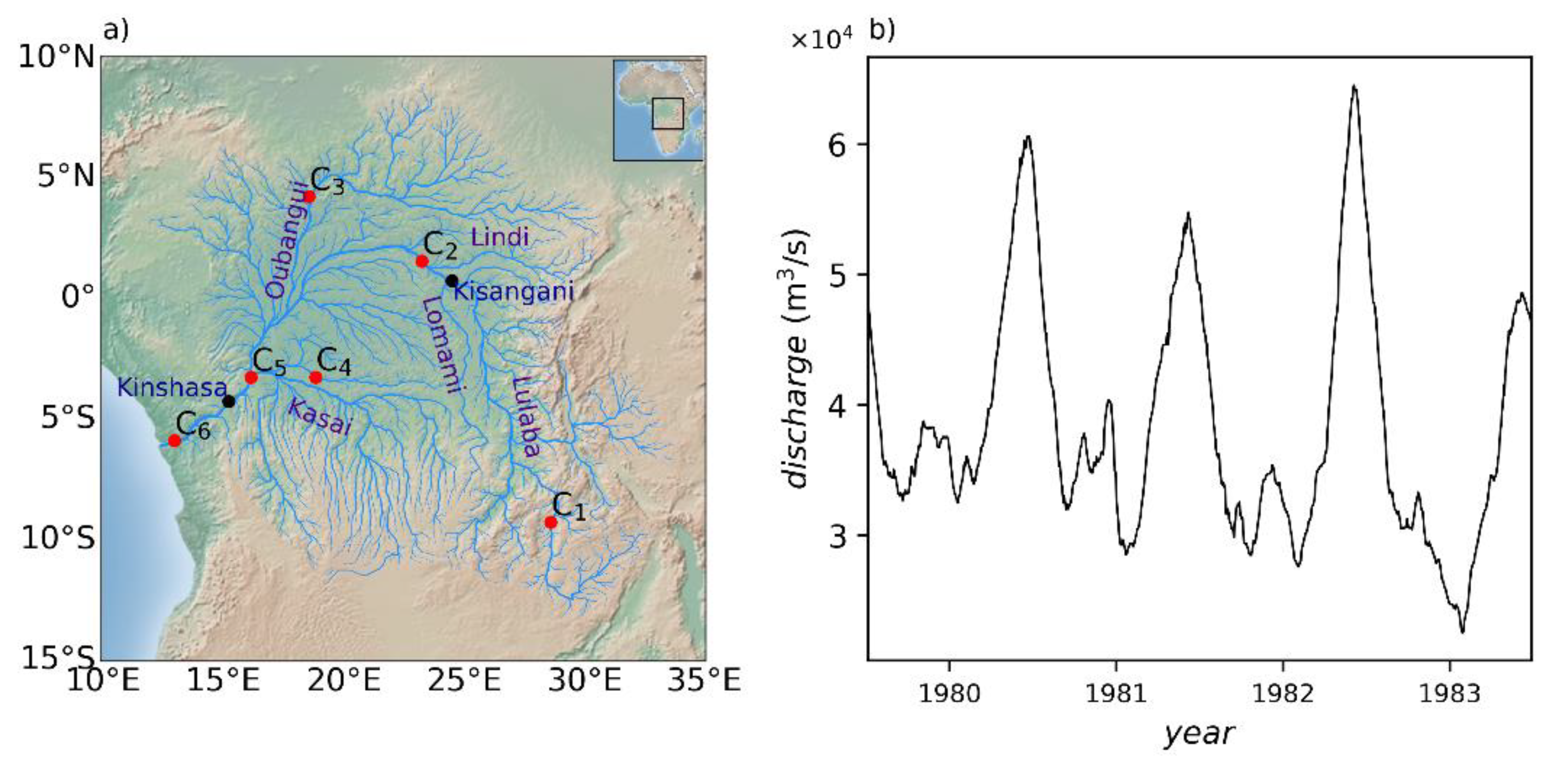
2. Study Area
3. Methodology
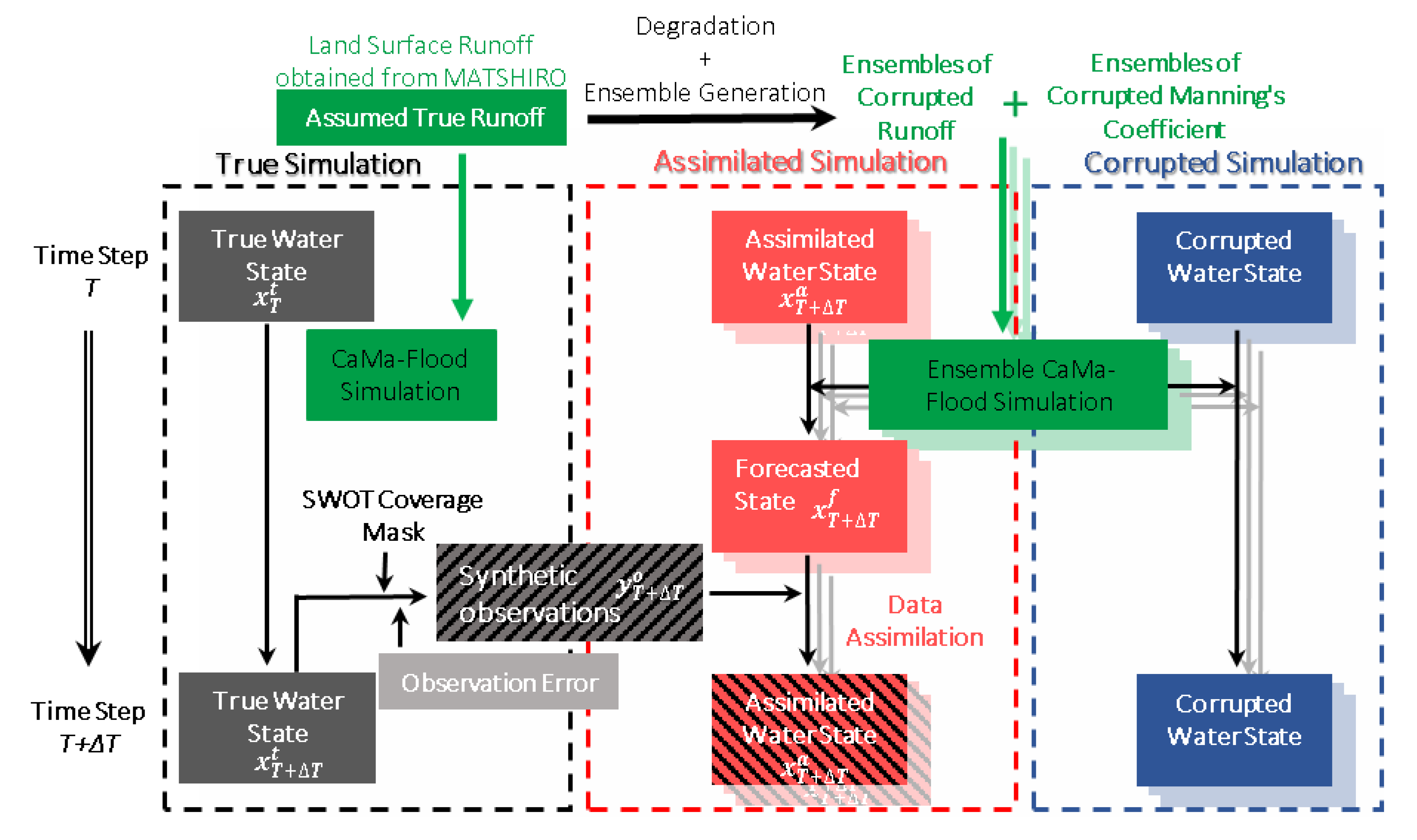
3.1. Framework of the Virtual Assimilation Experiment
3.2. Hydrodynamic Model Description and Implementation
3.3. Data Assimilation Strategy
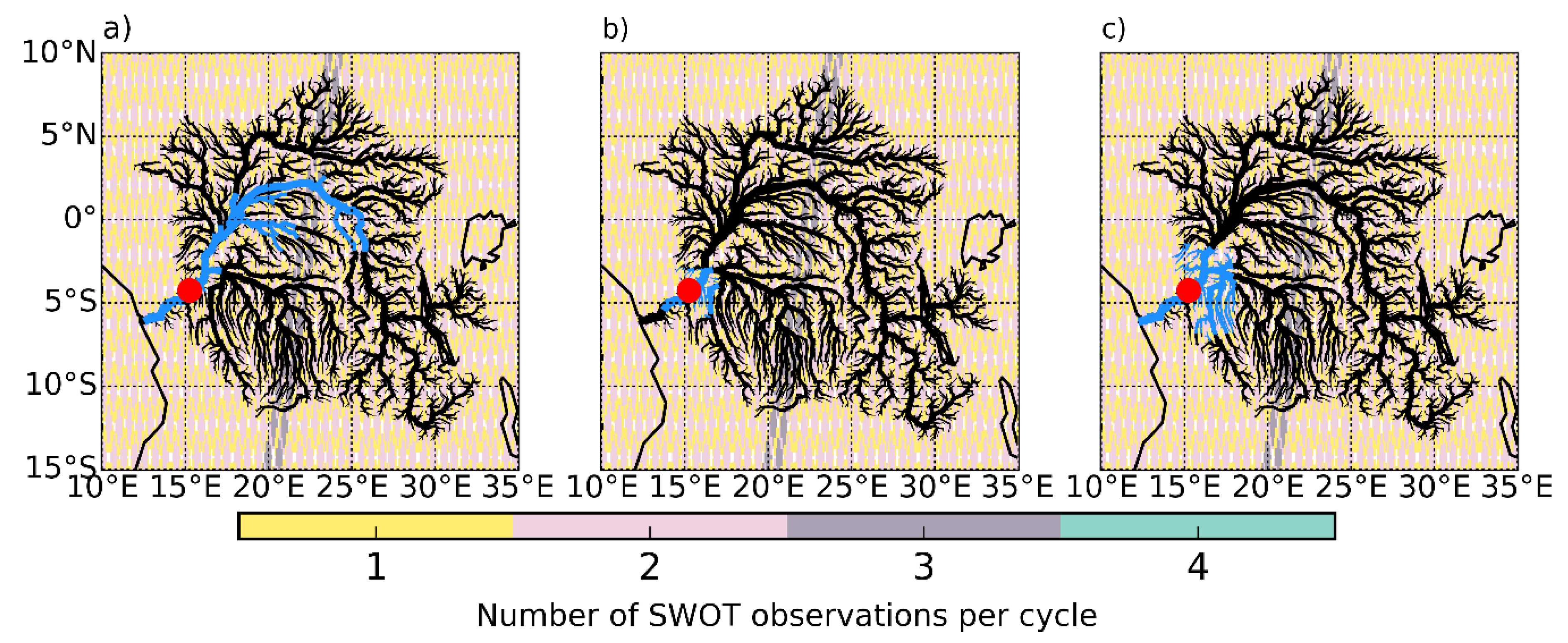
3.4. Generation of Synthetic SWOT Observations
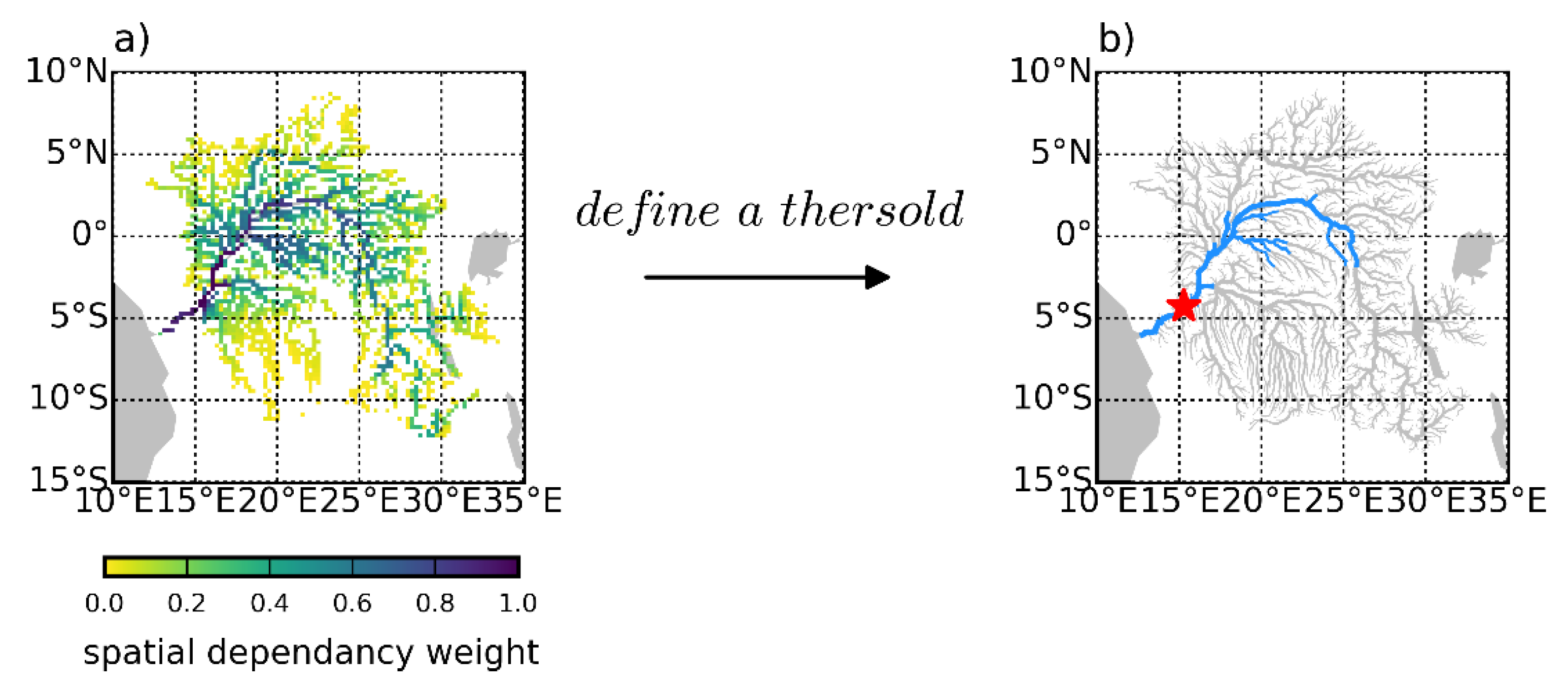
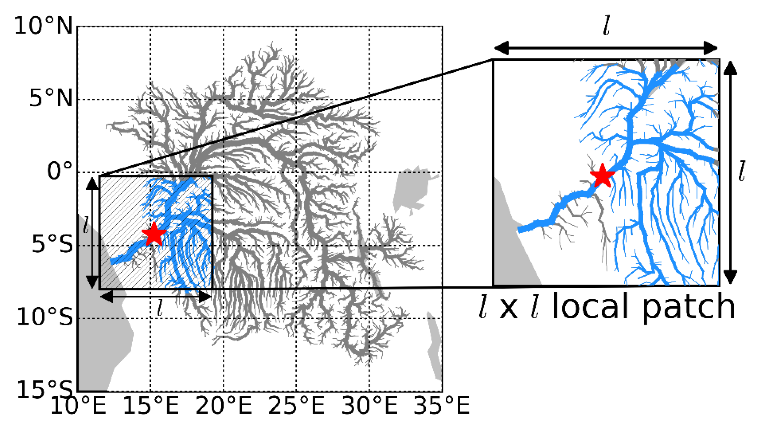
3.5. Empirical Determination of the Local Patch
4. Experimental Conditions
4.1. Empirical Local Patch Experiment
4.2. Zero Local Patch Experiment
4.3. Fixed Local Patch Experiment
4.4. Evaluation Method
5. Results and Discussion
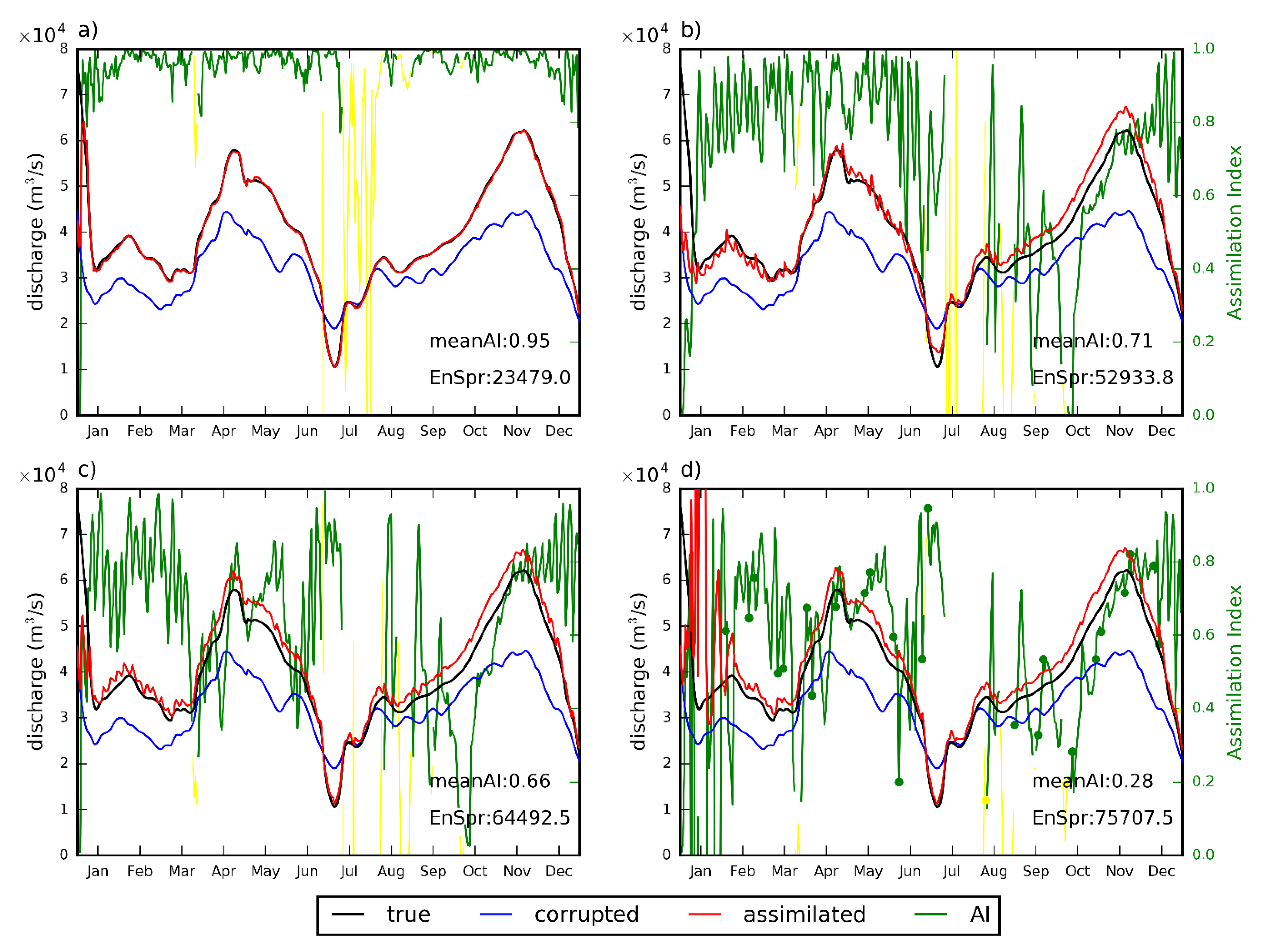
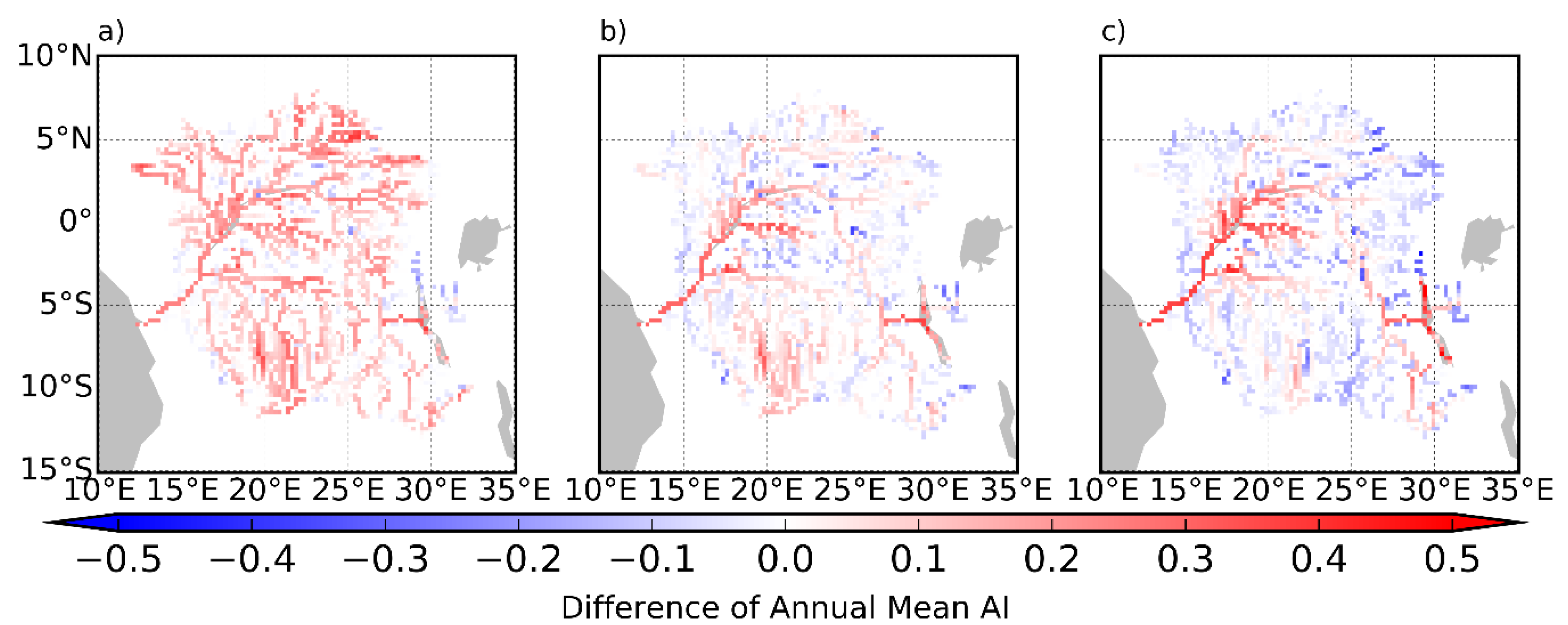
5.1. Empirical Local Patch Experiment
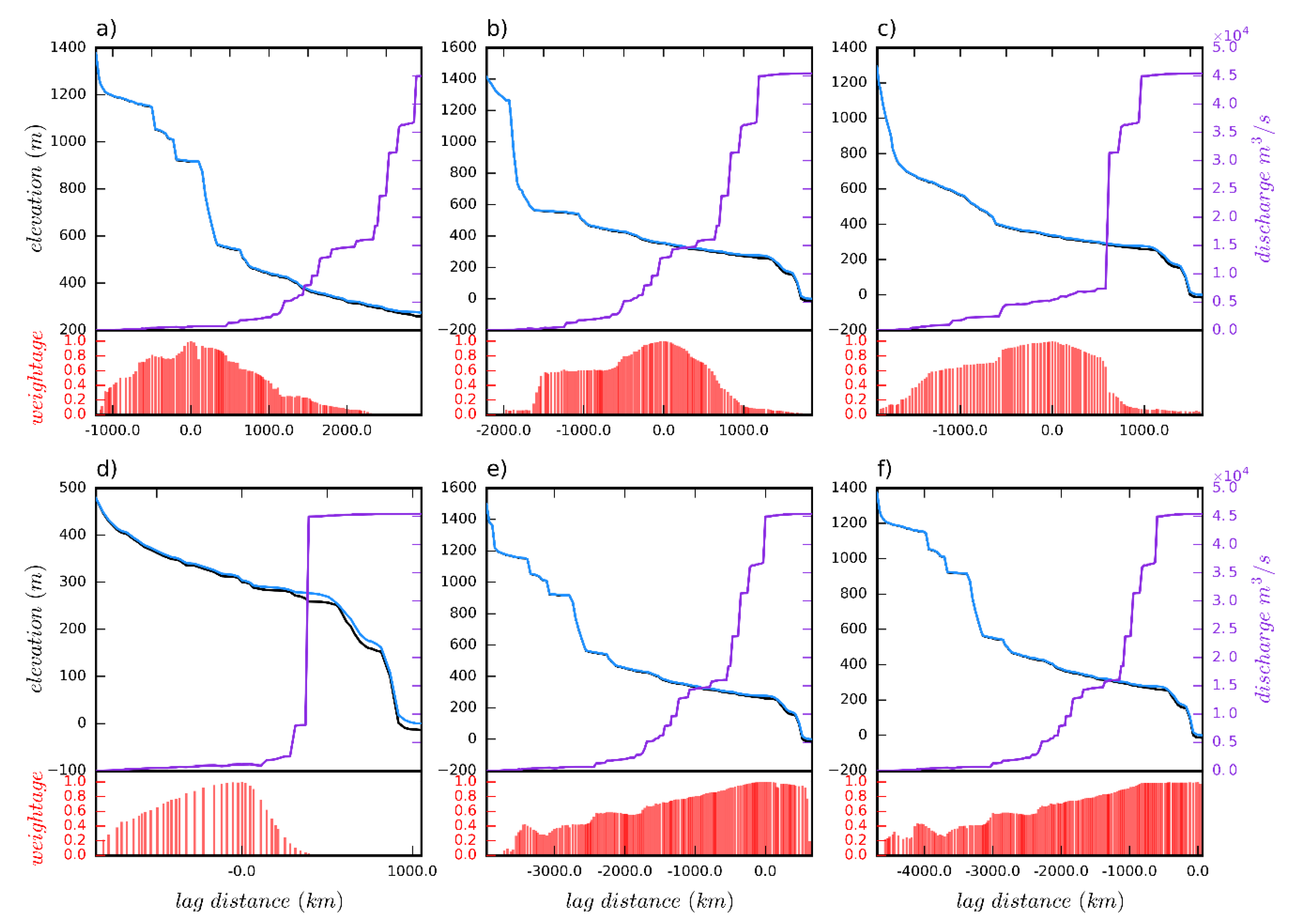
5.1.1. Empirical Local Patches
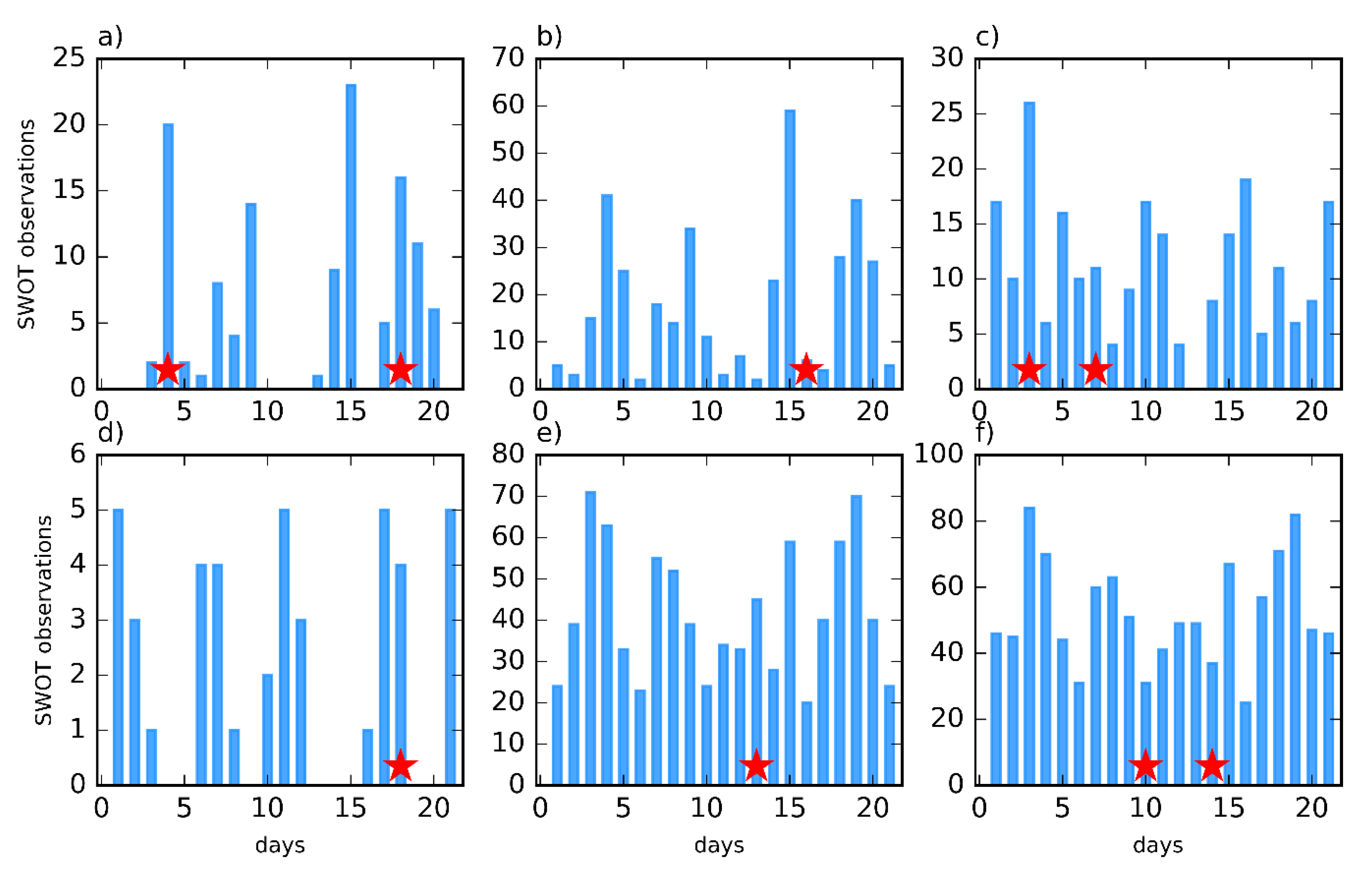
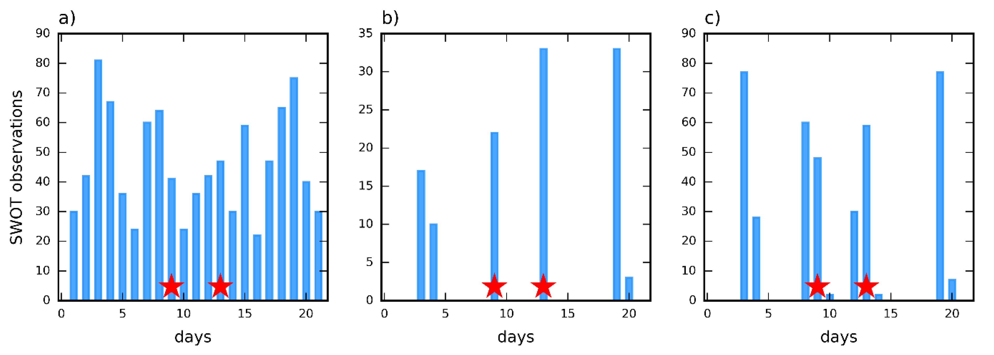
5.1.2. Observation Frequency
5.1.3. Physically Based Observation Localization
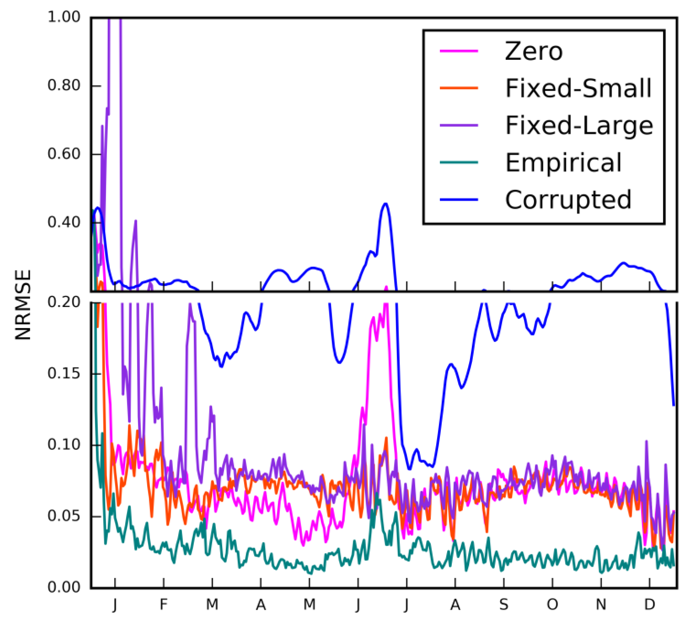
5.2. Comparison among OSSEs
5.3. Assimilation Efficiency
5.4. Computational Efficiency
6. Conclusions
Supplementary Materials
Author Contributions
Funding
Acknowledgments
Conflicts of Interest
References
- Oki, T.; Kanae, S. Global Hydrological Cycles and World Water Resources. Science 2006, 5790, 1068–1072. [Google Scholar] [CrossRef]
- Yoon, Y.; Durand, M.; Merry, C.J.; Clark, E.A.; Andreadis, K.M.; Alsdorf, D.E. Estimating River Bathymetry from Data Assimilation of Synthetic SWOT Measurements. J. Hydrol. 2012, 464, 363–375. [Google Scholar] [CrossRef]
- Alsdorf, D.E.; Rodríguez, E.; Lettenmaier, D.P. Measuring Surface Water from Space. Rev. Geophys. 2007, 45, RG2002. [Google Scholar] [CrossRef]
- Durand, M.; Rodríguez, E.; Alsdorf, D.E.; Trigg, M. Estimating River Depth from Remote Sensing Swath Interferometry Measurements of River Height, Slope, and Width. IEEE J. Sel. Top. Appl. Earth Obs. Remote Sens. 2010, 3, 20–31. [Google Scholar] [CrossRef]
- Biancamaria, S.; Durand, M.; Andreadis, K.M.; Bates, P.D.; Boone, A.; Mognard, N.M.; Rodríguez, E.; Alsdorf, D.E.; Lettenmaier, D.P.; Clark, E.A. Assimilation of Virtual Wide Swath Altimetry to Improve Arctic River Modeling. Remote Sens. Environ. 2011, 115, 373–381. [Google Scholar] [CrossRef]
- Durand, M.; Fu, L.L.; Lettenmaier, D.P.; Alsdorf, D.E.; Rodriguez, E.; Esteban-Fernandez, D. The Surface Water and Ocean Topography Mission: Observing Terrestrial Surface Water and Oceanic Submesoscale Eddies. Proc. IEEE 2010, 98, 766–779. [Google Scholar] [CrossRef]
- Lee, H.; Durand, M.; Jung, H.C.; Alsdorf, D.; Shum, C.K.; Sheng, Y. Characterization of Surface Water Storage Changes in Arctic Lakes Using Simulated SWOT Measurements. Int. J. Remote Sens. 2010, 31, 14–3931. [Google Scholar] [CrossRef]
- Reichle, R.H. Data Assimilation Methods in the Earth Sciences. Adv. Water Resour. 2008, 31, 1411–1418. [Google Scholar] [CrossRef]
- Giustarini, L.; Matgen, P.; Hostache, R.; Montanari, M.; Plaza, D.; Pauwels, V.R.N.; De Lannoy, G.J.M.; De Keyser, R.; Pfister, L.; Hoffmann, L.; et al. Assimilating SAR-Derived Water Level Data into a Hydraulic Model: A Case Study. Hydrol. Earth Syst. Sci. 2011, 15, 2349–2365. [Google Scholar] [CrossRef]
- Andreadis, K.M.; Clark, E.A.; Lettenmaier, D.P.; Alsdorf, D.E. Prospects for River Discharge and Depth Estimation through Assimilation of Swath-Altimetry into a Raster-Based Hydrodynamics Model. Geophys. Res. Lett. 2007, 34, 1–5. [Google Scholar] [CrossRef]
- Andreadis, K.M.; Schumann, G.J.P. Estimating the Impact of Satellite Observations on the Predictability of Large-Scale Hydraulic Models. Adv. Water Resour. 2014, 73, 44–54. [Google Scholar] [CrossRef]
- Durand, M.; Andreadis, K.M.; Alsdorf, D.E.; Lettenmaier, D.P.; Moller, D.; Wilson, M. Estimation of Bathymetric Depth and Slope from Data Assimilation of Swath Altimetry into a Hydrodynamic Model. Geophys. Res. Lett. 2008, 35, 1–5. [Google Scholar] [CrossRef]
- Pedinotti, V.; Boone, A.; Ricci, S.; Biancamaria, S.; Mognard, N. Assimilation of Satellite Data to Optimize Large-Scale Hydrological Model Parameters: A Case Study for the SWOT Mission. Hydrol. Earth Syst. Sci. 2014, 18, 4485–4507. [Google Scholar] [CrossRef]
- Hunt, B.R.; Kostelich, E.J.; Szunyogh, I. Efficient Data Assimilation for Spatiotemporal Chaos: A Local Ensemble Transform Kalman Filter. Phys. D Nonlinear Phenom. 2007, 230, 112–126. [Google Scholar] [CrossRef]
- Miyoshi, T.; Yamane, S.; Enomoto, T. Localizing the Error Covariance by Physical Distances within a Local Ensemble Transform Kalman Filter (LETKF). Sola 2007, 3, 89–92. [Google Scholar] [CrossRef]
- Houtekamer, P.L.; Mitchell, H.L.; Houtekamer, P.L.; Mitchell, H.L. A Sequential Ensemble Kalman Filter for Atmospheric Data Assimilation. Mon. Weather Rev. 2001, 129, 123–137. [Google Scholar] [CrossRef]
- Anderson, J.L. Exploring the Need for Localization in Ensemble Data Assimilation Using a Hierarchical Ensemble Filter. Phys. D Nonlinear Phenom. 2007, 230, 99–111. [Google Scholar] [CrossRef]
- Miyoshi, T.; Yamane, S. Local Ensemble Transform Kalman Filtering with an AGCM at a T159/L48 Resolution. Mon. Weather Rev. 2007, 135, 3841–3861. [Google Scholar] [CrossRef]
- Miyoshi, T. The Gaussian Approach to Adaptive Covariance Inflation and Its Implementation with the Local Ensemble Transform Kalman Filter. Mon. Weather Rev. 2011, 139, 1519–1535. [Google Scholar] [CrossRef]
- Munier, S.; Polebistki, A.; Brown, C.; Belaud, G.; Lettenmaier, D.P. SWOT Data Assimilation for Operational Reservoirmanagement on the Upper Niger River Basin S. Water Resour. Res. 2015, 51, 554–575. [Google Scholar] [CrossRef]
- Yoon, Y.; Durand, M.; Merry, C.J.; Rodriguez, E. Improving Temporal Coverage of the SWOT Mission Using Spatiotemporal Kriging. IEEE J. Sel. Top. Appl. Earth Obs. Remote Sens. 2013, 6, 1719–1729. [Google Scholar] [CrossRef]
- Yamazaki, D.; Kanae, S.; Kim, H.; Oki, T. A Physically Based Description of Floodplain Inundation Dynamics in a Global River Routing Model. Water Resour. Res. 2011, 47. [Google Scholar] [CrossRef]
- Domeneghetti, A.; Schumann, G.J.P.; Frasson, R.P.M.; Wei, R.; Pavelsky, T.M.; Castellarin, A.; Brath, A.; Durand, M.T. Characterizing Water Surface Elevation under Different Flow Conditions for the Upcoming SWOT Mission. J. Hydrol. 2018, 561, 848–861. [Google Scholar] [CrossRef]
- Revel, M.; Yamazaki, D.; Kanae, S. Estimating Global River Bathymetry by Assimilating Synthetic SWOT Measurements. Annu. J. Hydraul. Eng. JSCE 2018, 74, I_307–I_312. [Google Scholar] [CrossRef]
- SWOT Orbit. Available online: https://www.aviso.altimetry.fr/en/missions/future-missions/swot/orbit.html (accessed on 6 January 2018).
- Yamazaki, D.; Lee, H.; Alsdorf, D.E.; Dutra, E.; Kim, H.; Kanae, S.; Oki, T. Analysis of the Water Level Dynamics Simulated by a Global River Model: A Case Study in the Amazon River. Water Resour. Res. 2012, 48. [Google Scholar] [CrossRef]
- Yamazaki, D.; De Almeida, G.A.M.; Bates, P.D. Improving Computational Efficiency in Global River Models by Implementing the Local Inertial Flow Equation and a Vector-Based River Network Map. Water Resour. Res. 2013, 49, 7221–7235. [Google Scholar] [CrossRef]
- Bates, P.D.; Horritt, M.S.; Fewtrell, T.J. A Simple Inertial Formulation of the Shallow Water Equations for Efficient Two-Dimensional Flood Inundation Modelling. J. Hydrol. 2010, 387, 33–45. [Google Scholar] [CrossRef]
- Takata, K.; Emori, S.; Watanabe, T. Development of the Minimal Advanced Treatments of Surface Interaction and Runoff. Glob. Planet. Chang. 2003, 38, 209–222. [Google Scholar] [CrossRef]
- Kim, H.; Yeh, P.J.F.; Oki, T.; Kanae, S. Role of Rivers in the Seasonal Variations of Terrestrial Water Storage over Global Basins. Geophys. Res. Lett. 2009, 36, 2–6. [Google Scholar] [CrossRef]
- Evensen, G. The Ensemble Kalman Filter for Combined State and Parameter Estimation. IEEE Control Syst. 2009, 29, 83–104. [Google Scholar] [CrossRef]
- Te Chow, V. Open Channel Hydraulics; McGraw-Hill: New York, NY, USA, 1959. [Google Scholar]
- Barnes, H.H. Roughness Characteristics of Natural Channels; United States Government Printing Office: Washington, DC, USA, 1967.
- Akan, A.O. Open Channel Hydraulics; Elsevier Ltd.: Oxford, UK, 2006. [Google Scholar]
- Kalman, R.E. A New Approach to Linear Filtering and Prediction Problems. J. Basic Eng. 1960, 82, 35. [Google Scholar] [CrossRef]
- Hamill, T.M.; Whitaker, J.S.; Snyder, C. Distance-Dependent Filtering of Background Error Covariance Estimates in an Ensemble Kalman Filter. Mon. Weather Rev. 2001, 129, 2776–2790. [Google Scholar] [CrossRef]
- Ikeshima, D.; Yamazaki, D.; Shinjiro, K. Application of Data Assimilation for a Global River Model: A Virtual Experiment at the Amazon Basin. Annu. J. Hydraul. Eng. JSCE 2017, 73, I_175–I_180. [Google Scholar] [CrossRef]
- Nash, J.E.; Sutcliffe, J.V. River Flow Forecasting Through Conceptual Models Part I-a Discussion of Principles. J. Hydrol. 1970, 10, 282–290. [Google Scholar] [CrossRef]
- Anderson, J.L. Localization and Sampling Error Correction in Ensemble Kalman Filter Data Assimilation. Mon. Weather Rev. 2012, 140, 2359–2371. [Google Scholar] [CrossRef]
- Craig, H. Bishop Daniel Hodyss. Flow-adaptive Moderation of Spurious Ensemble Correlations and Its Use in Ensemble-based Data Assimilation. Q. J. R. Meteorol. Soc. 2007, 133, 2029–2044. [Google Scholar] [CrossRef]
- Sakov, P.; Bertino, L. Relation between Two Common Localisation Methods for the EnKF. Comput. Geosci. 2011, 15, 225–237. [Google Scholar] [CrossRef]
- Szunyogh, I.; Kostelich, E.J.; Gyarmati, G.; Kalnay, E.; Hunt, B.R.; Ott, E.; Satterfield, E.; Yorke, J.A. A Local Ensemble Transform Kalman Filter Data Assimilation System for the NCEP Global Model. Tellus Ser. A Dyn. Meteorol. Oceanogr. 2008, 60, 113–130. [Google Scholar] [CrossRef]
- Szunyogh, I.; Kostelich, E.J.; Gyarmati, G.; Patil, D.J.; Hunt, B.R.; Kalnay, E.; Ott, E.; Yorke, J.A. Assessing a Local Ensemble Kalman Filter: Perfect Model Experiments with the National Centers for Environmental Prediction Global Model. Tellus Ser. A Dyn. Meteorol. Oceanogr. 2005, 57, 528–545. [Google Scholar] [CrossRef]


| Local Patch Experiment | Patch Size | Description |
|---|---|---|
| Empirical | Varies depending on the hydrodynamics of the site | Local patches developed from spatial auto-correlation of WSE 1 |
| Zero | 1 × 1 pixels | Only target pixel assimilated |
| Fixed-Small | 11 × 11 pixels | Square-shaped area of 11 pixels in both meridional and zonal directions |
| Fixed-Large | 21 × 21 pixels | Square-shaped area of 21 pixels in both meridional and zonal directions |
© 2019 by the authors. Licensee MDPI, Basel, Switzerland. This article is an open access article distributed under the terms and conditions of the Creative Commons Attribution (CC BY) license (http://creativecommons.org/licenses/by/4.0/).
Share and Cite
Revel, M.; Ikeshima, D.; Yamazaki, D.; Kanae, S. A Physically Based Empirical Localization Method for Assimilating Synthetic SWOT Observations of a Continental-Scale River: A Case Study in the Congo Basin. Water 2019, 11, 829. https://doi.org/10.3390/w11040829
Revel M, Ikeshima D, Yamazaki D, Kanae S. A Physically Based Empirical Localization Method for Assimilating Synthetic SWOT Observations of a Continental-Scale River: A Case Study in the Congo Basin. Water. 2019; 11(4):829. https://doi.org/10.3390/w11040829
Chicago/Turabian StyleRevel, Menaka, Daiki Ikeshima, Dai Yamazaki, and Shinjiro Kanae. 2019. "A Physically Based Empirical Localization Method for Assimilating Synthetic SWOT Observations of a Continental-Scale River: A Case Study in the Congo Basin" Water 11, no. 4: 829. https://doi.org/10.3390/w11040829