Modeling the Application Depth and Water Distribution Uniformity of a Linearly Moved Irrigation System

Research Center of Fluid Machinery Engineering and Technology, Jiangsu University, Zhenjiang 212013, China
*
Author to whom correspondence should be addressed.
Water 2019, 11(4), 827; https://doi.org/10.3390/w11040827
Submission received: 19 March 2019
/
Revised: 12 April 2019
/
Accepted: 17 April 2019
/
Published: 19 April 2019
(This article belongs to the Special Issue Advances in Hydraulics and Hydroinformatics)
Abstract
:A model of a linearly moved irrigation system (LMIS) has been developed to calculate the water application depth and coefficient of uniformity (CU), and an experimental sample was used to verify the accuracy of the model. The performance testing of the LMIS equipped with 69-kPa and 138-kPa sprinkler heads was carried out in an indoor laboratory. The LMIS was towed by a winch with a 1.0 cycle/min pulsing frequency while operating at percent-timer settings of 30, 45, 60, 75, and 90%, corresponding to average moving speeds of 1.5, 2.3, 3.3, 4.0, and 4.7 m min−1, respectively. The application depth and CU obtained under various speed conditions were compared between the measured and model-simulated data. The model calculation accuracy was high for both operating pressures of 69 and 138 kPa. The measured application depths were much larger than the triangular-shaped predictions of the simulated application depth and were between the parabolic-shaped predictions and the elliptical-shaped predictions of the simulated application depth. The results also indicate that the operating pressure and moving speed were not significant factors that affected the resulting CU values. For the parabolic- and elliptical-shaped predictions, the deviations between the measured and model-simulated values were within 5%, except for several cases at moving speeds of 2.3 and 4.0 m min−1. The measured water distribution pattern of the individual sprinklers could be represented by both elliptical- and parabolic-shaped predictions, which are accurate and reliable for simulating the application performances of the LMIS. The most innovative aspect of the proposed model is that the water application depths and CU values of the irrigation system can be determined at any moving speed.
1. Introduction
With the development of science and technology and the need for practical production, the rapid development of the linearly moved irrigation system (LMIS) has been popular in various countries. In China, the LMIS was introduced in the 1980s, with increasing use in recent years due to technological innovations, management convenience, economics and water savings [1,2,3]. Linear systems, also known as mobile side, have structures similar to center pivot; however, circular movement is replaced by linear movement so that the water application rate is constant along the entire length of the lateral move type. The basic elements to determine LMIS operation include the moving speed, V (m/min), and the maximum range of the sprinkler head, R max (m). The moving speed of LMIS directly affects how water is sprayed in the unit area; when the moving speed is slow, the unit area of spraying is greater, and when the moving speed is fast, the unit area of water spraying is lower. Effective irrigation is not the application of water without control or planning, but is the application of the correct amount of water at the right time, especially with uniformity, during the irrigation process. Thus, to achieve water optimization in agriculture, it is important to frequently evaluate the performance of irrigation systems by using some parameters that express and quantify the operation quality. The application depth and water distribution uniformity coefficient are often used as indicators of problems concerning irrigation distribution.
Irrigation uniformity is defined as the variation in irrigation depths over an irrigated area and is an important performance characteristic of the sprinkler irrigation system [4,5,6,7,8,9,10]. The importance of sprinkler irrigation uniformity was recognized as early as 1942 [11]. Widespread research has been conducted on the factors affecting sprinkler irrigation uniformity. Such factors include nozzle size and pressure, the type of diffuser device, sprinkler spacing, riser height, field topography, discharge angle, number and configuration of the sprinklers and wind speed and direction, all of which can influence water application uniformity [12,13,14,15,16,17,18,19,20,21,22,23]. In recent years, several studies have been carried out on irrigation performance by center pivot to identify the main problems of irrigation efficiency [24,25,26,27,28]. However, there have been few studies concerning the application depth and uniformity of the LMIS at different operating speeds [29,30]. In the current studies, none of the existing methods can be conducted to calculate the application depth and uniformity of the LMIS. In some certain special cases, the surface runoff appears in the field as the application of the LMIS. It is difficult to determine a mismatch of the farmland soil infiltration capacity and the hydraulic performance of LMIS. Some targeted solutions for solving the problem are unavailable in the scientific research. Therefore, it is very important to study the calculation method of the application depth and the combination uniformity of the LMIS, which is of great theoretical value and practical significance. The objective of this study is to put forward a calculation method of application depth and uniformity of LMIS and to verify the accuracy of the calculation results through experimental tests.
2. Materials and Methods
2.1. LMIS and Spray Sprinkler
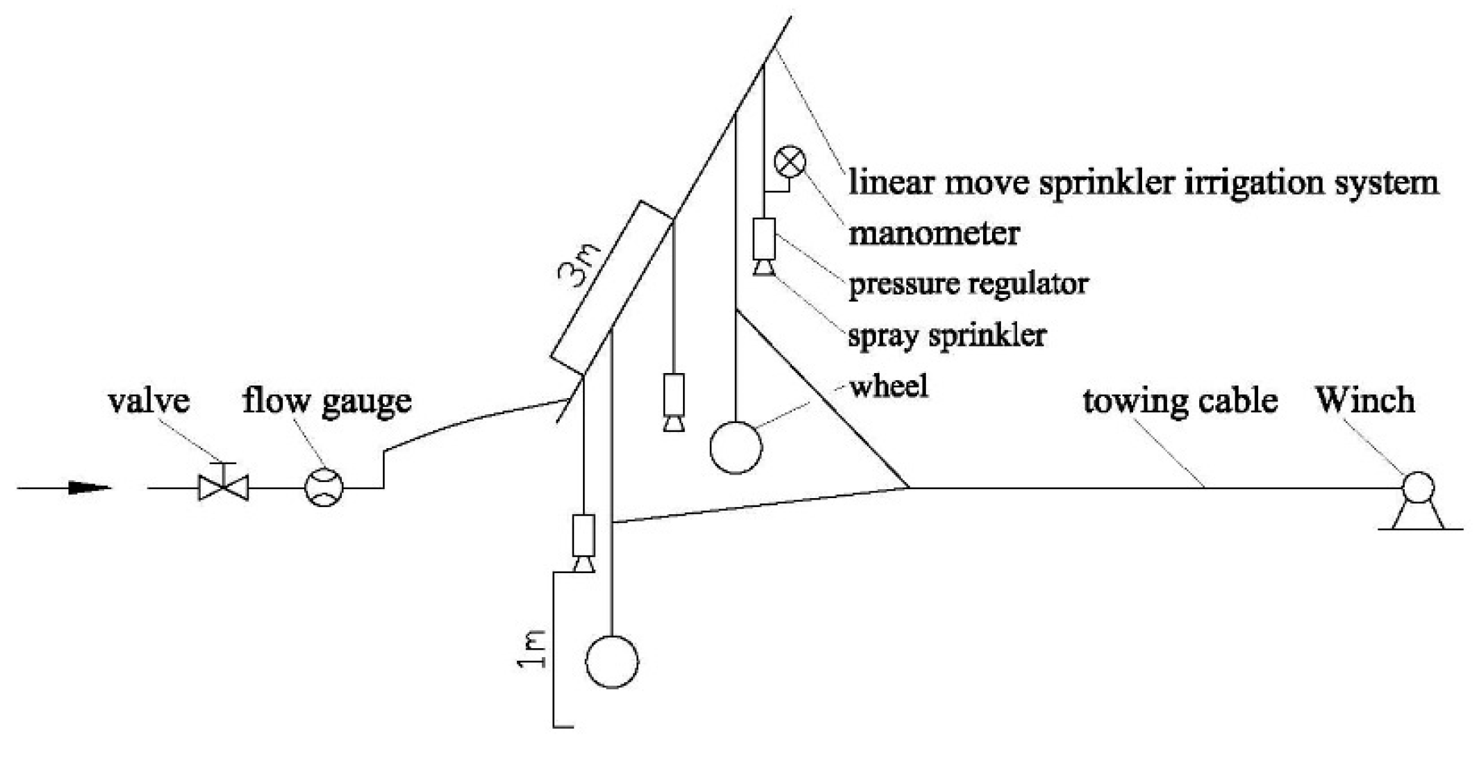
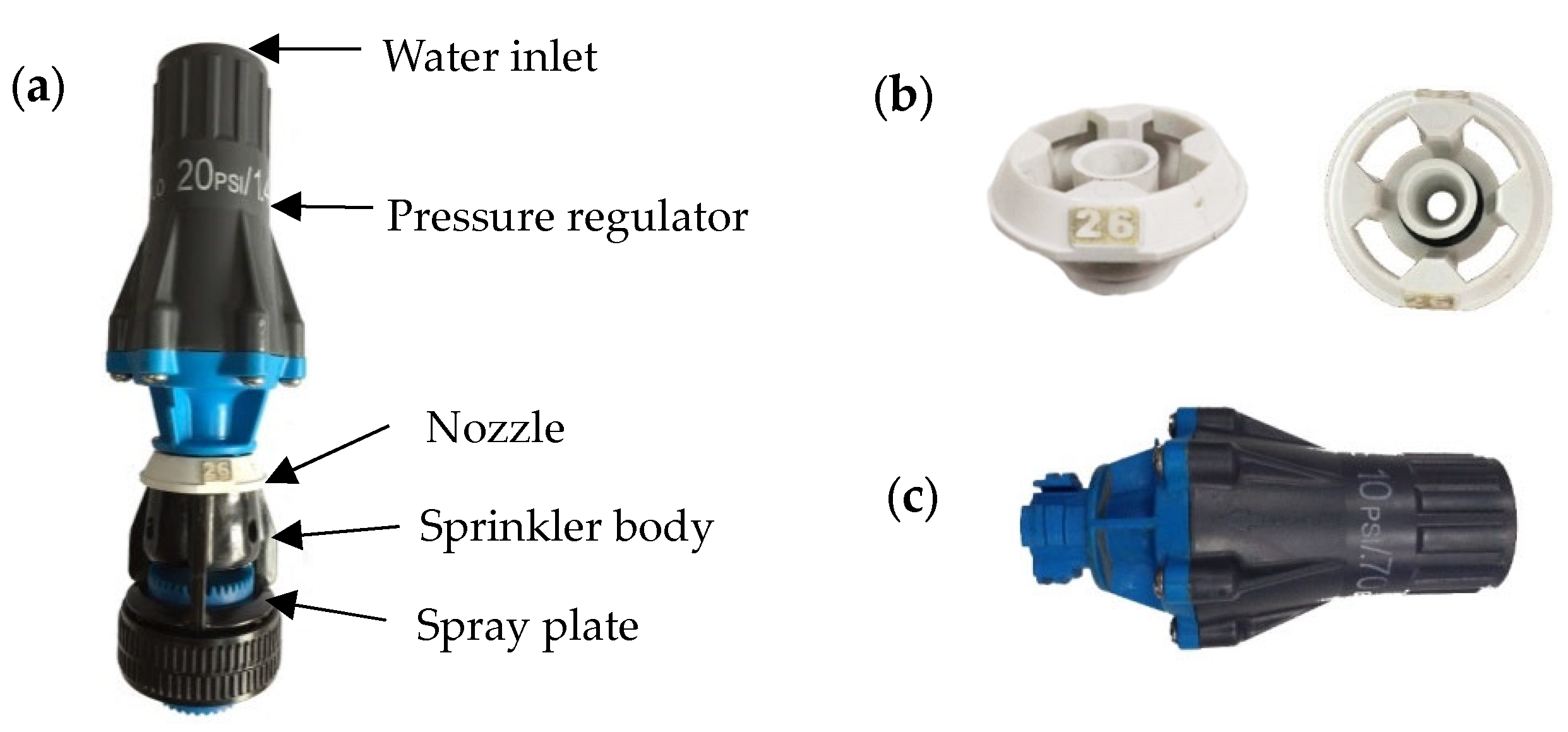
The sprinkler irrigation system used in this study was specifically manufactured as an experimental sample by the Research Center of Fluid Machinery Engineering and Technology (Jiangsu University, Zhenjiang City, Jiangsu Province, China). It was an intermittent linear moving system towed by a winch and installed with a fixed spraying plate package as shown in Figure 1. The fixed spray plate sprinkler studied in this research was the Nelson D 3000 sprayhead (Nelson Irrigation Co., Walla Walla WA, USA). A single-strut pressure regulator (Figure 2a) was part of the package for a low-pressure deflection sprinkler. The shapes of the nozzles were circular (Figure 2b). The nozzle diameter of the fixed spray plate sprinkler was 5.16 mm, corresponding to number #26 specified by the Nelson Company. The sprinkler deflects 36 water streams uniformly, centered from itself, to form a full-circle spray pattern. The pressure regulator and sprinkler were connected immediately with a dedicated screw-type connector (Figure 2c). The reason for using such sprinklers was that prior tests had shown that this package and pressure combination had a good coefficient of uniformity [31,32,33]. All sprinklers were on flexible drop hoses that set the D 3000 sprayhead approximately 1.0 m above the soil surface, and spaced 3.0 m apart. A pressure regulator of 10 or 20 psi (69 or 138 kPa) was installed just upstream of the spray sprinkler. The discharge of the LMIS was measured with an electrical flow gauge (Model E-mag/DN25, manufactured by Kaifeng Electronic Instrument Company, China) with an accuracy of 0.3%.
2.2. Modeling for Calculation of Application Depth
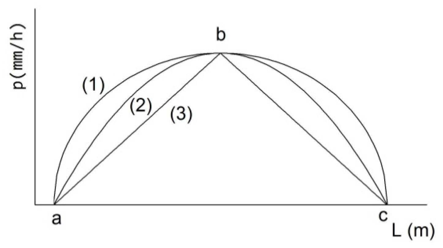
As the structure parameters of sprinkler type, installed height and spacing were determined, with the water distribution along the axis direction of the LMIS known. First, the LMIS was maintained at a constant working condition. Then, according to the maximum wetted radius, R max, and the water application rate of the sprinklers, the figure of water application depth could be obtained. The relationship between the water application and spraying distance may be described by a geometric pattern. An elliptical, parabolic or triangular pattern was chosen to represent it as shown in Figure 3, where the curve of abc represents the distribution line of sprinkler irrigation intensity, the vertical axis represents the water application rate p (mm/h), and the horizontal axis represents the spraying distance L (m). In theory, under the conditions of an indoor experiment without any wind effects, the value of L is two times the maximum wetted radius, R max.
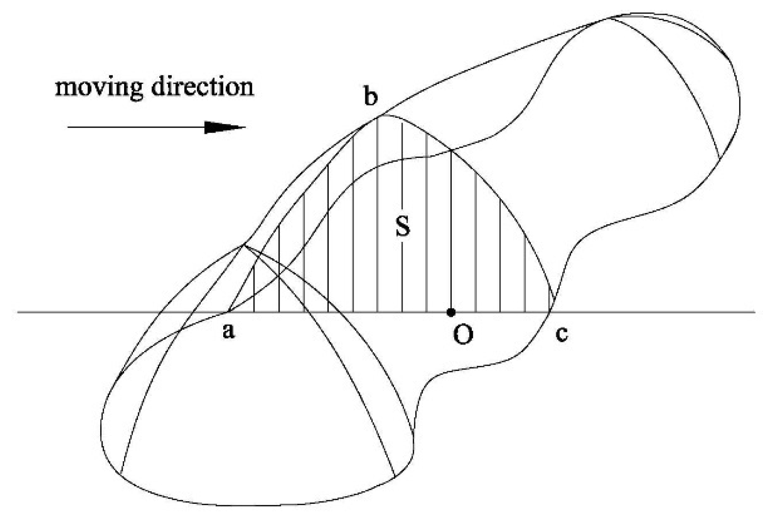
The catch device was supposed to be set at point O, away from the LMIS, with a distance larger than R max, to study the average application depth of the system. The working phenomenon was as following: first, the LMIS approached point O, and point O started to receive the water sprayed out by the LMIS; then, the LMIS gradually receded from point O while moving until the system passed over the catch devices entirely and point O did not receive any water. The LMIS-fulfilled total water application depth was the sum of passing section area of point O. Figure 4 represents the depiction of water application distribution of point O. Combined with Figure 3, when the LMIS was passing through point O at a speed of v, it means that the curve of abc was passing through point O at a speed of v and the passing time could be calculated as t = Lac/v.
At this time, the curve of abc also represents the distribution line of sprinkler irrigation intensity, and the vertical axis also represents the water application rate p (mm/h); however, the horizontal axis represents the passing time t (s). When the LMIS was passing through any point of O, the receiving water of point O was the sum of the water application section area passing point O. Figure 4 represents the distribution section S, and S is the superimposed distribution map of all water sprayed to point O. When the travel speed is v, it can be seen that t = Lac/v. The relationship between the water application rate and the passing through time T was as follows:
Elliptical shape:
Parabolic shape:
Triangular shape:
where
- = peak water application rate (mm h−1)
- t = water application time (h).
Then, the wetted area S was calculated as follows:
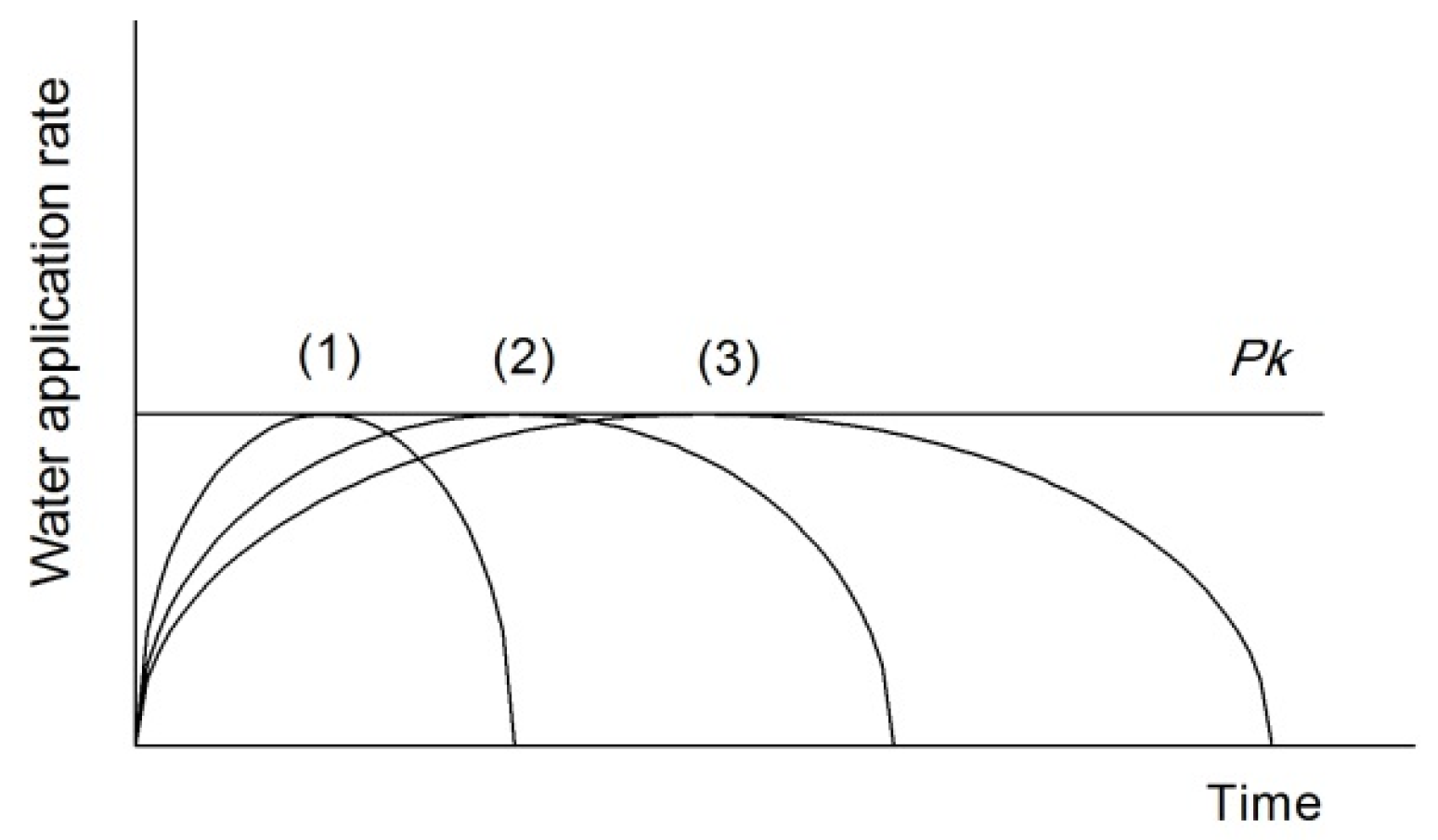
Supposing that the travel speed of LMIS was set at different values of v1, v2, and vn, respectively, t1 = Lac/v1, t2 = Lac/v2, and tn = Lac/vn. The parabolic pattern was selected and was assumed to be representative of LMIS irrigation water, whose pattern for the same water application depth and time has a peak rate between the elliptical and triangular patterns. Figure 5 shows an elliptical application shape. Notice the increase of water application depth (proportional to larger geometric areas) related to high speed, average speed, and low speed, as well as the constant peak water application rate.
2.3. Modeling for Calculation of Uniformity
The spraying irrigation state of LMIS can be regarded as a limit state of mobile spraying for fixed-type pipe with an infinite narrow width. Supposing that the LMIS traveled at a uniform speed, and the water distribution for every sprinkler was the same and does not change with time, it could be determined that the depth of irrigation water along the direction of the sprinkler is the same. Therefore, only the branch direction sprinkling uniformity degree needed to be considered, which can be representative of the entire area of the spraying uniformity. In this way, the concept of linear spraying uniformity is put forward. The uniformity of the LMIS is equal to the uniformity of the axial direction of the unit. The coefficient of uniformity CU (%), developed by Christiansen (1942), was calculated using the following equation:
When the point was adopted by affirmative grid,
where = water depth of calculated point i, mm/h; = mean water depth of all calculated points, mm/h; and n = total number of calculated points used in the evaluation.
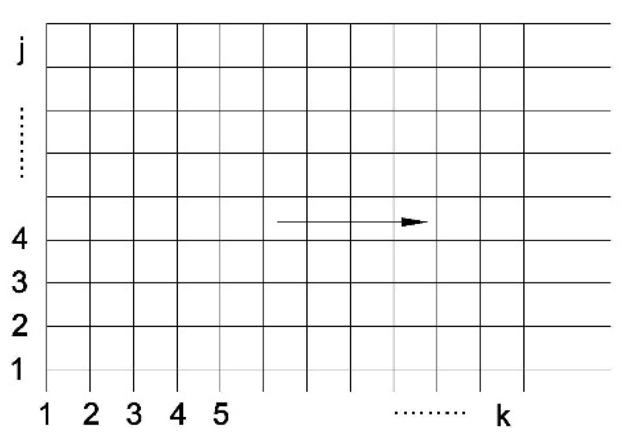
Figure 6 represents the calculated sketch of spraying uniformity for LMIS. The K direction is the running direction and the j direction is the axial of the unit. The water depth of hjk was as follows:
Here, has been simplified to the average value of the depth of the axial point irrigation water.
In the same way:
This type has also been turned into an axial . The spray uniformity coefficient can be obtained after substitution of the axial and into Equation (5).
2.4. Setup and Procedures of Indoor Experiment
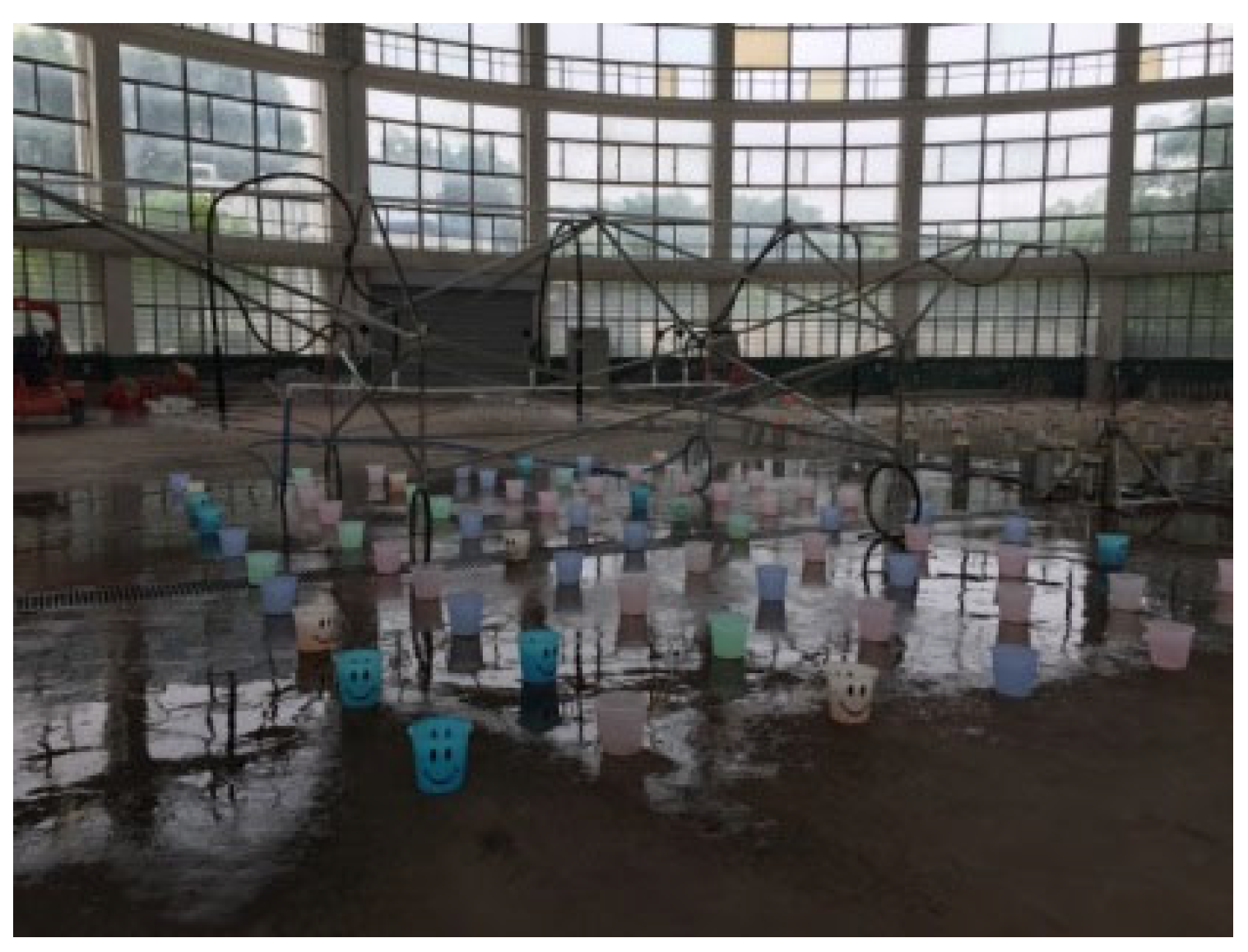
The study site was located at the indoor facilities of the Research Center of Fluid Machinery Engineering and Technology, Jiangsu University (Jiangsu Province, China). Figure 7 shows the test plot for the LMIS mobile water distribution. The structure, built with several metal 40-mm-long and 20-mm-wide rectangular bars, was 12.0 m wide and the spray sprinkler could be adjusted from 0 to 2.5 m above the surface. Because only a short width (12.0 m) was tested, pressure variation through the measured width of the system was assumed to be negligible. The frame corners were equipped with four wheels and a winch was used to tow the system. The water source was a reservoir with a capacity of 60 m3. A 3.0-kW electric centrifugal pump was connected to the water supplying pipe and a 36-mm external-diameter hose pipe was used to supply water to the spray sprinkler. Manometers and valves were installed as required to control water supply during the experiments (as shown in Figure 1). Catch cans were used to collect the applied water. They were constructed from transparent plastic, with an inverted conical shape. The catch can opening was 200 mm for the inside diameter and the catch can height was 250 mm. Nine rows of catch cans were distributed along the direction of the vertical moving unit, and the distance and spacing of catch cans were 1 m each. The LMIS and the catch cans were installed in a plot with cement flooring. After the spraying test, the weighing method was used to calculate the depth of irrigation water for every catch can. The measured irrigation depth of the point values was taken with an average irrigation depth of the 9 rows of catch cans.
Experiments were carried out at a constant pressure of 69 and 138 kPa, respectively, maintained by a 10- and 20-psi pressure regulator. The pulsing frequency towed by the winch was 1.0 cycle/min while operating the winch at percent-timer settings of 30, 45, 60, 75%, and 90%, corresponding to the average moving speed of 1.5, 2.3, 3.3, 4.0, and 4.7 m min−1, respectively. These selected five values cover the range of duty cycles that are expected to be used in the field. A value of 100% is the same as normal operating conditions (constant sprinkler discharge) and zero percent is the same as operating the system dry. All operating pressures and moving speeds were within the manufacturer’s recommendations. The following standards [34,35,36,37] were adopted in the design of the experimental setup and in the experiment itself. The duration of each test was approximately 30 to 45 min. The applied water in the catch cans was read in a measuring cup with a volume of 500 mL and an accuracy of 5 mL. The read data were then converted to average irrigation depth by dividing the cross-sectional area of the catch can. A minimum of three replications were conducted for each pressure and moving speed combination, and data were averaged and used as the final experimental data. Flow rates from the two operating pressures used for the application depth tests were measured three times under the same operating conditions. A metal pipe was positioned over the sprinkler nozzles and the discharge water directed into a bucket for 2 min. Discharge volumes were then weighed with an electronic balance (Otimpa Corp, China) with 1 gram accuracy and converted into flow rate.
The average air temperature during testing was 20.8 °C and ranged from 17.8 °C to 22.4 °C. The average relative humidity was 41% and ranged from 36% to 47%. To verify the accuracy of the model, a moving superposed water quantity verification test was carried out. Taking into account the condition that the work at the beginning of the LMIS may not be stable, the moving procedure of the system was start-up and test data were collected after operating at the working pressure for more than 10 min.
3. Results and Discussion
The stable working state of the LMIS means the spraying speed is stable, and the working pressure of the spray head on the system is stable. The wind speed during the entire tests ranged from 0.0 to 0.12 m s−1 and was usually less than 0.1 m s−1. These data are not presented or discussed as the values were less than the lower threshold of the measuring equipment. The potential source of error in this study is any differences in evaporative conditions across the time period of the various tests. Although many studies have been conducted on evaporation during sprinkler irrigation, Schneider [38] noted that no more than 2% losses resulted from evaporation during use of sprinkler irrigation systems. For example, even under a condition of an average temperature of 26 °C, a relative humidity of 64%, and a wind speed of 6.4 m/s, the measured evaporation was only 0.8% of total sprinkler discharge [39]. Therefore, due to the indoor experimental conditions without any wind effects in the study, this particular potential source of error was minimized. An indoor experiment was conducted to verify the accuracy of the model using the Nelson D 3000 spray head with a nozzle diameter of 5.16 mm at working pressures of 69 kPa and 138 kPa and at an elevation of 1.0 m above the soil surface.
3.1. Coefficient of Discharge
The results of measured flow rates of sprinkler irrigation nozzles used in this study are shown in Table 1. Analysis of the measured data were performed to find the influence of the geometrical parameters as well as the operating pressure on discharge of the sprinkler head, which can be expressed in terms of the discharge coefficient, C. The coefficient of discharge of the sprinkler is generally expressed as follows:
where C is the coefficient of discharge, Q is the flow rate of the sprinkler (m3 h−1), d is the diameter of the nozzle (m), g is the gravitational acceleration (m s−2), and H is the pressure head (m).
As shown in Table 1, when using the fixed spray plate sprinkler, the measured nozzle flow rates ranged from 0.77 to 0.84 m3 h−1, with a mean value of 0.808 m3 h−1, and 1.15 to 1.22 m3 h−1 with a mean value of 1.183 m3 h−1 for the pressure regulators of specification 69 and 138 kPa, respectively. After calculating using Equation (8), the nozzle coefficients of discharge ranged from 0.880 to 0.960 with a mean value of 0.923, and 0.929 to 0.986 with a mean value of 0.956, for 69 and 138 kPa, respectively. From the aforementioned analysis, it was found that the coefficients of discharge fluctuated within a small acceptable range under the same operating pressure, which could be attributed to the acceptable experimental error. Additionally, the coefficients of discharge obtained using the 138 kPa pressure regulator were higher than those obtained using the 69 kPa pressure regulator, which means that using a pressure regulator with a higher outlet pressure produced higher coefficients of discharge.
3.2. Measured Water Distributions
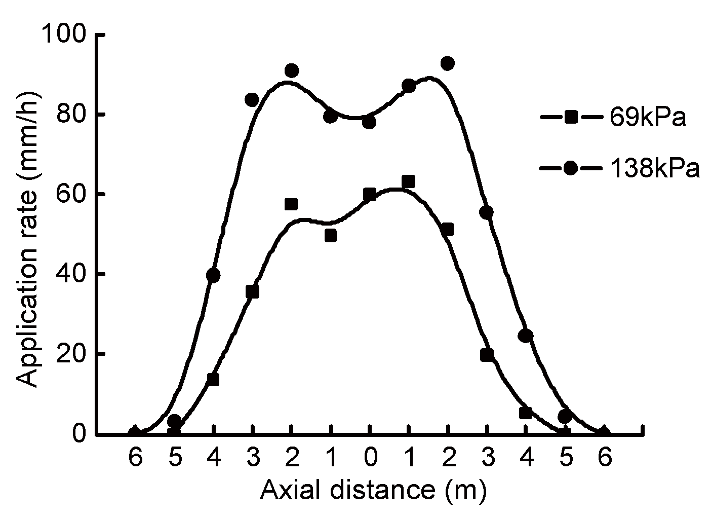
Figure 8 represents the measured sprinkler intensity and fitting curve of radial points with a nozzle diameter of 5.16 mm and a height of 1.0 m at operating pressures of 69 kPa and 138 kPa, respectively.
As shown in Figure 8, the sprinkler nozzle wetting radius for 69 kPa and 138 kPa was 4.4 m and 5.7 m, respectively. The sprinkler head produced quite similar water application profiles under different operating pressures. The average values of the sprinkler head application rates varied from 3.2 mm h−1 to 92.8 mm h−1. The water application rate increased to a maximum value first and then decreased approximately linearly as the distance from the sprinkler increased. The maximum application rate was determined for the two analyzed pressures: 63.2 mm h−1 at distances of 1 m for 69 kPa, and 92.8 mm h−1 at 2 m from the sprinkler for 138 kPa. Starting from this distance, the application rate decreased until it reached the minima. For 69 kPa at 4 m, and 138 kPa at 5 m, the minimum values were 5.3 and 4.3 mm h−1, respectively. The application rates had large variability for all measured points. The applied water depths were extremely similar to the radial water depths, indicating that the water distribution pattern of individual sprinklers had a primary influence on the overall water application depth and distribution uniformity. The radial water distribution curve appeared as a saddle type, and had two sprinkler intensity peaks close to the sprinkler. The least squares method was used for curve fitting to simulate the water distribution characteristics, and the fitting degree was as high as 0.89. Table 2 summarizes the measured application depths and corresponding CU values obtained with an LMIS average moving speed of 1.5, 2.3, 3.3, 4.0 and 4.7 m/min under different operating pressures of 69 kPa and 138 kPa. For the various LMIS speeds, the application depth of 69 kPa varied from 1.3 to 4.2 mm with an average of 2.38 mm, the CU varied from 84.5% to 88.9% with an average of 86.58%, and the standard deviation had an average of 0.16; the application depth of 138 kPa varied from 2.6 to 7.7 mm with an average of 4.08 mm, the CU varied from 85.9% to 89.8% with an average of 87.28%, and the standard deviation had an average of 0.68. It appeared that the application depth decreased as the LMIS speed increased, which could be understood easily. The CU value did not linearly relate to the LMIS speed, which was interpreted as adjusting for unimportant variability on a small scale.
3.3. Comparison of Application Depth and CU Values between Experimental Measured Data and Modeling Simulations
As shown in Section 2.2 and Section 2.3, in the modeling for calculation of application depth and CU values of the sprinkler irrigation, the data from Figure 8 were used as the basic foundation, and the fitting curves were supposed to be regulated as elliptical, parabolic, and triangular shapes, respectively.
3.3.1. Application Depth
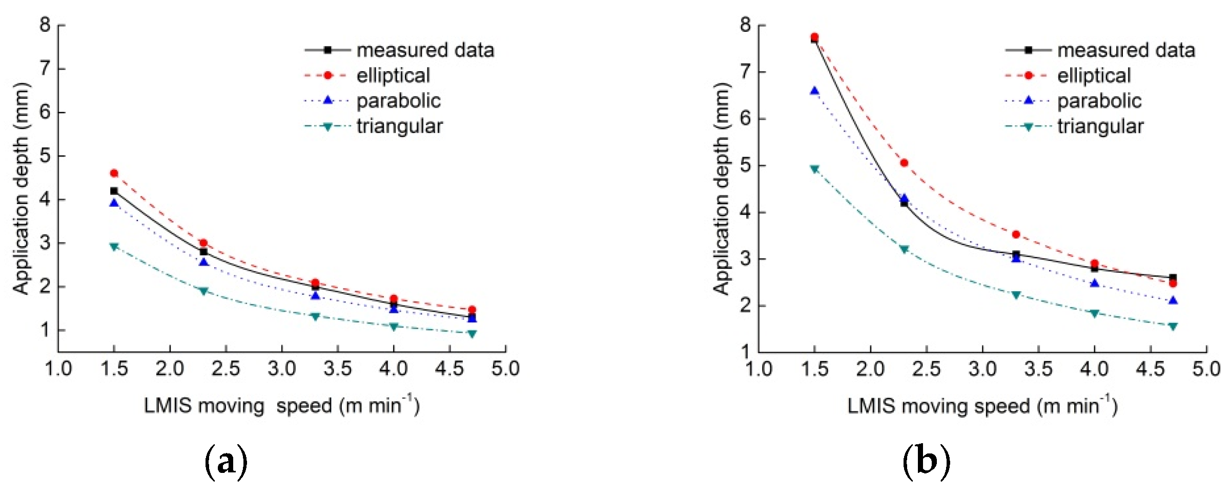
The simulated application depths were obtained with a constant spacing of 3.0 m for comparison. The data from Table 2 were used as the experimental measured data. As a further illustration of model validation of the application depth calculation, Figure 9 presents a comparison of application depth between measured data and model-simulated results at an operating pressure of 69 kPa and 138 kPa, respectively.
As seen from Figure 9, there appears agreement between the measured and simulated mean application depths. The measured data and model-simulated application depths for all the elliptical-, parabolic-, and triangular-shaped predictions decreased with an increasing average moving speed, which was in accordance with the analysis that slower moving speeds will result in more spraying water. The measured application depths were much larger than the triangular-shaped prediction simulated application depths and were just between the parabolic-shaped prediction and the elliptical-shaped prediction simulated application depths.
Compared to the experimental measured data at an operating pressure of 69 kPa, the simulated result was from 28.0% to 33.3% lower with an average of 30.9% for the triangular-shaped prediction, from 4.0% to 11.1% lower with an average of 7.8% for the parabolic-shaped prediction, and from 4.7% to 13.1% higher with an average of 8.5% for the elliptical-shaped prediction, respectively. Compared to the experimental measured data at an operating pressure of 138 kPa, the simulated result was from 23.3% to 39.3% lower with an average of 32.0% for the triangular-shaped prediction, from 2.3% to 19.1% lower with an average of 10.2% for the parabolic-shaped prediction, and from 3.9% to 20.4% higher with an average of 8.7% for the elliptical-shaped prediction, respectively. Normally, the measured water depth is generally a slight deviation from the calculated value, caused by the fitting error, the testing error, evaporation and drift during the spraying process [40,41,42]. Therefore, it was determined that both the parabolic- and elliptical-shaped predictions were the acceptable shapes of the water distribution pattern, as they were closer to the measured application depth.
The measured application depth and model-simulated results based on overlapping the measured water distribution data of individual sprinklers were curved lines. Special attention was given to the development of empirical equations for water application depth with regard to moving speed. The curvilinear Equation (10) was regressed and Table 3 presents the equations of those profiles. The coefficient of determination (R2) for measured data ranged from 0.9698 to 0.9954 and for all the model simulations was 0.9946.
where p is the application depth (mm) and v is the LMIS speed (m min−1).
3.3.2. Coefficient of Uniformity
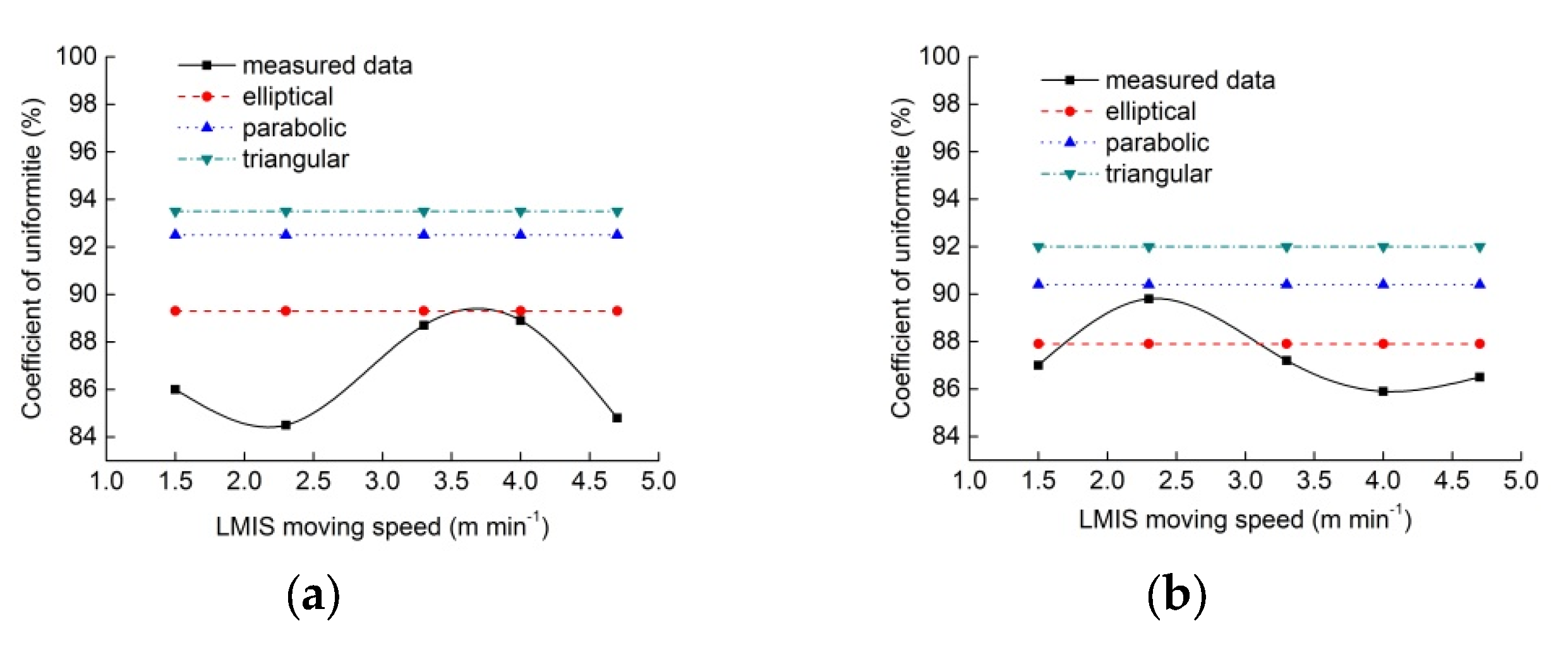
The simulated CU values were obtained using MATLAB calculations based on the basic foundation of application depth values from Figure 9. The combined CU values were calculated using the aforementioned method. The data from Table 2 were used as the experimental measured data. As a further illustration of model validation of CU calculations, Figure 10 presents the comparison of CU between experimental measured data and model-simulated results at an operating pressure of 69 kPa and 138 kPa, respectively.
As seen in Figure 10, there appears agreement between the measured and simulated CU values. The simulated CU for all the elliptical-, parabolic-, and triangular-shaped predictions maintains a constant value and does not vary with increasing speed. It was determined that a different moving speed has an influence on the depth of irrigation water along the direction of the sprinkler, which varies at a same percentage and does not affect CU values; only the branch direction data affect the sprinkling CU degrees, which can be representative of the entire area of the spraying uniformity. Therefore, when the branch water distribution shape was determined as an elliptical, parabolic, or triangular prediction, the simulated CU keeps a constant value at different moving speeds. However, the measured CUs were variable for all moving speeds. The range of combined CU values at different pressures were as follows: 84.5% at a moving speed of 2.3 m min–1 to 88.9% at a moving speed of 4.0 m min–1 (69 kPa), and 85.9% at a moving speed of 4.0 m min–1 to 89.8% at moving speed of 2.3 m min–1 (138 kPa). It was determined that the measured CU values with regard to moving speed fluctuated within a small range, and could be attributed to the acceptable fitting and experimental error.
Compared to the experimental measured data at an operating pressure of 69 kPa, the simulated CU value was 93.5% and of an absolute deviation rate from 5.2% to 10.7% with an average of 8.0% for the triangular-shaped prediction, 92.5% and of an absolute deviation rate from 4.0% to 9.5% with an average of 6.9% for the parabolic-shaped prediction, and 89.3% and of an absolute deviation rate from 0.4% to 5.7% with an average of 3.2% for the elliptical-shaped prediction, respectively. Compared to the experimental measured data at an operating pressure of 138 kPa, the simulated CU value was 92.0% and of an absolute deviation rate from 2.4% to 7.1% with an average of 5.4% for the triangular-shaped prediction, 90.4% and of an absolute deviation rate from 0.7% to 5.2% with an average of 3.6% for the parabolic-shaped prediction, and 87.9% and of an absolute deviation rate from 0.8% to 2.3% with an average of 1.6% for the elliptical-shaped prediction, respectively.
From the aforementioned analysis, it was determined that for the parabolic- and elliptical-shaped predictions, the deviations of the points are within 5% except for several cases at a moving speed of 2.3 and 4.0 m min–1. This deviation may result from inaccurate measurement of the effective wetted widths. Generally, the simplified model has a high computational accuracy, which could be brought into Equation (5) to further calculate the LMIS spraying uniformity. The comparison of measured and model-simulated data indicated that the measured water distribution pattern of individual sprinklers could be represented both as an elliptical- or parabolic-shaped prediction, which was accurate and reliable for simulating the application performance of the LMIS and verified that the calculation of application depth and CU values shown in this work is applicable in practice.
In short, a new model of the LMIS has been developed and a sprinkler irrigation system was specifically manufactured as an experimental sample to verify the accuracy of the model. The differences in model accuracy owing to different operating pressures were not significant, and the moving speed of the LMIS did not appear to influence model accuracy either. Comparisons between experimental data and model simulations revealed that the model can accurately predict water application depth and CU values along the LMIS. Although the model was developed and validated for linear moving systems, it could be readily used for center pivots, which constitute a simplification of the calculation approach adopted.
4. Conclusions
This study presents a model of application depth and uniformity for the LMIS. Based on the obtained results and the conditions in which this trial was carried out, the following can be concluded:
At an operating pressure of 69 kPa and 138 kPa, the sprinkler nozzle wetting radius was 4.4 m and 5.7 m, respectively. The sprinkler head produced quite similar water application profiles, which appeared as a saddle type and had two sprinkler intensity peaks close to the sprinkler.
Compared to the experimental measured data at operating pressures of 69 kPa or 138 kPa, the simulated application depth was on average 30.9% or 32.0% lower for the triangular-shaped prediction, 7.8% or 10.2% lower for the parabolic-shaped prediction, and 8.5% or 8.7% for the elliptical-shaped prediction, respectively. The curvilinear equations for the measured application depth and model-simulated results were regressed and the coefficient of determination (R2) was from 0.9698 to 0.9954. The simulated CU was an average deviation rate of 8.0% or 5.4% for the triangular-shaped prediction, 6.9% or 3.6% for the parabolic-shaped prediction, and 3.2% or 1.6% for the elliptical-shaped prediction, respectively.
This study indicates that a sprinkler irrigation system for the LMIS that is both elliptical and parabolic in shape could be considered as far as application depths and CU values are concerned. The model can therefore be further developed to provide a useful tool for LMIS design and management.
Author Contributions
J.L. was the supervision of this manuscript; X.Z. was writing the original draft and making all revisions; S.Y. was providing the funding acquisition; and A.F. was doing the literature resources.
Funding
This research was funded by the National Key Research and Development Program of China (No. 2016YFC0400202), the Key R&D Project of Jiangsu Province (Modern Agriculture) (No. BE2018313), and the Priority Academic Program Development of Jiangsu Higher Education Institutions (PAPD).
Acknowledgments
The authors are greatly indebted to the supports from students of the Research Centre of Fluid Machinery and Engineering, Jiangsu University for their assistances in conducting the experiment.
Conflicts of Interest
The authors declare no conflict of interest.
References
- Yuan, S.Q.; Li, H.; Wang, X.K. Status, problems, trends and suggestions for water-saving irrigation equipment in China. J. Drain. Irrig. Mach. Eng. (JDIME) 2015, 33, 78–92. [Google Scholar]
- Zhu, X.Y.; Chikangaise, P.; Shi, W.D.; Chen, W.H.; Yuan, S.Q. Review of intelligent sprinkler irrigation technologies for remote autonomous system. Int. J. Agric. Biol. Eng. 2018, 11, 23–30. [Google Scholar] [CrossRef]
- Xu, D.; Li, Y.N.; Gong, S.H.; Zhang, B.Z. Experiment on sweet pepper nitrogen detection based on near infrared reflectivity spectral ridge regression. J. Drain. Irrig. Mach. Eng. (JDIME) 2019, 37, 63–72. [Google Scholar]
- Hart, W.E. Sprinkler distribution analysis with a digital computer. Trans ASAE 1963, 6, 206–208. [Google Scholar]
- Vories, E.D.; Von Bernuth, R.D. Single nozzle sprinkler performance in wind. Trans. ASAE 1986, 29, 1325–1330. [Google Scholar]
- Li, J.; Kawano, H. Sprinkler rotation nonuniformity and water distribution. Trans. ASAE 1996, 39, 2027–2031. [Google Scholar] [CrossRef]
- Zhu, X.Y.; Yuan, S.Q.; Jiang, J.Y.; Liu, J.P.; Liu, X.F. Comparison of fluidic and impact sprinklers based on hydraulic performance. Irrig. Sci. 2015, 33, 367–374. [Google Scholar] [CrossRef]
- Liu, J.P.; Yuan, S.Q.; Li, H.; Zhu, X.Y. Experimental and combined calculation of variable fluidic sprinkler in agriculture irrigation. AMA-Agr. Mech. Asia Afr. Lat. Am. 2016, 47, 82–88. [Google Scholar]
- Xiang, Q.J.; Xu, Z.D.; Chen, C. Experiments on air and water suction capability of 30PY impact sprinkler. J. Drain. Irrig. Mach. Eng. (JDIME) 2018, 36, 82–87. [Google Scholar]
- Hu, G.; Zhu, X.Y.; Yuan, S.Q.; Zhang, L.G.; Li, Y.F. Comparison of ranges of fluidic sprinkler predicted with BP and RBF neural network models. J. Drain. Irrig. Mach. Eng. (JDIME) 2019, 37, 263–269. [Google Scholar]
- Christiansen, J.E. Irrigation by Sprinkling; Bulletin 670; California Agricultural Experiment Station, University of California: Berkeley, CA, USA, 1942. [Google Scholar]
- Solomon, K. Variability of sprinkler coefficient of uniformity test results. Trans. ASAE 1979, 22, 1078–1080. [Google Scholar] [CrossRef]
- Fukui, Y.; Nakanishi, K.; Okamura, S. Computer evaluation of sprinkler irrigation uniformity. Irrig. Sci. 1980, 2, 23–32. [Google Scholar] [CrossRef]
- Seginer, I.; Kantz, D.; Bernuth, R.D. Indoor measurement of single-radius sprinkler patterns. Trans. ASAE 1992, 35, 523–533. [Google Scholar] [CrossRef]
- Tarjuelo, J.M.; Montero, J.; Valiente, M.; Honrubia, F.T.; Ortiz, J. Irrigation uniformity with medium size sprinklers. Part I: Characterization of water distribution in no-wind conditions. Trans. ASAE 1999, 42, 665–675. [Google Scholar] [CrossRef]
- Michael, J.L.; John, S.S. Sprinkler head maintenance effects on water application uniformity. J. Irrig. Drain. Eng. ASCE 2000, 126, 142–148. [Google Scholar]
- Playán, E.; Zapata, N.; Faci, J.M.; Tolosa, D.; Lacueva, J.L.; Pelegrin, J.; Salvador, R.; Sanchez, I.; Lafita, A. Assessing sprinkler irrigation uniformity using a ballistic simulation model. Agric. Water Manag. 2006, 84, 89–100. [Google Scholar] [CrossRef]
- Zhu, X.Y.; Yuan, S.Q.; Liu, J.P. Effect of sprinkler head geometrical parameters on hydraulic performance of fluidic sprinkler. J. Irrig. Drain. Eng. ASCE 2012, 138, 1019–1026. [Google Scholar] [CrossRef]
- Zhang, L.; Merkley, G.P.; Pinthong, K. Assessing whole-field sprinkler irrigation application uniformity. Irrig. Sci. 2013, 31, 87–105. [Google Scholar] [CrossRef]
- Liu, J.P.; Yuan, S.Q.; Darko, R.O. Characteristics of water and droplet size distributions from fluidic sprinklers. Irrig. Drain. 2016, 65, 522–529. [Google Scholar] [CrossRef]
- Yuan, S.Q.; Darko, R.O.; Zhu, X.Y.; Liu, J.P.; Tian, K. Optimization of movable irrigation system and performance assessment of distribution uniformity under varying conditions. Int. J. Agric. Biol. Eng. 2017, 10, 72–79. [Google Scholar]
- Tang, L.D.; Yuan, S.Q.; Qiu, Z.P. Development and research status of water turbine for hose reel irrigator. J. Drain. Irrig. Mach. Eng. (JDIME) 2018, 36, 963–968. [Google Scholar]
- Lu, M.Y.; Lu, K.J.; Hu, G.; Zhu, X.Y. Experiment on hydraulic performance of type SD-03 pop-up sprinkler. J. Drain. Irrig. Mach. Eng. (JDIME) 2018, 36, 1120–1124. [Google Scholar]
- Buchleiter, G.W. Performance of LEPA equipment on center pivot machines. Appl. Eng. Agric. 1992, 8, 631–637. [Google Scholar] [CrossRef]
- King, B.A.; Kincaid, D.C. Optimal performance from center pivot sprinkler systems. Trans. ASABE 1995, 38, 1737–1747. [Google Scholar]
- Luz, P.B. A graphical solution to estimate potential runoff in center-pivot irrigation. Trans. ASABE 2011, 54, 81–92. [Google Scholar] [CrossRef]
- Martin, D.L.; Kranz, W.L.; Thompson, A.L.; Liang, H. Selecting sprinkler packages for center pivots. Trans. ASABE 2012, 55, 513–523. [Google Scholar] [CrossRef]
- Lu, J.; Cheng, J. Numerical simulation analysis of energy conversion in hydraulic turbine of hose reel irrigator JP75. J. Drain. Irrig. Mach. Eng. (JDIME) 2018, 36, 448–453. [Google Scholar]
- Zhu, X.Y.; Peters, T.; Neibling, H. Hydraulic performance assessment of LESA at low pressure. Irrig. Drain. 2016, 65, 530–536. [Google Scholar] [CrossRef]
- Tian, K.; Zhu, X.Y.; Wan, J.H.; Bao, Y. Development and performance test of lateral move irrigation system. J. Drain. Irrig. Mach. Eng. (JDIME) 2017, 35, 357–361. [Google Scholar]
- Yan, H.J.; Jin, H.Z. Study on the discharge coefficient of nonrotatable sprays for center-pivot system. J. Irrig. Drain. Eng. ASCE 2004, 23, 55–58. [Google Scholar]
- Dogana, E.; Kirnaka, H.; Dogan, Z. Effect of varying the distance of collectors below a sprinkler head and travel speed on measurements of mean water depth and uniformity for a linear move irrigation sprinkler system. Biosyst. Eng. 2008, 99, 190–195. [Google Scholar] [CrossRef]
- Yan, H.J.; Jin, H.Z.; Qian, Y.C. Characterizing center pivot irrigation with fixed spray plate sprinklers. Sci. Chin. 2010, 53, 1398–1405. [Google Scholar] [CrossRef]
- ASAE Standards. Procedure for Sprinkler Distribution Testing for Research Purposes, 32nd ed.; S330.1; ASAE: St. Joseph, MI, USA, 1985. [Google Scholar]
- ASAE Standards. Procedure for Sprinkler Testing and Performance Reporting, 32nd ed.; S398.1; ASAE: St. Joseph, MI, USA, 1985. [Google Scholar]
- ASAE. Test Procedure for Determining the Uniformity of Water Distribution of Center Pivot and Lateral Move Irrigation Machines Equipped with Spray or Sprinkler Nozzles; ANSI/ASAE S436.1 MAR01; ASAE Standards: St. Joseph, MI, USA, 2001. [Google Scholar]
- MOD GB/T 19795.2. Agricultural Irrigation Equipment—Rotating Sprinklers—Part 2: Uniformity of Distribution and Test Methods; International Organization for Standardization: Geneva, Switzerland, 2005. [Google Scholar]
- Schneider, A.D. Efficiency and uniformity of the LEPA and spray sprinkler methods: A review. Trans. ASAE 2000, 43, 937–944. [Google Scholar] [CrossRef]
- Kohl, K.D.; Kohl, R.A.; DeBoer, D.W. Measurement of low pressure sprinkler evaporation loss. Trans. ASAE 1987, 30, 1071–1074. [Google Scholar] [CrossRef]
- Dechmi, F.; Playán, E.; Cavero, J.; Faci, J.M.; Martínez-Cob, A. Wind effects on solid set sprinkler irrigation depth and yield of maize (Zea mays). Irrig. Sci. 2003, 22, 67–77. [Google Scholar] [CrossRef]
- Playán, E.; Salvador, R.; Faci, J.M. Day and night wind drift and evaporation losses in sprinkler solid-sets and moving laterals. Agric. Water Manag. 2005, 76, 139–159. [Google Scholar] [CrossRef]
- Zhang, M.; Zhao, W.X.; Li, J.S.; Li, Y.F. Fertigation uniformity and evaporation drift losses of center pivot irrigation system. J. Drain. Irrig. Mach. Eng. (JDIME) 2018, 36, 1125–1130. [Google Scholar]
Figure 1.
Description of the linearly moved irrigation system (LMIS).

Figure 2.
Pressure regulator and sprinkler used in the LMIS (a), nozzles used in the sprinkler (b), and dedicated screw-type connector of pressure regulator (c).
Figure 2.
Pressure regulator and sprinkler used in the LMIS (a), nozzles used in the sprinkler (b), and dedicated screw-type connector of pressure regulator (c).

Figure 3.
Water application depth: (1) elliptical, (2) parabolic and (3) triangular.

Figure 4.
Depiction of water application distribution of point O.

Figure 5.
Water application patterns with decreasing speed at the same irrigation point: (1) high speed, (2) average speed, and (3) low speed.
Figure 5.
Water application patterns with decreasing speed at the same irrigation point: (1) high speed, (2) average speed, and (3) low speed.

Figure 6.
Calculated sketch of spraying uniformity for the LMIS.

Figure 7.
Test plot for the LMIS mobile water distribution.

Figure 8.
Measured radial application rate and fitting curve for operating pressures of 69 kPa and 138 kPa.
Figure 8.
Measured radial application rate and fitting curve for operating pressures of 69 kPa and 138 kPa.

Figure 9.
Comparison of application depth between experimental measured data and model-simulated results: (a) 69 kPa, (b) 138 kPa.
Figure 9.
Comparison of application depth between experimental measured data and model-simulated results: (a) 69 kPa, (b) 138 kPa.

Figure 10.
Comparison of CU between experimental measured data and model-simulated results. (a) 69 kPa, (b) 138 kPa.
Figure 10.
Comparison of CU between experimental measured data and model-simulated results. (a) 69 kPa, (b) 138 kPa.


Table 1.
Measured flow rates of sprinkler irrigation nozzles.
| 69 kPa | 138 kPa | ||||||
|---|---|---|---|---|---|---|---|
| Flow Rate, m3 h−1 | Nozzle I | Nozzle II | Nozzle III | Nozzle I | Nozzle II | Nozzle III | |
| Replications | |||||||
| 1 | 0.8 | 0.79 | 0.8 | 1.16 | 1.21 | 1.22 | |
| 2 | 0.84 | 0.83 | 0.81 | 1.18 | 1.17 | 1.15 | |
| 3 | 0.77 | 0.8 | 0.83 | 1.21 | 1.16 | 1.19 | |
| Mean | 0.80 | 0.81 | 0.81 | 1.18 | 1.18 | 1.19 | |
Table 2.
Measured irrigation application depths and corresponding coefficient of uniformities under different operating pressures and LMIS speeds.
Table 2.
Measured irrigation application depths and corresponding coefficient of uniformities under different operating pressures and LMIS speeds.
| Operating Pressure (kPa) | LMIS Speed (m min−1) | Application Depth (mm) | CU (%) | Standard Deviation |
|---|---|---|---|---|
| 69 kPa | 1.5 | 4.2 | 86.0 | 0.15 |
| 2.3 | 2.8 | 84.5 | 0.26 | |
| 3.3 | 2.0 | 88.7 | 0.12 | |
| 4.0 | 1.6 | 88.9 | 0.12 | |
| 4.7 | 1.3 | 84.8 | 0.15 | |
| Mean | 2.38 | 86.58 | 0.16 | |
| 138 kPa | 1.5 | 7.7 | 87.0 | 0.75 |
| 2.3 | 4.2 | 89.8 | 0.82 | |
| 3.3 | 3.1 | 87.2 | 1.00 | |
| 4.0 | 2.8 | 85.9 | 0.47 | |
| 4.7 | 2.6 | 86.5 | 0.36 | |
| Mean | 4.08 | 87.28 | 0.68 |
Table 3.
Equations of water application depth with regard to moving speed.
| 69 kPa | 138 kPa | |||||||
|---|---|---|---|---|---|---|---|---|
| A | B | C | R2 | A | B | C | R2 | |
| Measured data | 0.186 | 1.814 | 5.780 | 0.9954 | 0.529 | 4.331 | 11.26 | 0.9698 |
| Elliptical prediction | 0.231 | 2.140 | 6.461 | 0.9946 | 0.389 | 3.605 | 10.88 | 0.9946 |
| Parabolic prediction | 0.196 | 1.818 | 5.487 | 0.9946 | 0.330 | 3.061 | 9.240 | 0.9946 |
| Triangular prediction | 0.147 | 1.363 | 4.115 | 0.9946 | 0.248 | 2.300 | 6.930 | 0.9946 |
© 2019 by the authors. Licensee MDPI, Basel, Switzerland. This article is an open access article distributed under the terms and conditions of the Creative Commons Attribution (CC BY) license (http://creativecommons.org/licenses/by/4.0/).
Share and Cite
MDPI and ACS Style
Liu, J.; Zhu, X.; Yuan, S.; Fordjour, A. Modeling the Application Depth and Water Distribution Uniformity of a Linearly Moved Irrigation System. Water 2019, 11, 827. https://doi.org/10.3390/w11040827
AMA Style
Liu J, Zhu X, Yuan S, Fordjour A. Modeling the Application Depth and Water Distribution Uniformity of a Linearly Moved Irrigation System. Water. 2019; 11(4):827. https://doi.org/10.3390/w11040827
Chicago/Turabian StyleLiu, Junping, Xingye Zhu, Shouqi Yuan, and Alexander Fordjour. 2019. "Modeling the Application Depth and Water Distribution Uniformity of a Linearly Moved Irrigation System" Water 11, no. 4: 827. https://doi.org/10.3390/w11040827
Note that from the first issue of 2016, this journal uses article numbers instead of page numbers. See further details here.