Soil Water Dynamics in a Rainfed Mediterranean Agricultural System


1
Department of Environment and Soil Sciences, University of Lleida, Avinguda Alcalde Rovira Roure 191, E-25198, 25003 Lleida, Spain
2
Research Institute of Water and Environmental Engineering (IIAMA), Universitat Politècnica de València, Camí de Vera s/n, E-46022 Valencia, Spain
*
Author to whom correspondence should be addressed.
Water 2019, 11(4), 799; https://doi.org/10.3390/w11040799
Submission received: 1 March 2019
/
Revised: 12 April 2019
/
Accepted: 15 April 2019
/
Published: 17 April 2019
(This article belongs to the Special Issue Soil and Water Conservation in Agricultural and Forestry Systems)
Abstract
:Rainfed Mediterranean agriculture is characterized by low water input and by soil water content below its field capacity during most of the year. However, erratic rainfall distribution can lead to deep drainage. The understanding of soil-water dynamics is essential to prevent collateral impacts in subsuperficial waters by leached pollutants and to implement suitable soil management (e.g., agronomic measures to avoid nitrate leaching). Soil water dynamics during two fallow years and three barley crop seasons was evaluated using the Leaching estimation and chemistry model in a semiarid Mediterranean agricultural system. Model calibration was carried out using soil moisture data from disturbed soil samples and from capacitance probes installed at three depths. Drainage of water from the plots occurred in the fall and winter periods. The yearly low drainage values obtained (<15 mm) indicate that the estimated annual nitrate leaching is also small, regardless of the nature of the fertilizer applied (slurries or minerals). In fallow periods, there is a water recharge in the soil, which does not occur under barley cropping. However, annual fallow included in a winter cereal rotation, high nitrate residual soil concentrations (~80 mg NO3−-N L−1) and a period with substantial autumn-winter rains (70–90 mm) can enhance nitrate leaching, despite the semiarid climate.
1. Introduction
Soil water dynamics and solute transport studies are gaining ground due to the interest in solving environmental issues as nitrates in ground waters [1], mainly in intensive rearing agricultural areas [2,3]. Rainfed agriculture in semiarid Mediterranean areas around the world faces limitations on plant water availability related to soil properties (i.e., low soil organic matter content) and climate, mainly due to the variability in precipitation and extreme erosive rainfall events [4]. Rainfall is a critical input and the main source of risk and uncertainty in these agricultural systems [4]. In Spain, 78% of the arable land is used for rainfed agriculture [5]. Soil water content (SWC) is below its field capacity for almost the whole year. Thus, the amount and distribution of seasonal precipitation influences growth, water use efficiency and yield of cereals such as winter barley [6].
Winter cereal production in dryland Mediterranean areas is improved by agricultural practices. Soil fallowing is a traditional practice that saves water and nutrients for the next crop season [7]. In north eastern Spain, an increment of 49% in barley yield has been reported when compared with continuous cropping systems, probably due to the additional soil water storage under the annual fallow system between winter sowings [6]. However, the practice of fallowing to increase cereal crop yields is no longer recommended [6]. Heavy rains could transport nutrients through erosion or by percolation to the deepest layers, easily removing solutes as nitrates (NO3−) from the root zone to the groundwater. As rainfed areas are linked to an important animal rearing activity, nitrogen (N) is fully available from livestock wastes and the potential contamination of groundwater by nitrates is feasible despite extended drought periods.
Monitoring SWC, water drainage and its dynamics in cropland areas is useful to quantify water use and potential leaching in order to implement agronomic measures that mitigate the possible groundwater contamination. Soil water content can be quantified from a number of direct or indirect procedures [8,9]. The most common one is the gravimetric method. It consists in oven-drying soil samples until constant weight [10]. Indirect SWC measurements can be obtained from capacitance probes, known as frequency domain reflectometry, based on soil and water dielectric properties [11]. Detailed field sampling in depth and over time is costly. Soil moisture sensors easily provide soil-water data but they require an initial calibration to assure proper measurements. There is no direct way of measuring drainage, except when using lysimeters. However, it is difficult to install them without changing soil hydraulic behavior, which constraints drainage comparisons against other methods [12]. Hence, numerical models represent a feasible option to evaluate soil drainage.
Numerical models are a mathematical approach to obtain soil-water dynamics but they always require accurate field data to obtain high quality outputs [13]. A number of models have been developed [14,15,16] and some researchers have reviewed them [17,18,19]. Soil water content models can be applied in agronomy at different scales, and they are coupled with nutrient models for simulating the soil-water-plant system. Models are classified as lumped or distributed, with distributed models being deterministic or stochastic. According to Addiscott and Wagenet [17], deterministic models presume that a system or process operates such that the occurrence of a given set of events leads to a uniquely-definable outcome. The stochastic models are based on the assumption that the outcome will be uncertain, thus the model structure is constructed to account for this uncertainty. Furthermore, deterministic models can be subdivided into mechanistic and functional. The mechanistic models refer to the incorporation of the most fundamental process or mechanisms that in the case of soil-water dynamics involves the use of equations derived from Darcy’s Law, usually based on rate parameters driven by time. The functional models are based on a tipping buckets approach and they are simple and discrete in time, simulating changes in the amount of water content (rather than rates of change).
Leaching Estimation and Chemistry Model (LEACHM) is a one-dimensional deterministic mechanistic model describing the storage, transport and distribution of water and solute in an unsaturated soil [14,20]. The model solves Richards’ equation by finite differences to describe the one-dimensional water flow in the unsaturated zone. It is especially useful in environments with transient conditions as is the case with dryland agriculture. The model is written in FORTRAN code, allowing subroutines to be independently improved or modified, which makes adaptation to different environments easier [14,21]. The input parameters required are the soil hydraulic properties, boundary conditions and input water. These can be measured, estimated or obtained from standard data. The LEACHM model has been evaluated and widely used in diverse geographic settings under various conditions [22,23,24] not only for N leaching but for soil water dynamics [25,26]. Thus far, few examples of its use have been carried out under dryland environments [26] where it can be useful to quantify water recharge in the soil profile, potential drainage in rainy or fallow seasons and the derived nitrate leaching.
Our hypothesis is that drainage occurs in semiarid rainfed areas and that fallow periods could account for the most important losses. The objective of this work is to characterize drainage and to evaluate the soil-water dynamics using the LEACHM model in a Mediterranean dryland agricultural system. We focused on the minimum, maximum and seasonal values of soil-water drainage and soil water recharge in a winter cereal crop rotation where fallow is included.
2. Materials and Methods
2.1. Study Area
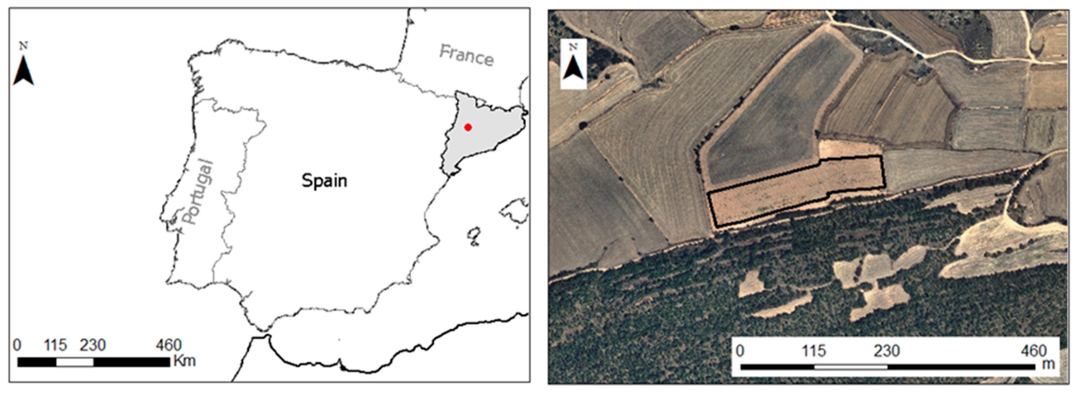
The experiment was located in Oliola, Lleida, NE Spain (Figure 1). Coordinates are 41°52”30’ N, 0°09”11’ E with altitude of 440 m above sea level. The experimental site is flat and open. The soil is deep (>1 m), non-saline and calcareous, classified as Typic Xerofluvent [27] with a silty loam texture, an average organic carbon content of 11.67 g kg−1, calcium carbonate content of 300 g kg−1, and pH of 8.2 (1:2.5 soil: distilled water).
A detailed study on soil physical characterization and instrumentation was performed in a plot representative of the area. The experimental field had a four year rotation which included wheat (Triticum aestivum) and barley (Hordeum vulgare) maintained during one and three years, respectively, as the main crops. Fallow years were also present. Usually, the crops were sown in late October and harvested at the end of June–early July.
2.2. Climate Conditions
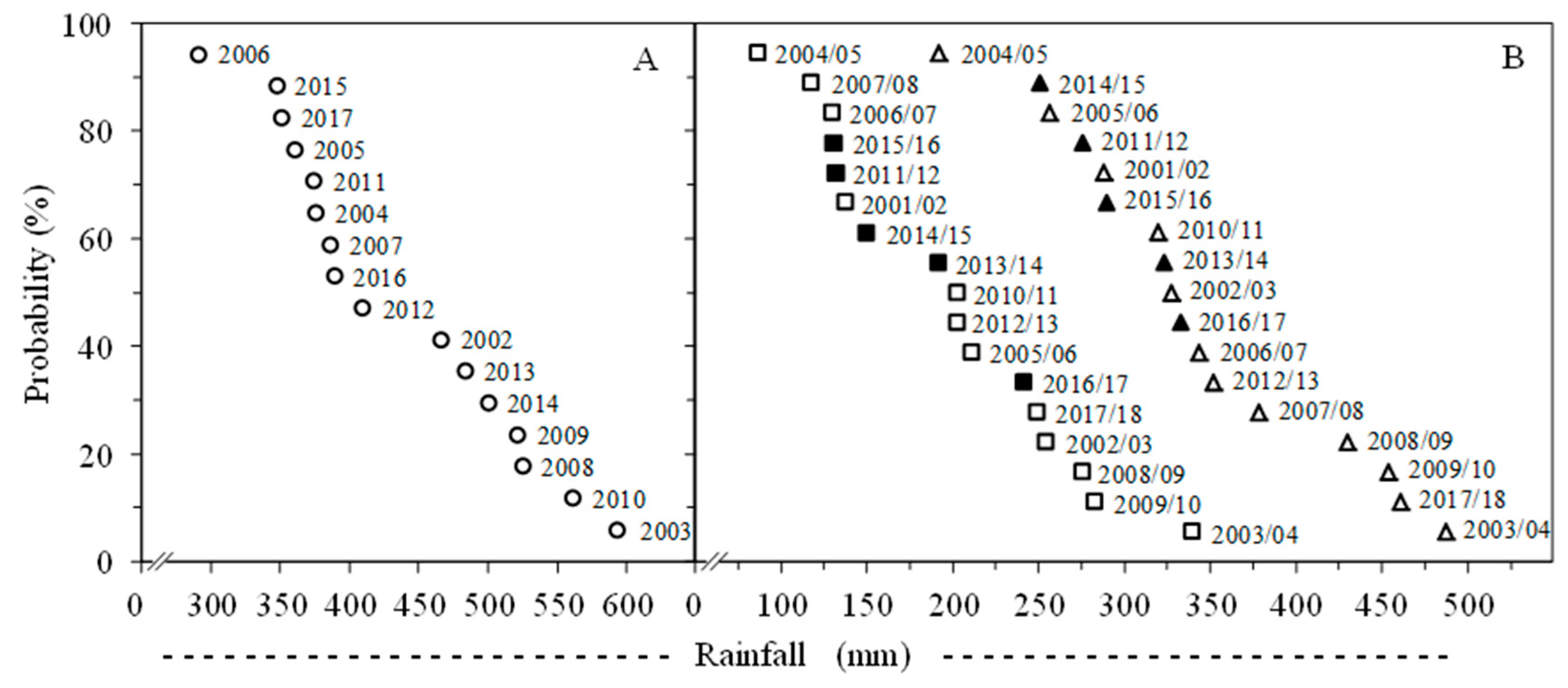
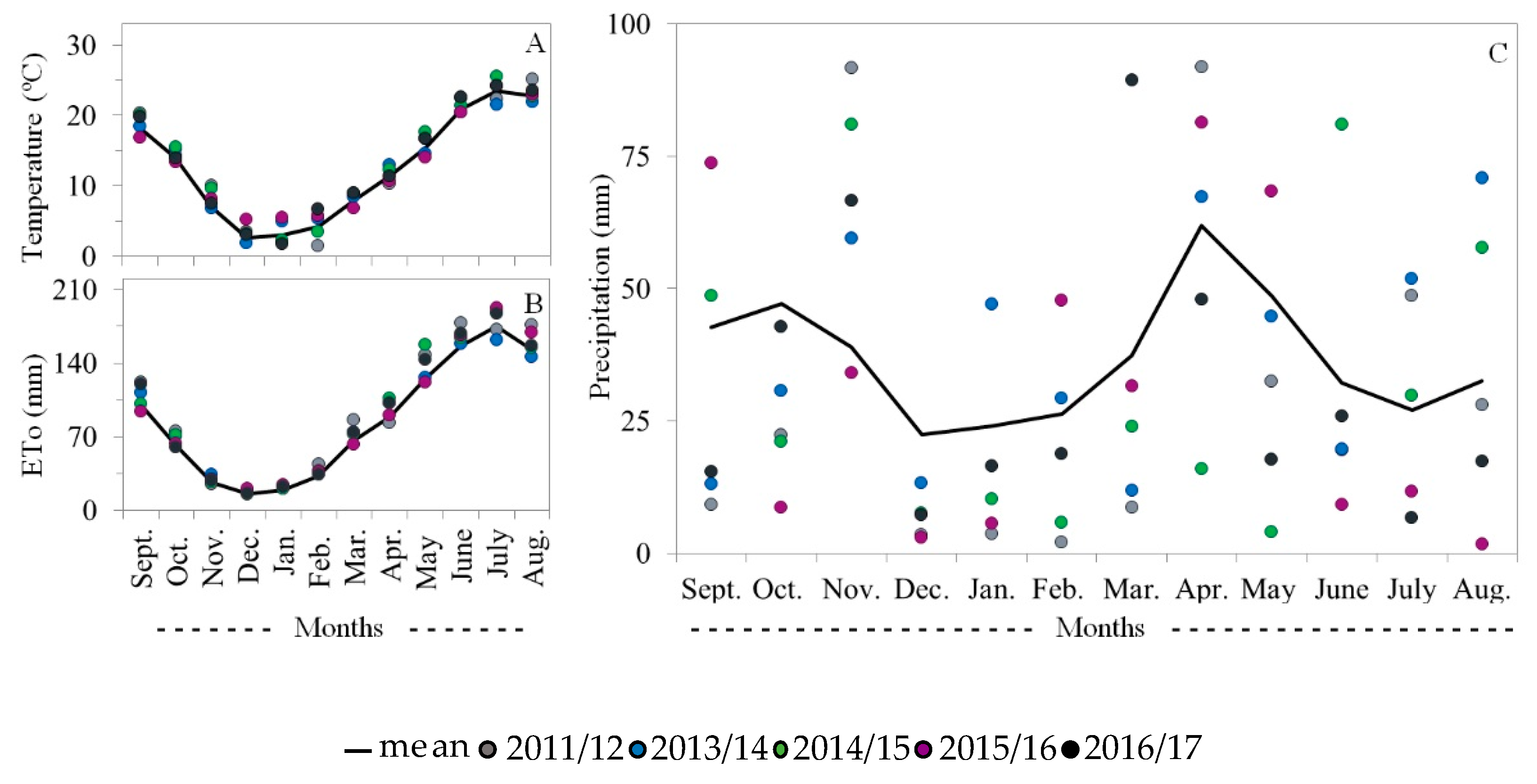
The area has a semiarid Mediterranean climate with a mean annual temperature of 12.6 °C with a maximum monthly average of 19.8 °C in August and a minimum monthly average of 5.8 °C in January. Daily meteorological data, precipitation, air temperature and evapotranspiration were obtained from an automatic station next to the field. The mean annual precipitation was 443 mm, and ranged from 291 mm to 593 mm (years 2006 and 2003, respectively) for the period 2002–2017. Within the year, maximum monthly precipitation occurs in April, followed by October and November. The probability of cumulative precipitation for the mentioned period indicates that for half of the years, annual precipitation was 390 mm or lower and in 25% of the years the cumulative precipitation exceeded 500 mm (Figure 2A). During the crop cycle, less than 350 mm of water are available to plants. This amount can be reduced to less than 190 mm (Figure 2B).
Extreme events range between 60 and 100 mm in a 100-year return period (Table 1). Rainfall data come from the local estimation proposed by Santamaría [28] and they were compared against the proposed rainfall values from Casas [29]. These data were considered in order to detect maximum potential leaching.
2.3. Soil Properties
Soil physical and chemical characteristics are shown in Table 2. Two main horizons were described from 0 to 32 cm and from 32 to 138 cm. The soil profile was divided into three depths, 0–30, 30–60 and 60–90 cm. The second horizon was divided in two for soil water records because root winter cereal density between 30–60 cm (data not shown) is higher than between 60–90 cm [30]; the later was considered the limit for cereal rooting depth in the area.
Soil texture was obtained from the particle size analysis (Pipette method, [31]). Organic carbon was assessed with the Walkey-Black method [32]. Soil bulk density (ρb) was determined from the soil dry weight of a known soil volume sample (100 cm3) and the average value of each layer was calculated (n = 4). Saturated hydraulic conductivity (Ks) and infiltration velocity were obtained from field measurements in the experimental plot with the Guelph permeameter (model 2825KI, Soil Moisture Equipment Corp.), and with a tension infiltrometer (model 2826D20, Soil Moisture Equipment Corp.), respectively. The soil water retention was determined in the two upper layers using the pressure plate apparatus at different matric potentials ψ (kPa). At the higher matric potentials (−33 and −100 kPa) it was done in disturbed and undisturbed soil samples to identify differences associated to the soil structure or potential compaction.
2.4. Data Acquisition
Soil water content data was obtained from 2011/12, 2013/14, 2014/15, 2015/16 and 2016/17 cropping seasons although the field was maintained under fallow in 2013/14 and 2016/17 (Figure 3).
Data came from two sources: by means of frequency domain reflectometry probes (ECH2O soil moisture probes, Decagon Devices, Pullman, Washington, USA, 2002); hereafter, it will be referred as “ECH2O” sensors, and by disturbed soil samples (DISSA). The ECH2O sensors are devices that measure volumetric water content via the dielectric constant of the soil using capacitance technology [33]. In 2006, the ECH2O sensors were installed at six points of the experimental field in the four soil layers (0–30, 30–60, 60–90 and 90–120 cm) and calibrated using field soil water measurements obtained weekly during three months (data not shown). One of them was located in the plot where the soil characterization was carried out. Daily SWC was automatically recorded at four-hour intervals and converted on a daily basis, since then. The output signals of the probes were transformed according to the manufacturer’s advice to obtain volumetric SWC values for each layer.
From the beginning of the experiment, SWC was monitored at three depths (0–30, 30–60 and 60–90 cm) from disturbed soil samples. Soil samples were collected periodically throughout the crop cycle. Samplings were made with a soil auger close to the ECH2O sensors. In each sampling date, between 3–6 soil samples were taken in different points of the experimental site. Gravimetric SWC was determined by oven drying 20 g of disturbed soil sample at 105 °C until constant weight. Then, the volumetric water content (θv) was calculated multiplying gravimetric water content (θg) by the ρb. Soil water storage (mm) was calculated by multiplying θv for the thickness of the soil layer. Finally, total water content was obtained from the sum of the partial water content of the three layers.
Samplings were done before sowing, at cereal tillering and after crop harvest. During the 2011/12, 2013/14, 2014/15, 2015/16 and 2016/17 cropping seasons, soil samples were taken before sowing (September or October) and in the following month: at cereal tillering stage (late January, early February), at spring time (between March–May) and after crop harvest (June).
Soil water dynamics were evaluated with the LEACHM model. Two cropping seasons under fallow (2013/14 and 2016/17) were included in the study. Barley was cropped in the 2011/12, 2014/15 and 2015/16 seasons, which were used in the evaluation. The later cropping seasons covered the rainfall variability (Figure 4) and yield variability (from 5 to 8 Mg ha−1).
Soil water content from DISSA provided more precise measurements, but daily records were lacking. Thus, for daily records, ECH2O sensor data were used. Soil water content values from midday were chosen and data were taken from 2011 onwards. Data were obtained for the five years from the sensors’ installation, meaning that there was enough time to obtain a robust SWC data set. Before the model evaluations, ECH2O sensor data were compared against DISSA data using linear regressions to decide the time period to be used in the LEACHM model.
2.5. LEACHM Model
As our dryland agricultural system is characterized by transient water fluxes, the water module belonging to the LEACHM model was used to evaluate the water drainage below 90 cm and the water balance in the soil profile. It is considered a vertical unidimensional mesh, which is divided into an equal number of horizontal layers, and time is split into intervals shorter than a day. This model describes the one-dimensional water flow in the unsaturated zone using the diffusivity form of the Richards’ equation, solved by the Crank and Nicolson method [34]. For this, it is necessary to know the relations between hydraulic conductivity, volumetric moisture and matric potential. Those are based on the moisture retention function (Equation (1)) and the unsaturated hydraulic conductivity function (Equation (2)) proposed by Campbell [35]:
where h is the matric potential, a is the air entry water potential and b is an empirically determined constant, θs is the volumetric water content at saturation, Ks is the saturated hydraulic conductivity and p is an interaction parameter about pore size, the value of which is assumed to be 1 for the LEACHM model. In addition, LEACHM uses the wet-end modification of Hutson and Cass [36] which introduced a sigmoidal function without discontinuities. The calculated θs value from 0 to 30 cm coincided with our field measurements (Table 2). A free-draining lower boundary was assumed because no plough layers or equivalent limiting drainage, have been described in this plot.
Weekly potential evapotranspiration (crop reference evapotranspiration ET0, obtained with Penman-Monteith equation [37]) was introduced in the input data file of the LEACHM model. Daily potential evapotranspiration (ET) is calculated as one-seventh of the weekly potential ET. The LEACHM model uses the crop cover fraction to separate potential ET into potential evaporation and potential transpiration. Potential ET for a time step is calculated following Childs and Hanks [38]. It was also assumed that both evaporation and transpiration start at 0.3 day (7h 12) and they end 12 h later (0.8 day). A sinusoidal variation of potential ET flux density (mm day−1) was included with the final aim to calculate the fraction of total ET lost during a determined time interval. The potential evaporation and the maximum evaporative flux density were considered to calculate the actual evaporation. The plant water uptake at z depth and a time interval t was calculated following Nimah and Hanks [39] as:
where U(z,t) is the transpiration sink term in the Richards equation (day−1), Hroot is the water potential at the root-soil interface (mm), z is depth (mm), (Rc + 1) is a root resistance term (mm), h(t) is the soil water pressure head (mm), s(t) is the osmotic potential (mm), RDF is the fraction of total active roots in the soil layer, K(θ,t) is hydraulic conductivity (mm day−1) for soil water content θ and Δx is the conceptual distance from the point where h and s are calculated to the plant root (fixed at 10 mm in the code). Richard’s equation is solved for each soil layer an each flow interval with a periodicity of 0.05 day or less depending on the water flow. The model requires input data about soil physical properties, water inputs (rain events), weather and crop data. Soil physical properties, such as texture, organic carbon, ρb, water retention curve and Ks at the three soil layers, were selected from Table 2. Daily accumulated rainfall figures were the water inputs and were taken from the meteorological station. Meteorological data were the weekly values of potential evapotranspiration, mean temperatures and thermal amplitude. They were calculated from the daily data sets. Finally, crop data referring to plant characteristics (planting, emergence, plant and root maturity, crop cover fraction at maturity, harvest dates), crop growth (crop cover fraction) and fertilizer applications were obtained from the experiment’s field observations.
2.6. Model Calibration and Validation
The approach for evaluating water dynamics with the LEACHM model was from the simple case study (fallow period) to a more complex assessment (cropping period). The selected simulation periods were chosen to account for the lowest and the highest SWC data linked to a driest cropping season and a rainy period (under fallow). Soil water dynamics using DISSA were evaluated for the whole crop cycle. The starting simulation day was selected according to the first sampling day, related to the sowing time. The end day was considered to be a week after the last sampling day at harvest. Only for the fallow year 2013/14, a longer period was considered: from September 2013 until October 2014, when barley was sown. Meanwhile, soil water dynamics using ECH2O sensor data were evaluated for a six-month period from 1st October to 31th March of each cropping season. No longer period was selected because under dry summer conditions of the experimental site (Figure 4) ECH2O sensors do not work properly because the pores have not a required minimum water content. During the 2015/16 crop year, data entry from the ECH2O sensors stopped for part of the time; thus, only 119 d of SWC were recorded. Selected ECH2O data were adjusted according to the field moisture data, as they were obtained from independent devices located in the soil at different depths. Once data were collected and properly organized, LEACHM model evaluation was performed (Figure 3). It consisted in calibration and evaluation. First, two fallow seasons were calibrated-validated and then, plants were introduced with three barley cropping seasons. In both cases, observed and modeled SWC data were compared.
Sensitivity analysis evaluates the effect of different parameters on the modeling of the volumetric SWC with the LEACHM model [21,40,41]. Sánchez-de-Óleo [21] found that the most highly influencing parameter was the b coefficient of the Campbell equation, and he gave less importance to the a coefficient of the equation. According to this author, the saturated hydraulic conductivity was not a sensitive parameter. Calibration was performed by running LEACHM with two data sets, the 2013/14 period for fallowing and the 2015/16 period for cropping land use (Figure 3). An optimization procedure based in the Nelder-Mead simplex method was used to adjust the parameters of the Campbell equation [42]. This is a direct search method that does not use numerical or analytic gradients and minimize an objective function in a multidimensional space according to values of the function. The measured SWC values for each land use and data origin was used for calibration (Figure 3). A range in the coefficient values and an initial input value for each coefficient were needed. To calibrate the b coefficient, it ranged from 3 to 15 in the upper layer and from 5 to 15 in the other two deeper layers. The a coefficient calibration values ranged from −5 to −2 kPa only for the upper layer. The variation ranges chosen for parameters a and b were similar to those used in other calibrations of the LEACHM model [21,41]. The second and the third layer were manually adjusted, according to the a upper coefficient. Calibration was finished when the a and b adjusted parameters did not significantly change after the iterations. At that point, the error differences between observed and simulated SWC in profile were minimized.
Five statistical parameters were used to evaluate the model. The mean difference (MD) and the determination coefficient (R2) criteria served to compare model predictions between observed (Oi) and simulated (Si) values:
where Ō and are the average of the observed and simulated values, respectively. Additionally, other statistical parameters were used. The root mean square error (RMSE) evaluated the differences between observed and simulated SWC, the normalized root mean square error (NRMSE) set the differences and compared differences between years, and the agreement index (d) evaluated the model fitting [21,43]:
Validation was done by running LEACHM with three different data sets, 2016/17 for fallow land and 2011/12 and 2015/16 for cropping land use (Figure 3). The a and b coefficient values obtained from the calibration were maintained for validation in the following seasons. Drainage and volumetric SWC for each layer were obtained from the model. Observed and simulated values were also evaluated as mentioned above.
The water balance components we used were the soil water storage, the initial and final soil water depth, rainfall, evaporation (fallow periods) evapotranspiration (cropping periods) and drainage. They were calculated for all the evaluated years. These terms were obtained from the simulations performed with the calibrated model using ECH2O sensor data.
3. Results
3.1. Parameters Calibration
Initial and calibrated coefficient values are shown in Table 3. The range of variation of the calibrated parameter a was lower under fallow conditions than with the barley crop (−4.95–−5.00 kPa and −2.00–−3.00 kPa, respectively). The most pronounced change corresponded to parameter b in fallow conditions (6.08–9.87) than under cropping (6.63–8.81). The highest values of b correspond to the calibration made with the data set of soil moisture obtained by soil sampling. However, the values obtained using the ECH2O data set provide a characteristic curve for the soil very similar to that obtained with the pressure plates (Table 2).
In the fallow period, the calibration increased the value of parameter b and decreased the parameter a in the upper layer with respect to the initial values, regardless of the data origin. In the deeper soil layers, the values of b decreased and those of the parameter a slightly increased. In the crop cycle, the calibration supposes, in all cases, a reduction of the parameter a with respect to the initial values, while the parameter b increased in the superficial layer and decreased in the other two layers. The calibration led to similar a values in the three layers, and a b value staggering, corresponding the highest value to the surface layer.
Hydraulic parameters calibration of the model when plants were established resulted in higher values of the parameter b in the three layers of the soil profile when the ECH2O data set was used, with a smaller error in the adjustment to the measured data.
3.2. Soil Water Content Modelling in a Fallowing Period
Statistical parameters from the soil under fallow showed a better data adjustment for the calibration than the validation cycle (Table 4). A general overestimation of the SWC was found, except for the 30–60 cm soil layer. Differences in the total SWC ranged between 11 and 25 mm of water according to the RMSE (Table 4). A good match between observed and simulated data was confirmed with the NRMSE (<0.3) and the agreement index (>0.5) in most of the cases. The biggest differences in NRMSE were observed in the upper layer, except for the deepest layers with ECH2O sensor data. For the soil profile, the error ranged between 5% and 14%, corresponding to the lowest NRMSE values of the calibration period.
Finally, when the ECH2O data set was used, d coefficient was higher for the calibrated than for the validated fallow cycle; however, when using soil sampling data, this coefficient was higher for the validation period. In the fallowing seasons the model explained the variability of observed data, with some exceptions mainly in one layer (60–90 cm) during the 2013/14. Aside from those low values, the R2 from modeling with the DISSA data set doubled the values from the modeling with the ECH2O sensor data.
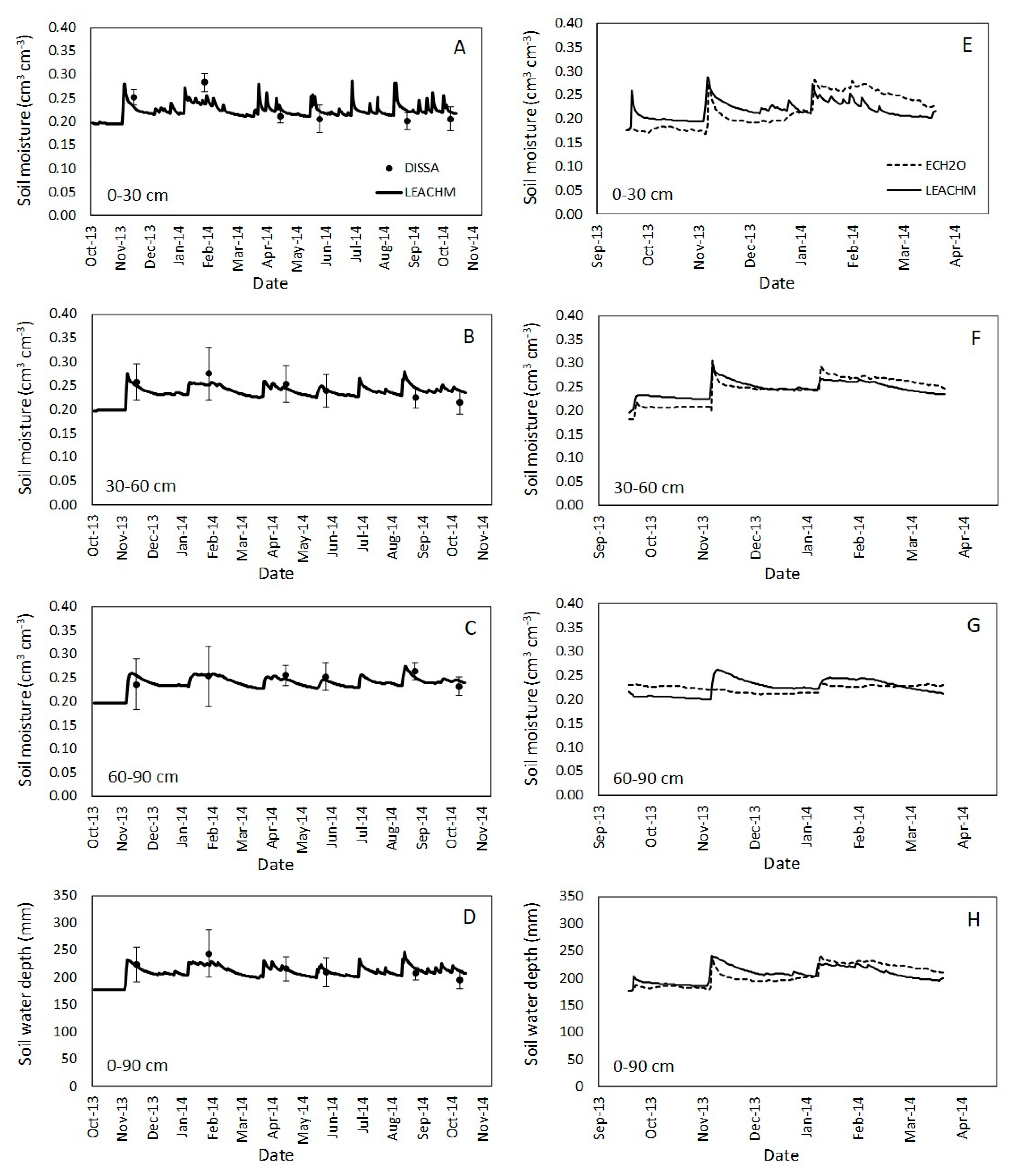
Graphical evaluation showed differences in the calibration (Figure 5) and the validation seasons (Figure 6), using both data sets. Soil water dynamics were higher in the upper layer and decreased with depth over time. The SWC was better simulated during the calibration than the validation seasons. Both data sets were independently calibrated but similar simulated SWC was observed in the calibration season (Figure 5). On the contrary, the validation season showed considerable differences between observed and simulated SWC (Figure 6).
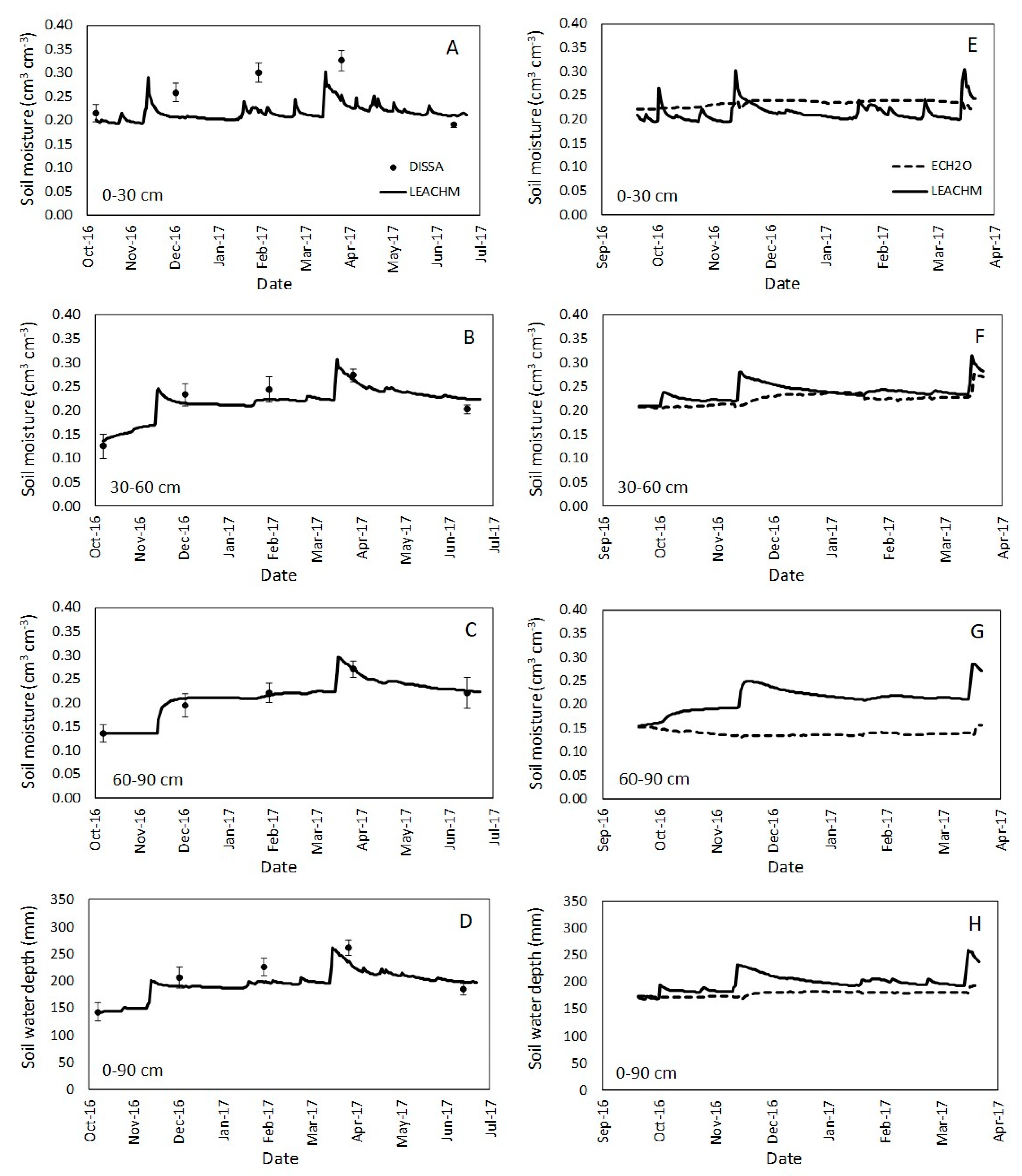
The main differences between measured and simulated SWC occurred in the superficial layer of soil during the validation period (Figure 6). The LEACHM model underestimated the moisture values in the upper layer measured with both sets of SWC input data. The values recorded by the soil moisture probes in the three soil layers during 2016/17 season were anomalous, as they hardly changed over time. Therefore, the dynamics of water in the soil did not reproduce well, since there was almost no response to water inputs in the soil profile due to rain. In the fallow periods, SWC values at the end of the period (June) are of the order of 0.20 cm3 cm−3, while the highest values are 0.30 cm3 cm−3, regardless of the soil layer considered. This range of soil moisture was similar in the three layers, confirming the homogeneity of the soil profile in this area.
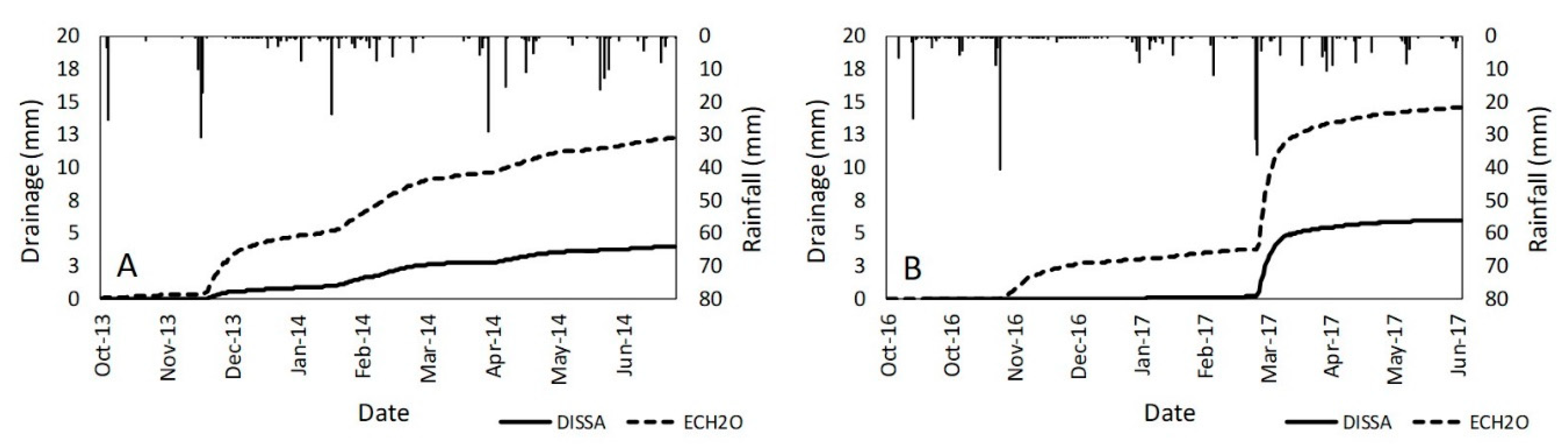
Cumulative drainage at 90 cm was related to the rainfall events (Figure 7). The 2013/14 season displayed a continuous increase in the drainage over time, while the 2016/17 season followed a sigmoidal function. Changes in water losses increased when rainfall was higher than 20 mm, and these precipitation events generally occurred in autumn and early spring. Drainage below the root zone (>90 cm depth) was from 3.0 to 14.5 mm. Considerable differences were obtained from the LEACHM evaluation respect to the dataset type used. Simulations made with ECH2O calibration displayed drainage values which were three times greater than those obtained with DISSA calibration. These differences are due to the different values of parameter b obtained with each data set. The higher values provided by the calibration with DISSA resulted in a higher water retention capacity of the soil and, therefore, a lower drainage.
3.3. SWC Modelling in a Barley Crop Soil
Statistical parameters of SWC simulations showed that LEACHM modelling in barley cropping seasons (Table 5) did not fit as well as in the fallow seasons (Table 4). The R2 results were considerably lower than those obtained during the fallow seasons. The smallest values were obtained from modeling with ECH2O data for the calibration period. There was a general SWC underestimation in the upper soil layer and in the total SWC. Soil water modeling using the ECH2O data set showed better adjustment than those made with DISSA, although the agreement index was similar in all cases regarding to the soil profile. Mean differences between observed and simulated water depth varied from 1 to 20 mm, and were supported by the NRMSE results, which ranged from 0.04 to 0.25 for water depth at 0–90 cm.
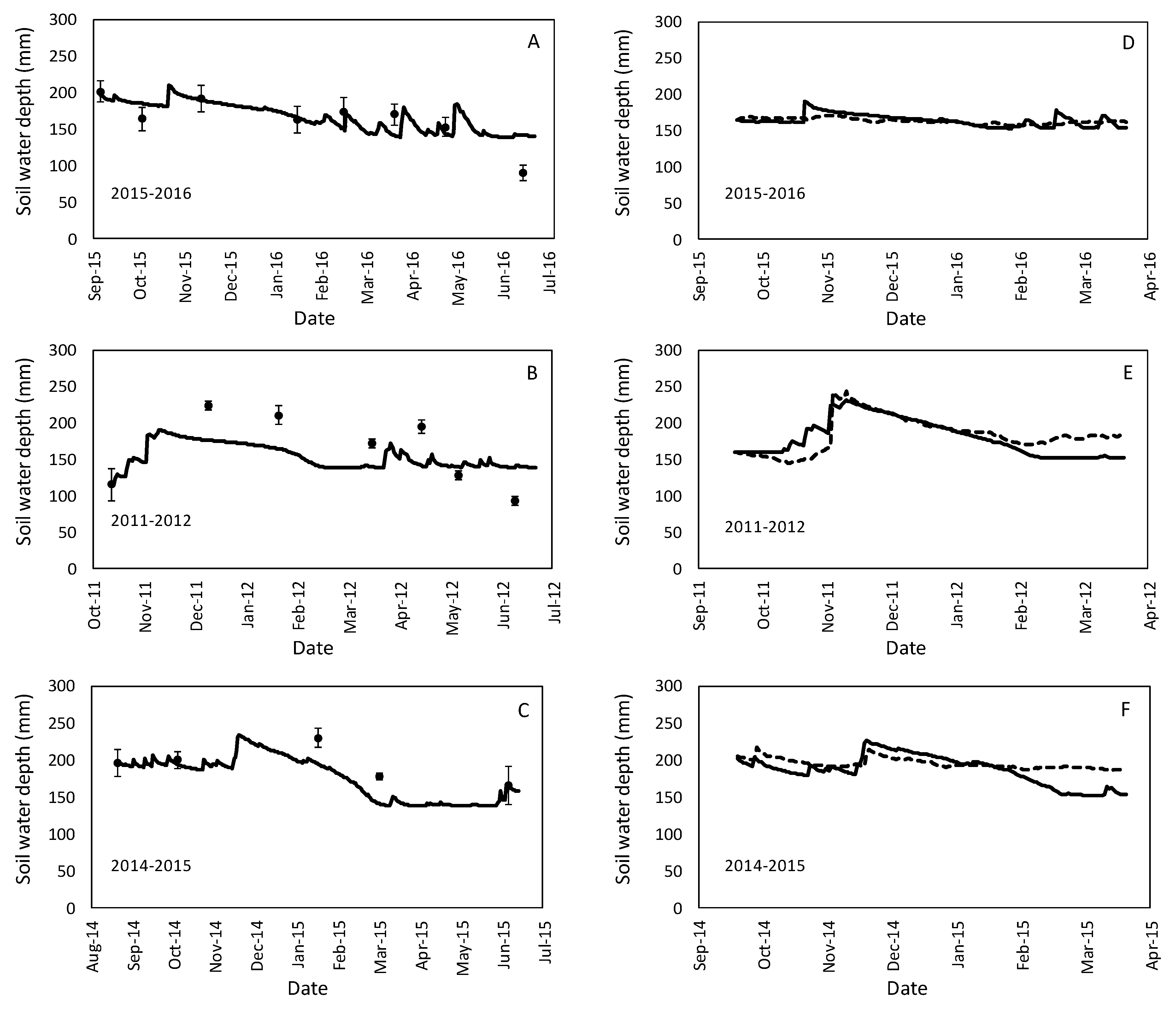
Crop seasons calibration fitted better than validation over time (Figure 8). LEACHM overestimated water content predictions at the end of the 2011/12 season: they were 95% higher than the values obtained from DISSA samples. A similar result occurred at the end of the period 2015/16. When the LEACHM model was run with the DISSA data set, it was observed a SWC under and overestimation at the wettest and driest periods of the cropping season. The last of these coincided with the summer period when evapotranspiration was the highest (Figure 2). The rainfall effect on the SWC evolution over time was marked in the simulations performed with DISSA dataset. Measured SWC with the ECH2O sensor did not detect important changes over time, limiting the accuracy of the LEACHM simulations. The best fit was observed during the wettest period but differences among simulated and observed values increased up to the end of the validation period.
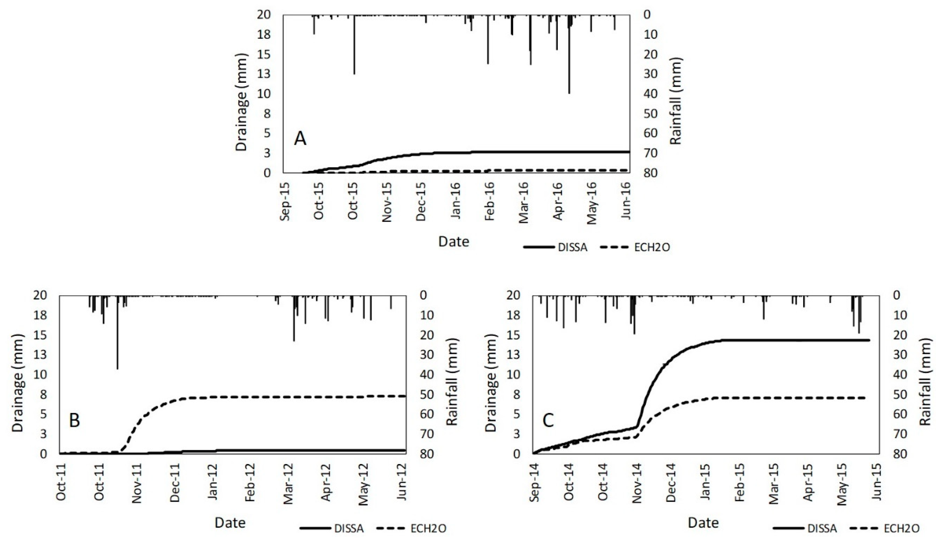
The accumulated drainage predictions with barley varied according to the dataset used for the calibration (Figure 9). Cumulative drainage followed a sigmoidal function and ranged between 0.3 and 14.3 mm of water (2015/16 and the 2014/15 seasons, respectively). The barley crop cycles received on average 20% less rainfall than the fallow cycles (Figure 7 and Figure 9), which together with the presence of plants resulted in less drainage. In two out of three evaluated cropping seasons, the highest water losses were obtained from the simulation with DISSA data, probably as a consequence of the lower retention capacity obtained with DISSA data set in the barley season. The water losses were observed during the first 100 days, which corresponded to the period between sowing and cereal tillering but also coincided with a marked precipitation period. After that, soil water drainage reached a plateau up to the end of the crop cycle. Soil water content at the end of summer affects the drainage amount as it mainly occurs because of autumn rains. Rains of the same amount in the months of October and November can produce different drainage dynamics depending on the existing water content in the upper soil profile.
3.4. Water Balance
The water balance components from the simulations performed with the calibrated model using ECH2O data are shown in Table 6.
During the two years under fallowing, the soil increased its water content by around 20 mm, while in the periods with barley there was a decrease in the amount of water stored in the soil profile. The net water recharge represented 10% of the water content in the soil profile. Higher percentages (over 20%) were obtained when the calibrated model was used with the DISSA moisture data set (data not shown). Water drainage oscillated between 0.3–14.5 mm, representing less than 10% of the water in the soil and less than 5% of the rainfall.
4. Discussion
4.1. Soil Water Dynamics
Using the optimal parameters obtained in the rainfed system, the SWC predictions obtained for soil water depth are quite reasonable with both data sets for calibration taking into account that the driest periods were omitted for ECH2O sensors. Soil water dynamics simulations with LEACHM model fitted better in the fallow seasons (Table 4) than when crop season data were included (Table 5), according to the statistical evaluation. However, differences in water content estimation were lower than 25 and 15 mm for the crop and fallow seasons, respectively, indicating a good SWC estimation using LEACHM model in a dryland system.
Simulations under fallow fitted better as LEACHM uses simple relationships related to water demand (evapotranspiration) and plant growth. The increase of SWC by 20 mm of water recharge could be higher since the evaporation simulated by the model could be overestimated [26]. The soil tillage carried out during the fallow cycle would break the pores continuity in the surface layer and decrease the evaporative flow from the deeper layers of the soil to the surface [44,45]. In fallow periods, the amount of rainfall mainly determines the recharge at the begin46ning of spring, since the simulated drainage in this period is similar to that of the periods with barley cultivation despite having greater precipitation (50 mm).
Predictions on soil water dynamics offered a global overview about how water moves through the soil profile, despite the R2 < 0.62 in crop barley simulations. During the growing periods, the water recharge is negative in the rainfed systems that have rainfall below 340 mm per year.
Soil characteristics played an important role in modeling. Texture and Ks are key parameters in the assessment of SWC and drainage, as the estimation of the a and b parameters depend on these variables. Texture would influence the underestimation of SWC in the 30–60 and 60–90 cm soil layers in this experiment, because of the silt content in both layers (49 and 60% respectively). Johnson et al. [46] reported that coarse fractions enhanced water movement through the soil profile, producing an overestimation in SWC from 45 to 75 cm depth, but an underestimation for the upper 30 cm in sandy-loam fallow plots. It must be pointed out that at the end of the growing season the soil moisture is below even the permanent wilting point. The barley crop seems to be adapted to these dryness levels. However, neither the ECH2O probes nor the LEACHM model are capable of reproducing these low values of soil moisture.
Data origin also affected LEACHM simulations. Soil water content obtained from DISSA adjusted better than those obtained from the ECH2O, mainly during the fallow seasons. Other authors pointed to more accurate predictions with the LEACHM model when the K-θ-ψ relationships derived from the in-situ measurements were used [23]. Moreover, the ECH2O probes did not easily detect changes in SWC over time as observed with DISSA samplings. The ECH2O probes are used for irrigated fields where water is usually kept above 50% of the water pore fill capacity. In rainfed systems, this condition was not achieved during the whole crop cycle because of the low precipitation amounts or the air temperature increases.
After prolonged dry periods, the lack of soil moisture would lead to a reduction of the contact area between the soil and the ECH2O sensor. In our case, there was no response from the sensors to the rains during the autumn-winter period of the 2016–2017 years, but the increase of soil moisture, due to the rains of the following months, restored accurate measurements of the sensors (data not show). This process is not immediate, and it is very dependent on the season and the amount of rainfall recorded. The rewetting of the sensors after these periods of low rainfall is very slow and may be the cause of the lack of response that can be prolonged over time. Thus, the resonance frequency used by the sensors to calculate the dielectric constant would be wrongly measured and so would the volumetric water content. Similar findings were reported by Czarnomski et al. [11] who found that the ECH2O device underestimated the soil moisture when the temperature increased from 22 to 31 °C. They found a 1.9% data deviation, but the experiment was performed under controlled conditions, meaning that bigger differences in the field, such as ours, would be expected. This limitation of the ECH2O probes to measure SWC in very dry soil conditions reduces the goodness of the calibration process with this data set. A retroactive calibration of the humidity sensors may be necessary. Incorporating soil physical information using pedotransfer functions can be improve sensor accuracy, as established by Gasch et al. [47]; however, the lack of contact between the sensor and the soil can hardly be corrected by an adequate calibration. Additional data set of soil water content obtained from field measurements can be very useful to recalibrate these sensors. In addition, inverse calibration could be carry out using the adjusted model for obtain realistic measures of the sensors in prolonged dry periods.
The rainfall regime is very important for soil water dynamics. Heavy rains concentrated in the period of low crop coverage increased the recharge, compared to periods with little rainfall much more spread over time. Water moved through the soil profile following the precipitation events. Crop presence or absence showed differences in SWC variations along depth and over time. In fallow seasons, rainfall events promoted changes in SWC even at the deepest layer. On the contrary, in barley cropping seasons, the upper layer was the most prone to SWC changes, due to the direct soil contact with the atmosphere (rainfall, wind, solar exposure). In the second layer, the soil system interacted with plant roots and living organisms, reducing the variations in SWC. Finally, in the third layer, the soil system had few interactions with the barley roots and the atmosphere, leading to a stable soil system with few fluctuations in water content over time.
Land use resulted in a total water gain or lost at the end of the crop cycle. The fallow period was a recharge period because soil gained water at the end of the season. After the barley crop, SWC diminished as plants took water from the soil for their growth. Moret et al. [6] reported similar results in another dryland Mediterranean environment with lower mean precipitation than this site. In dryland environments with erratic rainfall distribution, such as this experimental site (Figure 4), fallow increased the available water for the next cropping season. Thus, it would reduce the risk of plant mortality in case of drought at sowing time and an increase in grain yield compared with a continuous cropping system [6].
4.2. Drainage Modelling
Drainage estimate with the LEACHM model is acceptable as the model explains the SWC in profile satisfactorily. Rainfall (amount and distribution) and land use drove the volume of water loss over time. Effective rainfall can be considered lower than 20 mm as drainage was mostly produced above this precipitation value.
Cumulative drainage was higher at fallow than at barley cropping seasons, as there were no plants to take water for growth in the first scenario. Average precipitation in fallow years was higher than for the barley crops. However, only in the 2016/17 fallow season precipitation was above the mean values for the area (Figure 2) probably related to the previous dry and warm summer season (Figure 7). According to probability figures, the results mean that at least one out of two seasons, the system can lose 5.9 mm of water per fallow period.
In the 2014/15 season, drainage was considerably higher than all the other years. A marked increase in water losses was registered during a two-month period (December 2014 and January 2015) which recorded 33 days with rainfall. In 29 of them, daily precipitation was <1 mm (Figure 9). Consecutive precipitation values <1 mm would lead into a problem calculation in the LEACHM.
Maximum water losses were observed at the beginning of the season, from sowing until cereal tillering stage, because it is a period with no plants or when they are not large enough to use the water entering into the soil system. It also coincides with a high precipitation amount period and with the two most common N applications. Considering the return period of the precipitation, there is a probability between 60–70% of drainage from 6.1–7.2 mm of water during the winter season, the most prone to leach NO3−-N to the groundwater. The results alert about drainage in dryland agriculture systems and the potential associated impacts, contrary to the premised by other authors [48]. This scenario reinforces the importance of our results for environmental impacts over underground waters by solutes than can be leached.
Minimal or zero water loss values were obtained from cereal tillering until the end of the season. Lack of drainage can be explained by meteorological and agronomic reasons. After cereal tillering, plants increase their water consumption. From spring onwards, temperatures started to rise as well as evapotranspiration.
Compared to other rainfed environments, estimated drainage values (<15 mm) can be considered as small water losses [23,49]. Data accuracy is a key factor in model calibration [12] but data are difficult to obtain due to the soil heterogeneity, porous complexity, water spatial and temporal water dynamics [9]. Without drainage field measurements, appropriate SWC monitoring would lead to proper drainage estimation. The ECH2O probes were easily managed devices, which would be monitored and corrected with periodical field measurements over time and along soil depth but their use is limited over the year in semiarid environments.
In general, the losses during the fallow years were higher, coinciding with the greater amounts of drainage, showing the importance of the water balance as an indicator of the leaching potential of the system.
Despite the finding that estimated drainage is small and the potential for leaching is also low, it is necessary to maintain adequate agronomic practices such as fertilization guidelines in these areas to prevent the NO3−-N accumulation in the soil profile. The maximum 24-h precipitation in the set of years considered corresponded to the period 2016/17 was 41 mm, while the drainage for this period was 14.5 mm. However, for a return period of 25 and 50 years, the maximum expected precipitation is 70 and 90 mm, respectively (Table 1). The simulations carried out, replacing the 41 mm rainfall by these predicted values, would cause an increase in the drainage of between 2.1 and 3.3 times that obtained with the current maximum 24-h value. These figures are meaningful in a context of climate change, in which forecasts in the Mediterranean area indicate that short but heavy rainfalls are liable to increase in number [4,50]. Thus higher amounts of drainage could occur, which would increase the risk of groundwater contamination in a huge vast world area [5].
5. Conclusions
The LEACHM is a robust model to simulate soil water dynamics in a fallow period in the 0–90 cm depth in a semiarid rainfed agricultural system. As crops were introduced, LEACHM lost accuracy in predicting SWC at the different layers, but an acceptable overview of the soil water was obtained and can be used for environmental purposes linked to drainage. Fallow periods resulted in a little soil water recharge, which did not occur in years with barley cultivation. Drainage losses in this system are small (<20 mm) and usually occur in the autumn-winter period. Under these conditions, the potential impact of water solutes on underground water will be mainly related to their concentration in soil-water solution. Field soil moisture measurements could be more realistic than capacitive sensors when feeding data into models in dryland systems due to the lack of response after prolonged dry periods.
Author Contributions
Proposal, À.D.B.-S. and A.L.; Data acquisition, À.D.B.-S. and D.E.J.-d.-S.; Conceptualization, D.E.J.-d.-S., A.L. and À.D.B.-S.; Methodology, D.E.J.-d.-S. and A.L.; Writing-Original Draft Preparation, D.E.J.-d.-S.; Writing-Review & Editing, A.L., À.D.B.-S. and D.E.J.-d.-S.
Funding
This research was funded by the Spanish Ministry of Economy and Competitiveness and the Spanish National Institute for Agricultural Research and Experimentation (MINECO-INIA) through the projects [RTA2013-57-C5-5] and [RTA2017-88-C3-3]. The PhD studies of D.E. Jiménez-de-Santiago were funded by the JADE-Plus scholarship from Bank of Santander-University of Lleida.
Acknowledgments
The authors would like to thank the anonymous referees for their suggestions and comments. J. Llop and S. Martínez are fully acknowledged for their field assistance and M.F. Mor, J.C. Balasch and D. Ginestar for cabinet assistance.
Conflicts of Interest
The authors declare no conflict of interest.
References
- European Union. Council Directive 91/676/EEC, of 12 December 1991, concerning the protection of waters against pollution caused by nitrates from agricultural sources. Off. J. Eur. Communities 1991, L375/1–L375/8. [Google Scholar]
- Mateo-Sagasta, J.; Marjani, S.; Turral, H. (Eds.) More People, More Food, Worse Water? A Global Review of Water Pollution from Agriculture; Food and Agriculture Organization of the United Nations (FAO): Rome, Italy; International Water Management Institute (IWMI): Colombo, Sri Lanka, 2018; ISBN 978-92-5-130729-8. [Google Scholar]
- Sordo-Ward, A.; Granados, I.; Iglesias, A.; Garrote, L. Blue Water in Europe: Estimates of current and future availability and analysis of uncertainty. Water 2019, 11, 420. [Google Scholar] [CrossRef]
- Rockström, J.; Karlberg, L.; Wani, S.P.; Barron, J.; Hatibu, N.; Oweis, T.; Bruggeman, A.; Farahani, J.; Qiang, Z. Managing water in rainfed agriculture—The need for a paradigm shift. Agric. Water Manag. 2010, 97, 543–550. [Google Scholar] [CrossRef]
- Ministerio de Medio Ambiente y Medio Rural y Marino (MARM). National summary of area, yield and production, 2015. In Statistical Yearbook; NIPO 013-17-118-2; MARM: Madrid, Spain, 2017; p. 791. (In Spanish) [Google Scholar]
- Moret, D.; Arrúe, J.L.; López, M.V.; Gracia, R. Winter barley performance under different cropping and tillage systems in semiarid Aragon (NE Spain). Eur. J. Agron. 2007, 26, 54–63. [Google Scholar] [CrossRef]
- Meco, R.; Moreno, M.; Lacasta, C. Productividad de sistemas de secano semiárido en manejo ecológico. In La Reposición de la Fertilidad en los Sistemas Agrarios Tradicionales; Garrabou, R., González de Molina, M., Eds.; Icaria Editorial S.A.: Barcelona, Spain, 2010; pp. 85–108. ISBN 978-84-9888-215-5. [Google Scholar]
- Robinson, D.A.; Campbell, C.S.; Hopmans, J.W.; Hornbuckle, B.K.; Jones, S.B.; Knight, R.; Ogden, F.; Selker, J.; Wendroth, O. Soil moisture measurement for ecological and hydrological watershed-scale observatories: A review. Vadose Zone J. 2008, 7, 358–389. [Google Scholar] [CrossRef]
- Shukla, M.K. Soil Physics: An Introduction, 1st ed.; CRC Press: Boca Raton, FL, USA, 2013; pp. 119–156. ISBN 978-1-4398-8842-1. [Google Scholar]
- Gardner, C.M.K.; Robinson, D.; Blyth, K.; Cooper, J.D. Soil Water Content. In Soil and Environmental Analysis, 2nd ed.; Smith, K.A., Mullins, C.E., Eds.; Marcel Dekker Inc.: New York, NY, USA, 2000; pp. 1–84. ISBN 0-203-90860-0. [Google Scholar]
- Czarnomski, N.M.; Moore, G.W.; Pypker, T.G.; Licata, J.; Bond, B.J. Precision and accuracy of three alternative instruments for measuring soil water content in two forest soils of the Pacific Northwest. Can. J. For. Res. 2005, 35, 1867–1876. [Google Scholar] [CrossRef]
- Lidón, A.; Ramos, C.; Rodrigo, A. Comparison of drainage estimation methods in irrigated citrus orchards. Irrig. Sci. 1999, 19, 25–36. [Google Scholar] [CrossRef]
- Jakubínský, J.; Pechanec, V.; Procházka, J.; Cudlín, P. Modelling of Soil Erosion and Accumulation in an Agricultural Landscape—A Comparison of Selected Approaches Applied at the Small Stream Basin Level in the Czech Republic. Water 2019, 11, 404. [Google Scholar] [CrossRef]
- Hutson, J.L. LEACHM, Leaching Estimation and Chemistry Model. Model Description and User’s Guide. School of Chemistry, Physics and Earth Sciences, The Flinders University of South Australia: Adelaide, Australia, 2003. [Google Scholar]
- Marinov, I.; Marinov, A.M.A. Coupled mathematical model to predict the influence of nitrogen fertilization on crop, soil and groundwater quality. Water Resour. Manag. 2014, 28, 5231–5246. [Google Scholar] [CrossRef]
- Porter, J.R. AFRCWHEAT2: A model of the growth and development of wheat incorporating responses to water and nitrogen. Eur. J. Agron. 1993, 2, 69–82. [Google Scholar] [CrossRef]
- Addiscott, T.M.; Wagenet, R.J. Concepts of solute leaching in soils: A review of modelling approaches. Eur. J. Soil Sci. 1985, 36, 411–424. [Google Scholar] [CrossRef]
- Bastiaanssen, W.G.M.; Allen, R.G.; Droogers, P.; D’Urso, G.; Steduto, P. Twenty-five years modeling irrigated and drained soils: State of the art. Agric. Water. Manag. 2007, 92, 111–125. [Google Scholar] [CrossRef]
- Greenwood, D.J.; Zhang, K.; Hilton, H.W.; Thompson, A.J. Opportunities for improving irrigation efficiency with quantitative models, soil water sensors and wireless technology. J. Agric. Sci. 2010, 148, 1–16. [Google Scholar] [CrossRef]
- Hutson, J.L.; Wagenet, R.J. Simulating nitrogen dynamics in soils using a deterministic model. Soil Use Manag. 1991, 7, 74–78. [Google Scholar] [CrossRef]
- Sánchez de Óleo, C.M. Estimación de Parámetros en Modelos de Transporte de agua y Nitrógeno en el Suelo. Ph.D. Thesis, Technical University of Valencia, Valencia, Spain, 2015. [Google Scholar]
- Ramos, C.; Carbonell, E.A. Nitrate leaching and soil-moisture prediction with the LEACHM model. Fertil. Res. 1991, 27, 171–180. [Google Scholar] [CrossRef]
- Jabro, J.D.; Hutson, J.L.; Jabro, A.D. Parameterizing LEACHM model for simulating water drainage fluxes and nitrate leaching losses. In Advances in Agricultural Systems Modeling 2. Methods of Introducing System Models into Agricultural Research; Ahuja, L.R., Ma, L., Eds.; ASA-CSSA-SSSA: Madison, WI, USA, 2011; pp. 95–115. ISBN 978-0-89118-180-196-5. [Google Scholar]
- Lidón, A.; Ramos, C.; Ginestar, D.; Contreras, W. Assessment of LEACHN and a simple compartmental model to simulate nitrogen dynamics in citrus orchards. Agric. Water Manag. 2013, 121, 45–53. [Google Scholar] [CrossRef]
- Smith, W.N.; Reynolds, W.D.; De Jong, R.; Clemente, R.S.; Topp, B. Water flow through intact soil columns: Measurement and simulation using LEACHMN. J. Environ. Qual. 1995, 24, 874–891. [Google Scholar] [CrossRef]
- Akinremi, O.O.; Jame, Y.W.; Campbell, C.A.; Zentner, R.P.; Chang, C.; De Jong, R. Evaluation of LEACHMN under dryland conditions. I. Simulation of water and solute transport. Can. J. Soil Sci. 2005, 85, 223–232. [Google Scholar] [CrossRef]
- Soil Survey Staff. Keys to Soil Taxonomy, 12th ed.; USDA-Natural Resources Conservation Service: Washington, DC, USA, 2014.
- Santamaría, J. Máximas lluvias diarias en la España Peninsular; Serie Monografías. Dirección General de Carreteras y Centro de Estudios y Experimentación de Obras Públicas Ministerio de Fomento: Madrid, Spain, 1999; ISBN 9788449804199. (In Spanish)
- Casas, M.C. Análisis Espacial y Temporal de las Lluvias Extremas en Catalunya. Modelización y Clasificación Objetiva. Ph.D. Thesis, Universitat de Barcelona, Barcelona, Spain, 2005. [Google Scholar]
- Plaza-Bonilla, D.; Álvaro-Fuentes, J.; Hansen, N.C.; Lampurlanés, J.; Cantero-Martínez, C. Winter cereal root growth and aboveground–belowground biomass ratios as affected by site and tillage system in dryland Mediterranean conditions. Plant Soil 2014, 374, 925–939. [Google Scholar] [CrossRef]
- MAPA, Ministerio de Agricultura, Pesca y Alimentación. Métodos Oficiales de Análisis. Tomo III. 2(b) Textura (Método de la Pipeta), Pipet Method; Secretaria General de Alimentación, Dirección General de Política Alimentaria: Madrid, Spain, 1994; pp. 297–306. ISBN 8449100003. (In Spanish)
- Walkley, A.; Black, I.A. An examination of the Degtjareff method for determining soil organic matter and a proposed modification of the chromic acid titration method. Soil Sci. 1934, 37, 29–38. [Google Scholar] [CrossRef]
- Topp, G.C.; Davis, J.L.; Annan, A.P. Electromagnetic determination of soil water content: Measurements in coaxial transmission lines. Water Resour. Res. 1980, 16, 574–582. [Google Scholar] [CrossRef]
- Crank, J.; Nicolson, P. A practical method for numerical evaluation of solutions of partial differential equations of the heat-conduction type. Math. Proc. Camb. Philos. Soc. 1947, 43, 50–67. [Google Scholar] [CrossRef]
- Campbell, G.S. A simple method for determining unsaturated conductivity from moisture retention data. Soil Sci. 1974, 117, 311–314. [Google Scholar] [CrossRef]
- Hutson, J.L.; Cass, A. A retentivity function for use in soil–water simulation models. Eur. J. Soil Sci. 1987, 38, 105–113. [Google Scholar] [CrossRef]
- Allen, R.G.; Pereira, L.S.; Raes, D.; Smith, M. Crop Evapotranspiration Guidelines for Computing Crop Water Requirements—FAO Irrigation and Drainage Paper 56; FAO, Food and Agriculture Organization of the United Nations: Rome, Italy, 1998; pp. 65–87. ISBN 92-5-104219-5. [Google Scholar]
- Childs, S.; Hanks, R.J. Model of soil salinity effects on crop growth. Soil Sci. Soc. Am. J. 1975, 39, 617–622. [Google Scholar] [CrossRef]
- Nimah, M.N.; Hanks, R.J. Model for Estimating Soil Water, Plant, and Atmospheric Interrelations: I. Description and Sensitivity. Soil Sci. Soc. Am. J. 1973, 37, 522–527. [Google Scholar] [CrossRef]
- Lidón, A. Simulación del movimiento del agua y nitrógeno en el suelo. In VI Jornadas de Investigación y Fomento de la Multidisciplinariedad; Editorial UPV: Valencia, Spain, 2004; pp. 207–221. (In Spanish) [Google Scholar]
- Jung, Y.W.; Oh, D.S.; Kim, M.; Park, J.W. Calibration of LEACHN model using LH-OAT sensitivity analysis. Nutr. Cycl. Agroecosyst. 2010, 87, 261–275. [Google Scholar] [CrossRef]
- Lagarias, J.C.; Reeds, J.A.; Wright, M.H.; Wright, P.E. Convergence Properties of the Nelder-Mead Simplex Method in Low Dimensions. SIAM J. Optim. 1998, 9, 112–147. [Google Scholar] [CrossRef]
- Wallach, D. Evaluating crop models. In Working with Dynamic Crop Models Evaluation, Analysis, Parameterization, and Applications, 1st ed.; Wallach, D., Makowski, D., Jones, J.W., Eds.; Elsevier: Amsterdam, The Netherlands, 2006; pp. 11–54. ISBN 978-0-444-52135-4. [Google Scholar]
- Jabro, J.D.; Jemison, J.M., Jr.; Lengnick, L.L.; Fox, R.H.; Fritton, D.D. Field validation and comparison of LEACHM and NCSWAP models for predicting nitrate leaching. Trans. ASAE 1993, 36, 1651–1657. [Google Scholar] [CrossRef]
- Jemison, J.M., Jr.; Jabro, J.D.; Fox, R.H. Evaluation of LEACHM: I. Simulation of drainage, bromide leaching, and corn bromide uptake. Agron. J. 1994, 86, 843–851. [Google Scholar] [CrossRef]
- Johnson, A.; Griffin, G. Estimating nitrate leaching and soil water dynamics with LEACHM. In Proceedings of the 1993 Georgia Water Resources Conference, University of Georgia, Athens, Georgia, 20–21 April 1993; pp. 371–374. [Google Scholar]
- Gasch, C.K.; Brown, D.J.; Brooks, E.S.; Yourek, M.; Poggio, M.; Cobos, D.R.; Campbell, C.S. A pragmatic, automated approach for retroactive calibration of soil moisture sensors using a two-step, soil-specific correction. Comput. Electron. Agric. 2017, 137, 29–40. [Google Scholar] [CrossRef]
- Plaza-Bonilla, D.; Cantero-Martínez, C.; Bareche, J.; Arrúe, J.L.; Lampurlanés, J.; Álvaro-Fuentes, J. Do no-till and pig slurry application improve barley yield and water and nitrogen use efficiencies in rainfed Mediterranean conditions? Field Crop Res. 2017, 203, 74–85. [Google Scholar] [CrossRef]
- Parsinejad, M.; Feng, Y. Field evaluation and comparison of two models for simulation of soil-water dynamics. Irrig. Drain. 2003, 52, 163–175. [Google Scholar] [CrossRef]
- Scoccimarro, E.; Gualdi, S.; Bellucci, A.; Zampieri, M.; Navarra, A. Heavy precipitation events over the Euro-Mediterranean region in a warmer climate: Results from CMIP5 models. Reg. Environ. Chang. 2016, 16, 595–602. [Google Scholar] [CrossRef]
Figure 1.
Geographical location of the experimental field in Oliola (Lleida), in the northeast part of Spain.
Figure 1.
Geographical location of the experimental field in Oliola (Lleida), in the northeast part of Spain.

Figure 2.
Annual (A) and seasonal (B) rainfall probability in the study area based on available rainfall data from the 2002–2017 period. In seasonal evaluation, the whole crop cycle (triangles) and the autumn–winter period (squares) are shown. In black: the years used in this work.
Figure 2.
Annual (A) and seasonal (B) rainfall probability in the study area based on available rainfall data from the 2002–2017 period. In seasonal evaluation, the whole crop cycle (triangles) and the autumn–winter period (squares) are shown. In black: the years used in this work.

Figure 3.
General scheme of the applied methodology for data acquisition and the evaluation process to model water dynamics in soil (drainage and soil water content (SWC)) from disturbed soil samples (DISSA) and from frequency domain reflectometry probes (ECH2O). The a and b parameters1 belong to the functions defining soil water retention and hydraulic conductivity.

Figure 4.
Monthly average temperature (A), total monthly evapotranspiration (Penman-Monteith equation) (B) and total monthly precipitation (C) for the experimental period (2002–2017). Specific values for the evaluated years are also shown.
Figure 4.
Monthly average temperature (A), total monthly evapotranspiration (Penman-Monteith equation) (B) and total monthly precipitation (C) for the experimental period (2002–2017). Specific values for the evaluated years are also shown.

Figure 5.
Soil moisture in the three soil layers (A–C,E–G) and soil water depth in the soil profile (D,H) measured from disturbed soil samples (A–D, circles), with ECH2O sensor (E–H, dashed line) and simulated with Leaching Estimation and Chemistry Model (LEACHM) (continuous line) for calibration period under fallow system. Vertical bars represent the standard deviation.

Figure 6.
Soil moisture in the three soil layers (A–C,E–G) and soil water depth in the soil profile (D,H) measured from disturbed soil samples (A–D, circles), with ECH2O sensor (E–H, dashed line) and simulated with LEACHM (continuous line) for validation under fallow system. Vertical bars represent the standard deviation.

Figure 7.
Accumulated drainage (90 cm depth) simulated with LEACHM for the calibration (A) and the validation (B) periods using different data sets (continuous line from disturbed soil samples and dashed line from ECH2O sensors) in a fallow soil. Bars indicate daily rainfall values for each season.
Figure 7.
Accumulated drainage (90 cm depth) simulated with LEACHM for the calibration (A) and the validation (B) periods using different data sets (continuous line from disturbed soil samples and dashed line from ECH2O sensors) in a fallow soil. Bars indicate daily rainfall values for each season.

Figure 8.
Total soil water content (0–90 cm) in the soil profile measured from disturbed soil samples (A–C, circles), with ECH2O sensor (D–F, dashed line) and simulated with LEACHM model (continuous line). Calibration (2015/16) and validation (2011/12 and 2014/15) periods under barley cropping are shown (vertical bars represent the standard deviation).

Figure 9.
Accumulated drainage at 90 cm simulated with LEACHM model for calibration (A) and validation (B,C) periods using different data set (continuous line from disturbed soil samples and dashed line from ECH2O sensors) during three barley crop seasons.
Figure 9.
Accumulated drainage at 90 cm simulated with LEACHM model for calibration (A) and validation (B,C) periods using different data set (continuous line from disturbed soil samples and dashed line from ECH2O sensors) during three barley crop seasons.


Table 1.
Maximum 24-h precipitation, for different return periods (years), at a regional scale calculated by different approaches.
Table 1.
Maximum 24-h precipitation, for different return periods (years), at a regional scale calculated by different approaches.
| Approach | Maximum 24-h Precipitation (mm) | ||
|---|---|---|---|
| 25 Years | 50 Years | 100 Years | |
| Santamaría [28] | 72 | 82 | 93 |
| Casas [29] | 60–80 | 80–100 | 100 |
Table 2.
Soil physical and chemical properties of the experimental site at different depths.
| Properties | Units | Depth (cm) | ||
|---|---|---|---|---|
| 0–30 | 30–60 | 60–90 | ||
| Sand | % | 15.2 | 31.1 | 11.5 |
| Silt | % | 58.1 | 48.6 | 60.3 |
| Clay | % | 26.7 | 20.3 | 28.2 |
| Textural class | Silty loam | Silty loam | Silty clay loam | |
| pH (1:2.5 soil:water) | 8.3 | 8.5 | 8.5 | |
| Organic carbon | g C kg−1 | 9.9 | 4.6 | 4.6 |
| Bulk density | kg m−3 | 1650 | 1600 | 1550 |
| Infiltration velocity | mm h−1 | 1.54 | − | − |
| Saturated hydraulic conductivity (Ks) | mm d−1 | 233 | 524 | 457 |
| Soil water retention 1 at: | ||||
| −33 kPa | cm3 cm−3 | 0.269/0.223 | 0.266/0.232 | − |
| −100 kPa | cm3 cm−3 | 0.234/0.194 | 0.237/0.213 | − |
| −500 kPa | cm3 cm−3 | 0.173 | 0.168 | − |
| −1500 kPa | cm3 cm−3 | 0.163 | 0.170 | − |
| Soil water content at saturation (θs) 2 | cm3 cm−3 | 0.37 | − | − |
1 Values measured from disturbed and undisturbed samples respectively (before and after the forward slash, respectively). 2 Value obtained from field sampling when measuring saturated hydraulic conductivity.
Table 3.
Initial and optimal values of the hydraulic parameters adjusted through mathematical iterations for a soil under fallow and under barley cultivation during the seasons 2013/14 and 2015/16 seasons, respectively, with soil samples (DISSA) and soil moisture sensors (ECH2O).
Table 3.
Initial and optimal values of the hydraulic parameters adjusted through mathematical iterations for a soil under fallow and under barley cultivation during the seasons 2013/14 and 2015/16 seasons, respectively, with soil samples (DISSA) and soil moisture sensors (ECH2O).
| Cycle | Data Origin | Iterations Number | Error | Parameter | Depth (cm) | ||
|---|---|---|---|---|---|---|---|
| 0–30 | 30–60 | 60–90 | |||||
| Initial | a (kPa) | −2.500 | −5.000 | −5.000 | |||
| b | 7.400 | 9.600 | 9.600 | ||||
| 2013–14 | DISSA 1 | 65 | 0.22 | a (kPa) | −4.946 | −4.982 | −4.982 |
| Fallow | b | 9.873 | 9.143 | 8.376 | |||
| ECH2O 2 | 112 | 0.28 | a (kPa) | −4.995 | −4.995 | −4.995 | |
| b | 7.813 | 7.210 | 6.084 | ||||
| 2015–16 | DISSA 3 | 134 | 0.51 | a (kPa) | −2.000 | −2.500 | −2.500 |
| Barley | b | 7.591 | 6.513 | 6.895 | |||
| ECH2O 4 | 68 | 0.20 | a (kPa) | −2.382 | −3.000 | −3.000 | |
| b | 8.819 | 8.677 | 6.635 | ||||
1 n (number data) = 6; 2 n = 182; 3 n = 8; 4 n = 183.
Table 4.
Statistical comparisons between observed and simulated soil water depth for fallow period. Observed data came from field disturbed soil samples (DISSA) and soil moisture sensors (ECH2O).
Table 4.
Statistical comparisons between observed and simulated soil water depth for fallow period. Observed data came from field disturbed soil samples (DISSA) and soil moisture sensors (ECH2O).
| Statistic | Depth | Calibration (13/14) | Validation (16/17) | ||
|---|---|---|---|---|---|
| (cm) | DISSA | ECH2O | DISSA | ECH2O | |
| MD | 0–30 | 0.19 | −0.22 | 13.92 | 5.86 |
| (mm) | 30–60 | −0.08 | −0.49 | 1.77 | −4.40 |
| 60–90 | 0.22 | 5.12 | −1.05 | −21.86 | |
| 0–90 | 0.33 | 4.41 | 14.65 | −20.41 | |
| RMSE | 0–30 | 7.52 | 8.85 | 18.53 | 8.38 |
| (mm) | 30–60 | 5.07 | 4.63 | 5.33 | 6.02 |
| 60–90 | 3.37 | 7.82 | 2.47 | 23.37 | |
| 0–90 | 11.21 | 13.47 | 23.00 | 24.82 | |
| NRMSE | 0–30 | 0.11 | 0.14 | 0.23 | 0.12 |
| 30–60 | 0.07 | 0.06 | 0.07 | 0.09 | |
| 60–90 | 0.05 | 0.11 | 0.04 | 0.56 | |
| 0–90 | 0.05 | 0.06 | 0.10 | 0.14 | |
| R2 | 0–30 | 0.91 | 0.28 | 0.49 | 0.00 |
| 30–60 | 0.72 | 0.70 | 0.56 | 0.42 | |
| 60–90 | 0.02 | 0.10 | 0.94 | 0.24 | |
| 0–90 | 0.89 | 0.49 | 0.64 | 0.37 | |
| d | 0–30 | 0.52 | 0.66 | 0.57 | 0.26 |
| 30–60 | 0.50 | 0.86 | 0.83 | 0.65 | |
| 60–90 | 0.40 | 0.20 | 0.97 | 0.06 | |
| 0–90 | 0.65 | 0.81 | 0.78 | 0.31 | |
Table 5.
Statistical comparisons between observed and simulated soil water depth for barley cropping period. Observed data came from field disturbed soil samples (DISSA) and soil moisture sensors (ECH2O).
Table 5.
Statistical comparisons between observed and simulated soil water depth for barley cropping period. Observed data came from field disturbed soil samples (DISSA) and soil moisture sensors (ECH2O).
| Statistic | Depth | Calibration (15/16) | Validation (11/12) | Validation (14/15) | |||
|---|---|---|---|---|---|---|---|
| (cm) | DISSA | ECH2O | DISSA | ECH2O | DISSA | ECH2O | |
| MD | 0–30 | −0.12 | −0.47 | 5.17 | −1.38 | 10.24 | −1.58 |
| (mm) | 30–60 | −0.80 | −0.67 | 7.56 | 3.91 | 5.27 | 3.97 |
| 60–90 | −0.97 | 0.35 | 7.55 | 1,57 | 3.44 | 6.22 | |
| 0–90 | −1.89 | −0.80 | 20.27 | 4.10 | 18.94 | 8.61 | |
| RMSE | 0–30 | 9.48 | 4.41 | 17.51 | 10.44 | 13.03 | 6.06 |
| (mm) | 30–60 | 8.71 | 3.80 | 14.35 | 7.75 | 7.89 | 6.87 |
| 60–90 | 9.09 | 2.56 | 12.00 | 9.46 | 11.95 | 8.97 | |
| 0–90 | 25.45 | 6.73 | 41.77 | 17.76 | 25.84 | 18.46 | |
| NRMSE | 0–30 | 0.18 | 0.08 | 0.32 | 0.18 | 0.19 | 0.10 |
| 30–60 | 0.17 | 0.07 | 0.26 | 0.12 | 0.13 | 0.10 | |
| 60–90 | 0.16 | 0.05 | 0.20 | 0.16 | 0.19 | 0.13 | |
| 0–90 | 0.16 | 0.04 | 0.25 | 0.12 | 0.13 | 0.09 | |
| R2 | 0–30 | 0.23 | 0.05 | 0.69 | 0.54 | 0.66 | 0.16 |
| 30–60 | 0.33 | 0.12 | 0.62 | 0.54 | 0.62 | 0.50 | |
| 60–90 | 0.21 | 0.36 | 0.36 | 0.09 | 0.42 | 0.28 | |
| 0–90 | 0.28 | 0.31 | 0.56 | 0.57 | 0.52 | 0.47 | |
| d | 0–30 | 0.50 | 0.50 | 0.48 | 0.80 | 0.74 | 0.55 |
| 30–60 | 0.73 | 0.15 | 0.63 | 0.80 | 0.81 | 0.46 | |
| 60–90 | 0.68 | 0.68 | 0.64 | 0.12 | 0.70 | 0.44 | |
| 0–90 | 0.68 | 0.63 | 0.61 | 0.86 | 0.72 | 0.54 | |
Table 6.
Water balance components (mm) simulated with LEACHM model for five different periods (fallow and barley crop) using ECH2O data set for calibration. Simulation period: 1st October–30th June.
Table 6.
Water balance components (mm) simulated with LEACHM model for five different periods (fallow and barley crop) using ECH2O data set for calibration. Simulation period: 1st October–30th June.
| Component (mm) | Fallow | Barley | |||
|---|---|---|---|---|---|
| 2013–2014 | 2016–2017 | 2011–2012 | 2014–2015 | 2015–2016 | |
| Initial water depth | 176.1 | 173.4 | 159.9 | 205.2 | 164.1 |
| Final water depth | 196.1 | 191.1 | 153.0 | 171.9 | 152.9 |
| Soil water storage | 20.0 | 17.7 | −6.9 | −33.3 | −11.2 |
| Rainfall | 323.2 | 332.8 | 275.7 | 250.8 | 289.7 |
| Evaporation-Evapotranspiration 1 | 290.0 | 299.8 | 274.8 | 277.5 | 299.6 |
| Accumulated drainage | 12.2 | 14.5 | 7.3 | 6.2 | 0.3 |
| Drainage for Oct.–Feb. period | 7.0 | 3.1 | 7.2 | 5.9 | 0.2 |
| Drainage for Feb.–Jun. period | 5.2 | 11.3 | 0.1 | 0.3 | 0.1 |
1 Evaporation refers to fallow period and evapotranspiration for the cropping season.
© 2019 by the authors. Licensee MDPI, Basel, Switzerland. This article is an open access article distributed under the terms and conditions of the Creative Commons Attribution (CC BY) license (http://creativecommons.org/licenses/by/4.0/).
Share and Cite
MDPI and ACS Style
Jiménez-de-Santiago, D.E.; Lidón, A.; Bosch-Serra, À.D. Soil Water Dynamics in a Rainfed Mediterranean Agricultural System. Water 2019, 11, 799. https://doi.org/10.3390/w11040799
AMA Style
Jiménez-de-Santiago DE, Lidón A, Bosch-Serra ÀD. Soil Water Dynamics in a Rainfed Mediterranean Agricultural System. Water. 2019; 11(4):799. https://doi.org/10.3390/w11040799
Chicago/Turabian StyleJiménez-de-Santiago, Diana E., Antonio Lidón, and Àngela D. Bosch-Serra. 2019. "Soil Water Dynamics in a Rainfed Mediterranean Agricultural System" Water 11, no. 4: 799. https://doi.org/10.3390/w11040799
Note that from the first issue of 2016, this journal uses article numbers instead of page numbers. See further details here.