Article

Impacts of Artificial Regulation on Karst Spring Hydrograph in Northern China: Laboratory Study and Numerical Simulations

1
College of Hydrology and Water Resource, Hohai University, Nanjing 210098, China
2
State Key Laboratory of Hydrology-Water Resources and Hydraulic Engineering, Hohai University, Nanjing 210098, China
3
Water Resources Research Institute of Shandong Province, Jinan 250013, China
4
Key Laboratory of Water Resources and Environment, Jinan 250013, China
5
College of Water Sciences, Beijing Normal University, Beijing 100875, China
*
Author to whom correspondence should be addressed.
Water 2019, 11(4), 755; https://doi.org/10.3390/w11040755
Submission received: 9 March 2019 / Revised: 7 April 2019 / Accepted: 9 April 2019 / Published: 11 April 2019
(This article belongs to the Section Water Resources Management, Policy and Governance)

Abstract

:
Karst aquifers produce the world’s largest springs and supply the water resources to about a quarter of the global population while being influenced by high-intensity human activities. Knowledge about spring discharge hydrographs driven by the effects of artificial regulation is essential to develop practical strategies for the management of karst groundwater. Based on hydrogeological conditions of the karst aquifer in Jinan, a two-dimensional laboratory tank was constructed, and a corresponding numerical simulation model was developed to explore how artificial regulation drives spring hydrographs in northern China. The results showed that the spring hydrographs were significantly changed under the effects of artificial regulation. The recession coefficient increased with pumping and decreased with increasing injection rates. The late sub-recession of spring discharge did not obey the exponential recession under the influence of injection. Pumping and injection in conduit zones showed more obvious effects on the recession coefficient in the late sub-recession curves. Groundwater exchange between conduits and fissure zones differed totally for different artificial regulation modes. With continuing rainfall, the flow fields were gradually controlled by rainfall. There was a time lag in the flow fields caused by rainfall. Under the stress of exploitation at different positions, stagnation points appeared at different locations in fissure zones, and locations of stagnation points were highly dependent on the positions of pumping wells. These findings are essential for better management of karst groundwater and karst spring protection.

1. Introduction

Karst regions cover 7–12% of the earth’s continental area [1], and approximately 20–25% of the global population depends mainly on groundwater obtained from karst aquifers [2]. In some areas of the world, karst water contributes approximately 50% to regional freshwater supplies, such as in Austria, the Dinaric region (Europe), and some regions of China [1,3]. In recent decades, stress on karstic groundwater resources has increased significantly [4,5] with the increasing demand for obtaining a sustainable supply of freshwater [6,7].
Karst aquifers, often geologically complex and hydraulically connected over long distances, are created and developed by groundwater flows with great temporal and spatial hydrodynamic variability. These aquifers consist of double or triple porosity structures that cause mixed flow nature and varying conduit permeability [8,9,10,11]. Double or triple porosity structures play an important role in the hydrograph of a karst spring. Filippini [12] points out that even closely spaced karst springs, that apparently drain the same karst mountain, can have different spring behaviors, which is a characteristic that should be considered for the management of karst aquifers. Analyzing the recession of spring hydrographs after precipitation events for the identification of governing processes and quantification of the physical properties of aquifers is the most widespread technique since it can be performed with limited technical effort [13,14,15,16,17,18,19,20]. In general, the recession of spring hydrographs always can be divided into the early non-exponential recession and late exponential recession [17] following models by Maillet [21] and [22]. Studies have shown that the early portion is influenced by underground runoff and/or infiltration through the unsaturated zone [22]. The successive exponential decreasing limbs of spring hydrographs are due to changes in flow regimes (from turbulent to laminar) and depletion of various components of the aquifer. In addition, numerical simulation results show that the shape of recession limbs also depends on geometry and density of the high permeability channel network, as well as the form of the recharge function [16]. Furthermore, the spring hydrographs have also been reported to be affected by changes in the catchment area, discharge of temporary springs (overflows), temporary flooding of poljes or caves, recharge process, internal structure, and hydraulic properties of the unsaturated zone, matrix, and conduit network [14,23,24,25].
Human activities increasingly impact the hydrological regime of the watershed in which they occur [26,27]. Many karst regions experience strong anthropogenic changes [1,28,29]. For instance, excessive water consumption can have strong impacts on the future availability of karstic groundwater resources [30,31]. Karst aquifers are the most exploitable existing groundwater resources, but highly sensitive to overexploitation [32,33]. Over recent decades, increasing pressure by intensive and unsustainable urbanization, agriculture, and industry has affected the quantity and the quality of available groundwater [34,35]. Therefore, as for sustainable planning and management of groundwater resources in karst areas, the major challenge for hydrological scientists lies in regulating water resources sustainably, which is attracting the interests of researchers in the recent and coming years. The aquifer management program, highly dependent on artificial regulation, is a water resources planning and management project rather than a mere storage technology of water source and that has already generated successful results and is expected to solve many water resource problems [36,37,38,39]. The aquifer management program is of great interest for karst aquifers, which can effectively regulate these limited water resources [40]. The Jinan karst aquifer is a typical karst region in northern China, where overexploitation of karst groundwater has led to a disturbing trend in ever-decreasing spring outflow rates and groundwater levels [41,42,43]. More seriously, flow rates of the springs have decreased, and some springs have even dried up. Previous studies of other sites in the region have been used to estimate exploitation and storage of karst water resources [44]. However, the impacts of the human activities on these springs have not been addressed. The motivation of this study, therefore, originated with the need to assess the influence of increasing human activities, including exploitation and artificial recharge on spring discharge as reflected in hydrographs.
The primary objective of this study was to simulate the time series of spring discharge in response to artificial regulation. Unique aspects of this study include construction of a physical model based on field investigation and the development of a numerical model by Modflow-CFP (Conduit Flow Process). Pumping and injection wells were distributed in either the fissured zone or the conduit zone, respectively. Laboratory experiments were conducted to investigate the spring hydrographs for a variety of artificial regulation modes representing different scenarios. Numerical simulations were conducted to simulate the laboratory experiments to assess the effects of artificial regulation on groundwater flow dynamics under different conditions. The findings of this paper are essential to developing practical strategies for the evaluation, development, and management of karst groundwater resources.

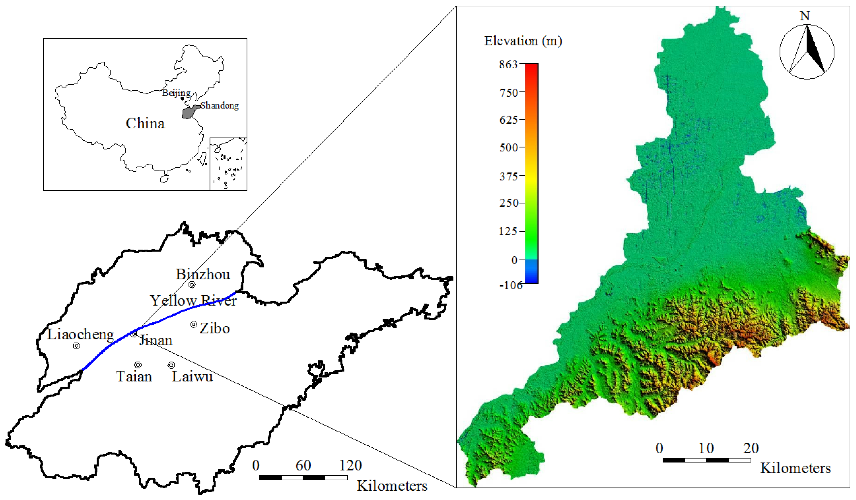
2. Description of Study Area

The Jinan karst aquifer system, a monoclinic structure which is in the karst area of northern China, covers more than 2614 km2 north of Tai Mountain in Shandong province (Figure 1). The climate of Jinan is classified as medium latitudes monsoonal with an average annual rainfall of 673 mm and evaporation of 1175.8 mm. The topography of the Jinan karst aquifer system gradually drops in elevation from south to north, displaying changes from hilly land to a piedmont inclined plain, and further to the Yellow River alluvial plain. Precipitation is the main recharge source of the karst aquifer system. The main aquifers in the groundwater system are Ordovician limestone and oolitic limestone. The karst groundwater generally flows from south to north, which is basically controlled by the dip direction of karst strata and topography. Groundwater flow is obstructed by impermeable Mesozoic igneous rocks (diorite and gabbro) or Carboniferous-Permian sandstone and shale in the north of the groundwater flow system. In the suitable areas of topography and structure, the confined karst groundwater flows out as ascending springs, with a typical monoclinic artesian structure. Under natural flow conditions, these forms form well-known Jinan spring groups, such as the Baotu Spring, the Black-Tiger Spring, the Pearl Spring, and the Five Dragon Lake. In addition, porous aquifer of the loose sediments is mainly distributed in the intermountain valley, alluvial plain in the Piedmont, and areas along the Yellow River.

3. Methodology

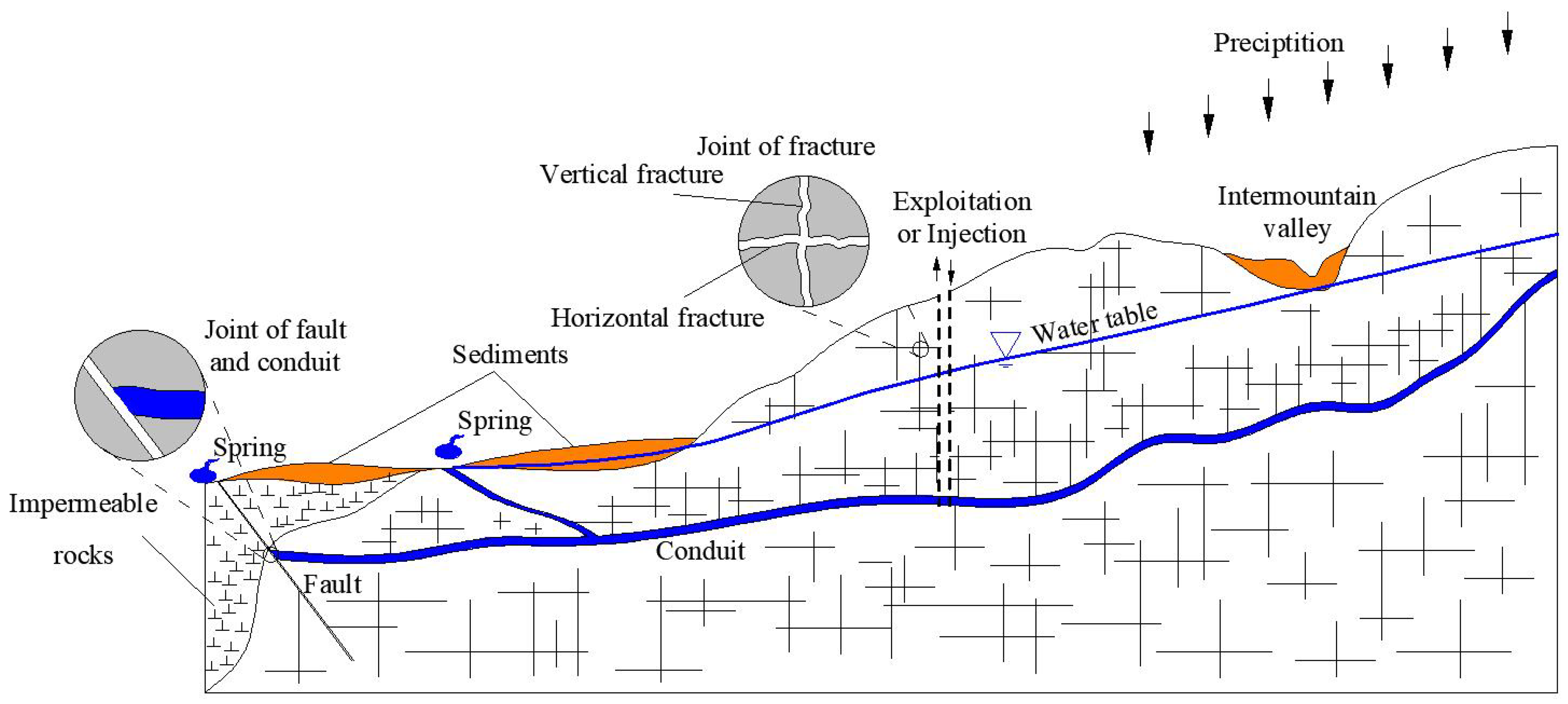
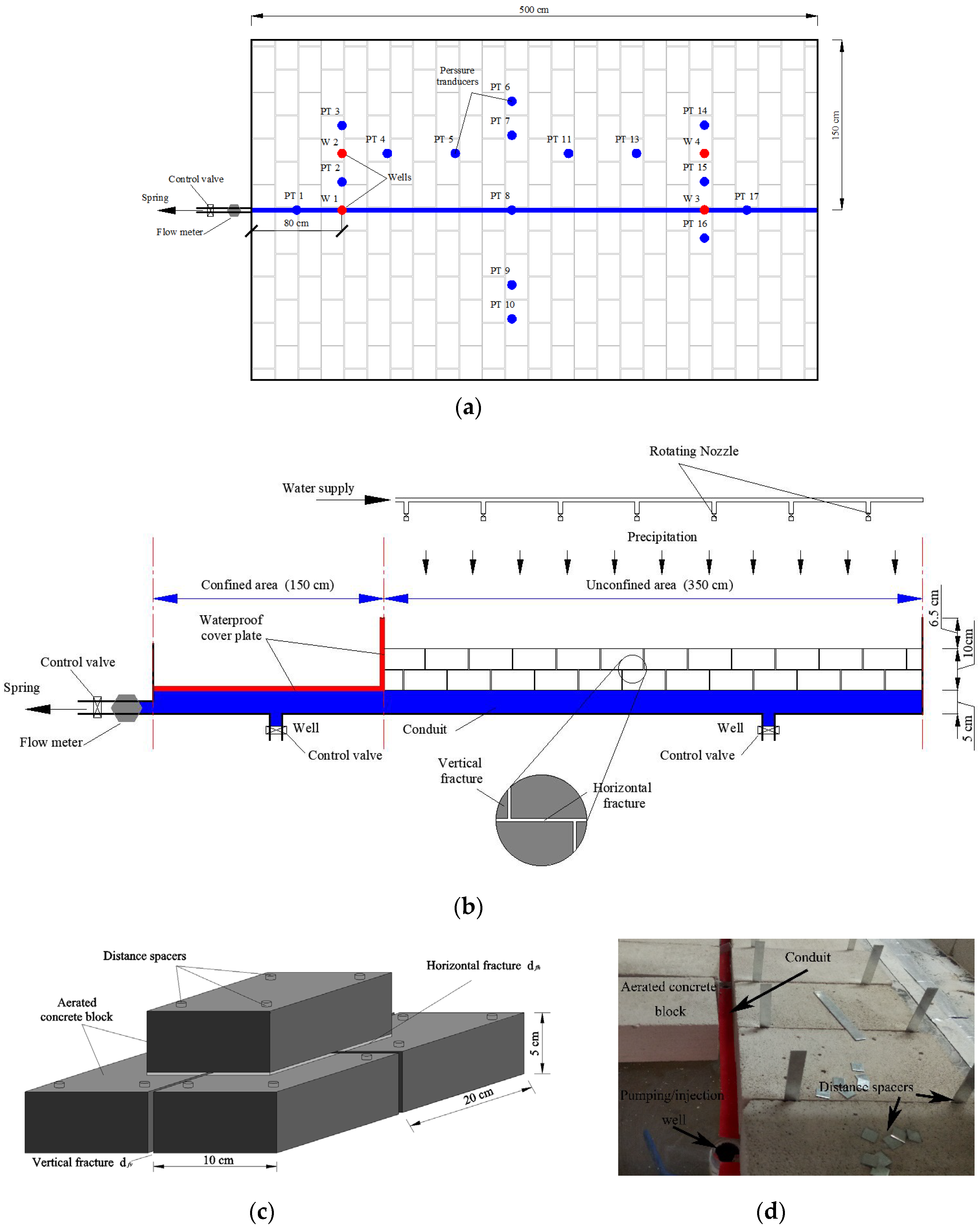
3.1. Conceptual Model and Laboratory Experiments

Figure 2 provides a two-dimensional sketch of the conceptual model proposed of the Jinan karst aquifer system. The karst aquifer system consists of conduits and fissures. The boundary of the conceptual karst system is divided into the spring, precipitation, and the ignored evaporation when groundwater flow process is monitored on a short-time scale. Groundwater flow in the conduit is confined or unconfined, which connects the spring. Surrounding the conduit is a fissured medium, such as fractured limestone. In addition, a quaternary porous medium covers the karstic medium in some areas. The karstic medium and porous medium are regarded as the matrix holding water. As a result of the continued dissolution and erosion during the geologic history and because of the arid Quaternary and present-day dry climate, karst development in this area becomes well-developed with increased depth, shown in Figure 2.
Laboratory experiments were carried out in a physical model based on the conceptual model shown in Figure 3. The physical model is composed of karst medium, precipitation system, hydraulic head collection system, and spring flow monitoring system. The physical model was constructed of acrylic glass with the dimension 5 m (length) × 3 m (width) × 0.5 m (height) (Figure 3a,b). The physical karst aquifer model was divided into confined and unconfined areas. The fissures and conduit areas were built using aerated concrete block (Figure 3c,d) separated by distance spacers with different thickness, that is, fissure distance spacers (including horizontal fissures and vertical fissures) in the experiments were df = 0.7 mm; size of conduit section was 5 cm (height) × 2 cm (width). The size of fissure distance spacers was set according to the results of Zhang et al. [45], who showed that a closed flow structure with less than 1.4635 mm aperture could be defined as a fracture while a closed flow structure with more than 1.8375 mm aperture could be defined as a conduit. The height of the spring opening was set to be 0.05 m above the bottom of the tank. To ensure that the downstream area is a confined aquifer, the initial head in the tank was also set to be 0.05 m. Four computer-controlled pumps, with a maximum pumping rate of 2 L/min, were installed in four wells (W 1–4) (Figure 3a). Discharge and recharge rates were observed continuously. A total of seventeen (Figure 3a) high-sensitivity (AE-T, by Nanjing AE Sensor Technology Co., Ltd., Nanjing, China) deflated pressure transducers (PTs) were buried into the bottom of the physical model to measure hydraulic heads. These PTs were connected to a time-synchronized data-logger that collected measurements once per second. A total of twenty-one rotating nozzles with a spray angle of 360° were installed on the steel frame above the recharge area. Rainfall intensity was controlled by a variable frequency pump with a flux of 0–15 m3/h. A PVC tube controlled by a valve was connected with the outlet of the conduit to represent spring. The discharge elevation of spring was variable, and the flow flux was monitored by an ultrasonic flowmeter (MIK-2000H, XIANGRUIDE Co., Ltd., Nanjing, China) with a measuring accuracy of ±1%.

3.2. Scenarios Definition

Three different artificial regulated conditions were considered as hydrological scenarios (Table 1, Scenarios A–C). Scenario A represents a hydrological condition with no artificial recharge and no groundwater exploitation. Scenario B and Scenario C represent the hydrological condition with constant pumping rate (pumping well) and artificial recharge rate (injection well), respectively, applied at different locations. Four different pumping/injection locations (Figure 3a) and three different pumping rates (0.5 m3/day, 1.0 m3/day, and 1.5 m3/day) and injection rates (1.5 m3/day, 2 m3/day, and 3 m3/day) were applied in Scenario B and Scenario C to examine the effect of artificial regulation on the spring hydrographs. A constant precipitation rate was applied to the surface of the unconfined area at 2 m/day for a period of 1000 s for each experiment.

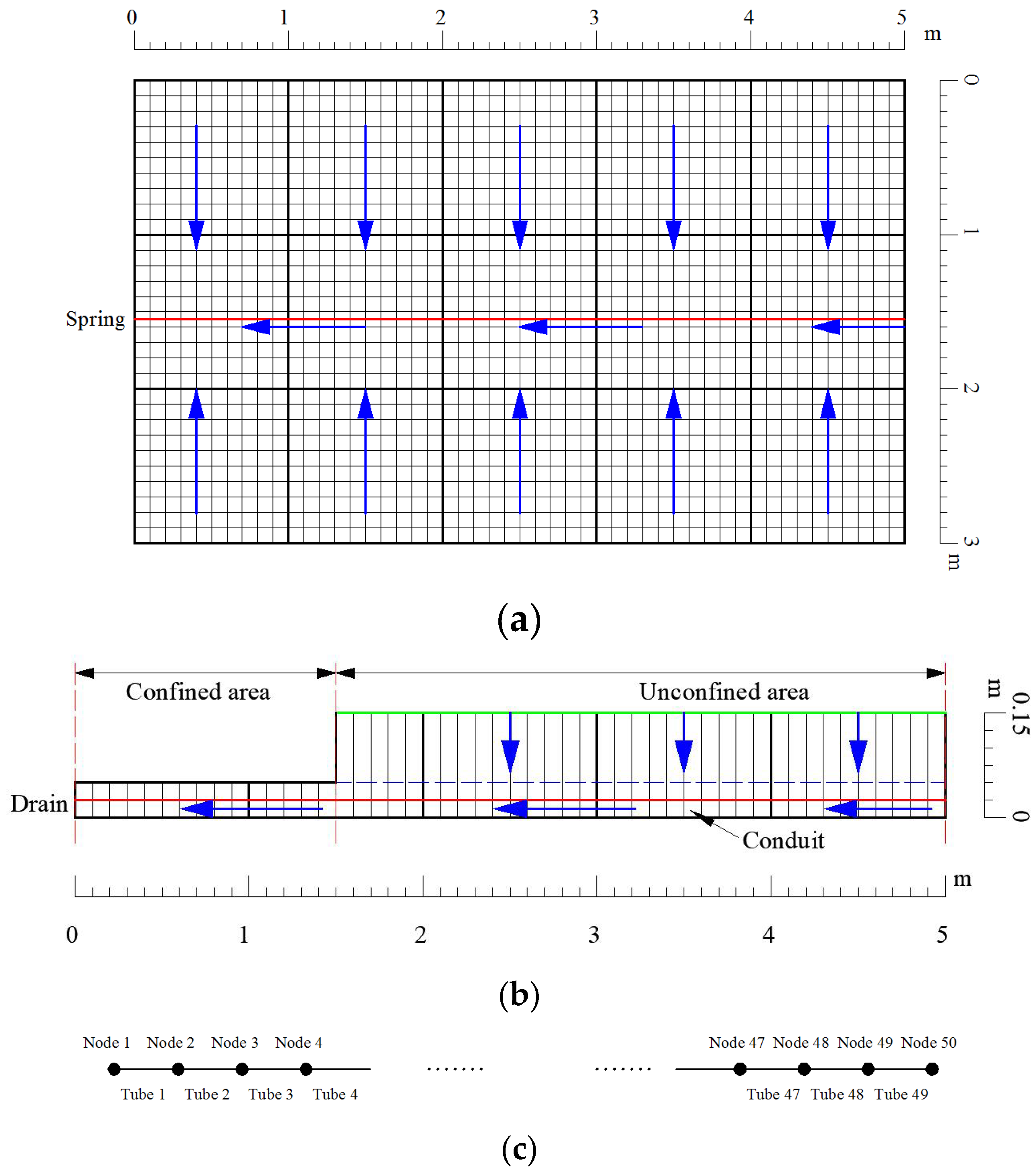
3.3. Numerical Model

A corresponding numerical model with a single conduit surrounded by low permeability 2-D fissure zone was considered. The fissure zone of the model was 5 m long and 3 m wide, and the width of both columns Δx and rows Δy was set to 10 cm for each cell (Figure 4a). The fissure zone was defined as an unconfined layer with a thickness of approximately 0.15 m and a confined layer with a thickness of approximately 0.05 m (Figure 4b). The elevation of the aquifer bottom was set to 0 m. There are no-flow boundaries around the fissures zone and a Neumann-type boundary for the unconfined aquifer surface. The 4.9 m long conduit was in the middle of the fissures zone (15th row) and discretized in 0.1 m long elements. There were 50 conduit nodes and 49 tubes with their numbers increasing successively from left to right (Figure 4c). Conduit Node 1 was set to a constant head boundary with the fixed head 0.05 m to represent a spring (Figure 4). The initial head of the model was also set to be 0.05 m. According to the conceptual model and laboratory physical model, precipitation only recharges the fissures zone in the model. None of the conduit nodes receive recharge. The corresponding numerical models described herein represent typical karst aquifers without allogenic or point recharge on the conduit. The fissures receive the precipitation which is discharged by the conduit to the spring.
Modflow-CFPM1 (CFP model 1) was used for the numerical simulations. The low permeability fissure zone was conceptualized as an equivalent porous media [17], and groundwater flow in the fissure zone was described by a partial differential equation [46].
x ( K x x h m x ) + y ( K y y h m y ) + z ( K z z h m z ) ± W = S s ( h m t )
where Kxx, Kyy, Kzz are the hydraulic conductivities (LT−1) along the x, y, and z-axes, respectively, hm is the groundwater head of the fissures zone (L), W is the external volumetric flux per unit volume and represents sources or sinks of water, including the recharge and well pumping (T−1), Ss is the specific storage (L−1), and t is the time (T).
Flow in cylindrical conduits could be laminar or turbulent. The Hagen-Poiseuille equation was used to describe the laminar flow in the conduit.
Q = A ρ g d 2 Δ h c 32 μ Δ l τ
where A is the flow cross-sectional area of the conduit (L2), ρ is the density of water (ML−3), d is the conduit diameter (L), g is the gravitational acceleration constant (LT−2). v is the kinematic viscosity of groundwater (L2T−1), hc is the water pressure head in the conduit (L). τ is the tortuosity (unitless) of the pipe.
Turbulent flow in a conduit was represented by the Darcy-Weisbach equation with the Colebrook-White equation as:
Q = | Δ h c | g d 5 π 2 2 Δ l τ l o g ( 2.51 v 2 | Δ h c | g d 3 Δ l τ + k c 3.71 d ) Δ h c | Δ h c |
kc is the roughness factor which represents the mean roughness height of the micro-morphology of conduit wall (L).
The conduit network was coupled to the fissure zone with an exchange flow boundary. The linear equation used by the CFP to compute the exchange of groundwater between the fissure zone and conduits was given by:
Q e x = α e x ( h c h m )
where Qex is the volumetric exchange flow rate, α e x is the exchange coefficient between conduit and fissures zone cell.

4. Results

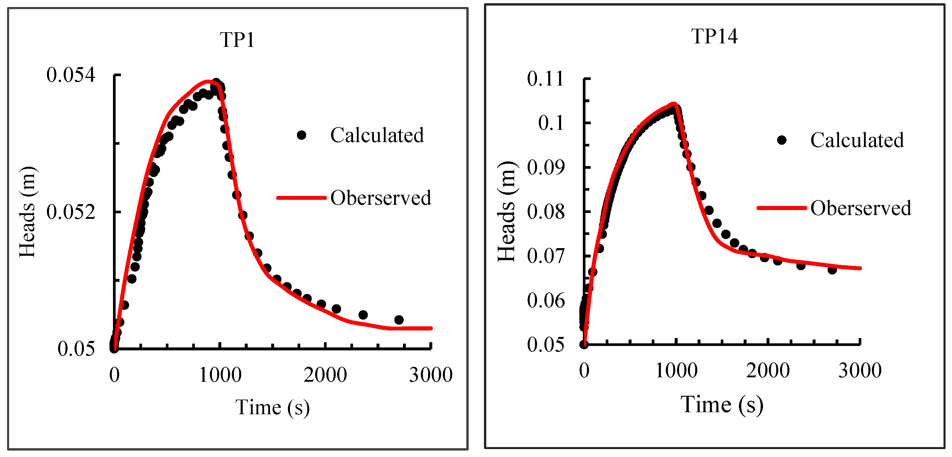
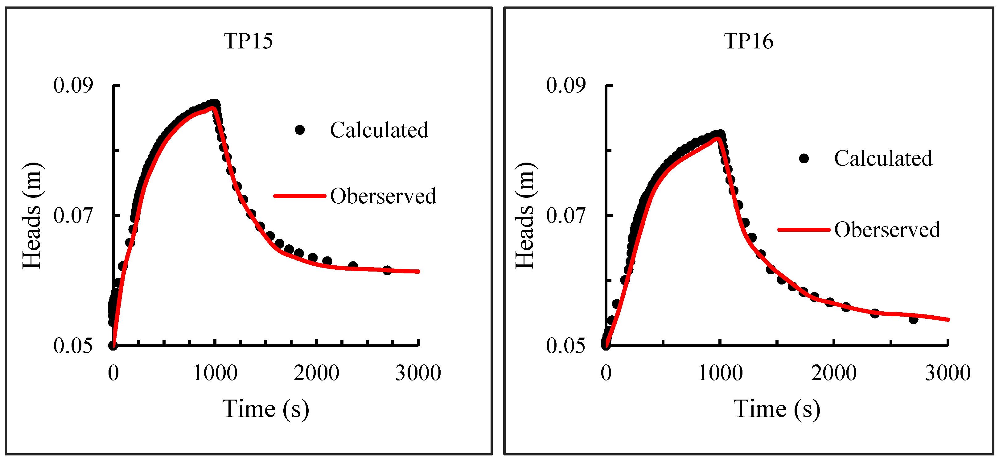
4.1. Laboratory-Scale Numerical Model Calibration

A laboratory-scale numerical model was calibrated to improve the fit between the observed and simulated groundwater head time series at seventeen observation points (Figure 3a). Scenario B, with a constant injection rate of 1.5 m3/day at W4, was used for model calibration. The first 1000 s were considered as the precipitation period, and the next 2000 s were the recession period of spring hydrographs after precipitation events.
Measured hydraulic head data images from scenario B were used to calibrate the model. In particular, the hydraulic conductivity and specific yield in fissures zone value were adjusted slightly using observed heads (Table 2). As an example, Figure 5 shows the fitness between the measured head and calculated head by the trial-and-error calibration method, and the good fitness indicates that the numerical model was reliable for its application.

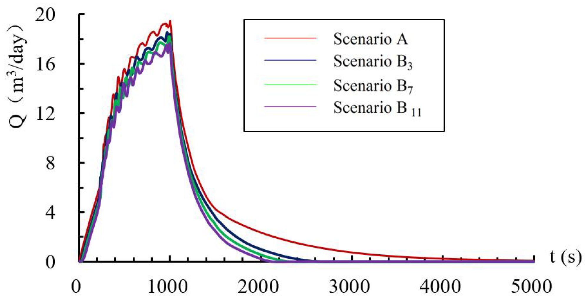
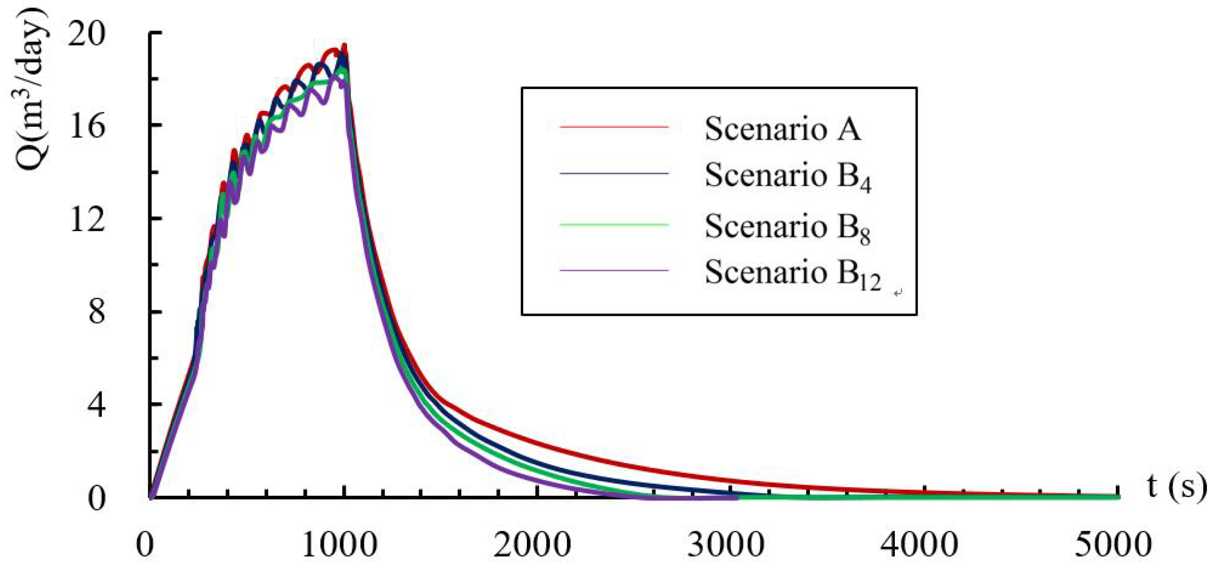
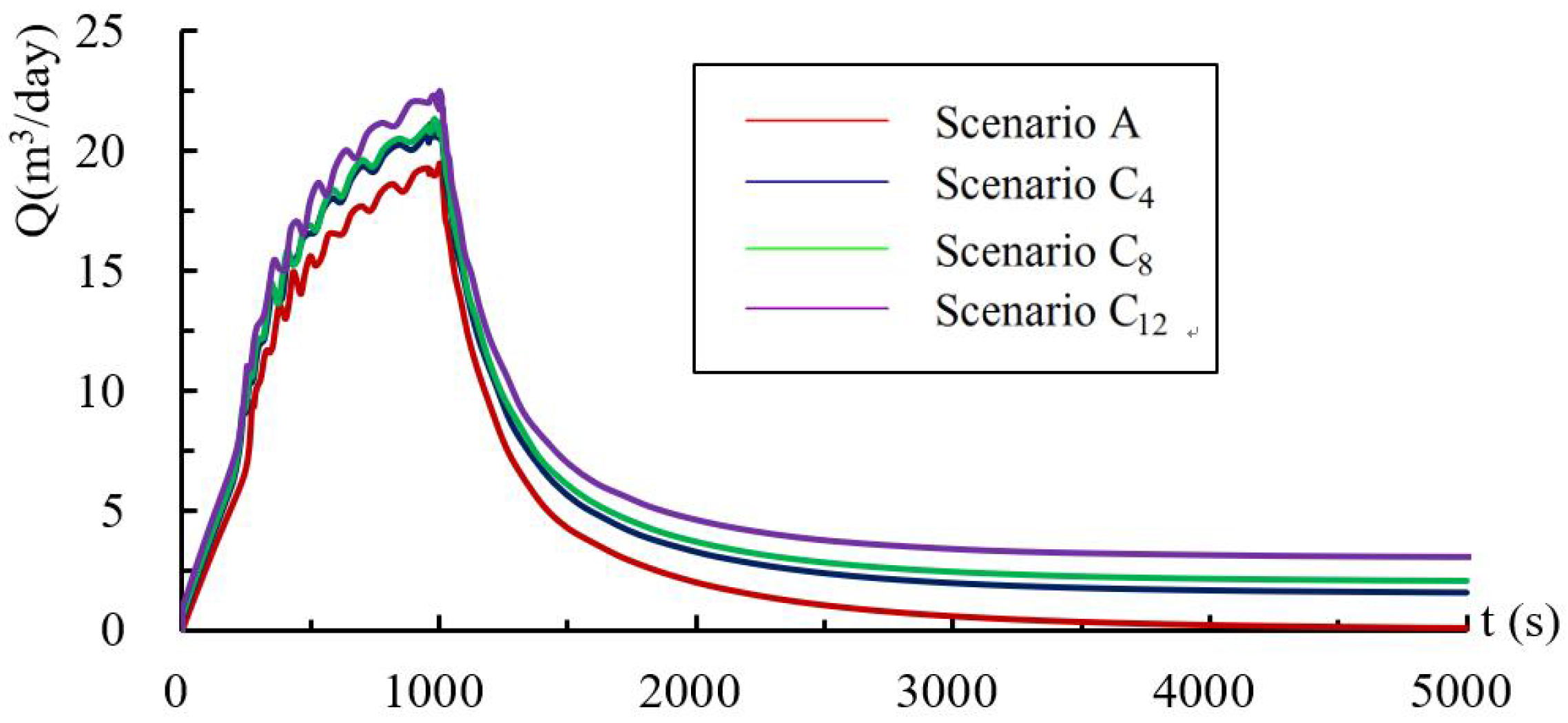
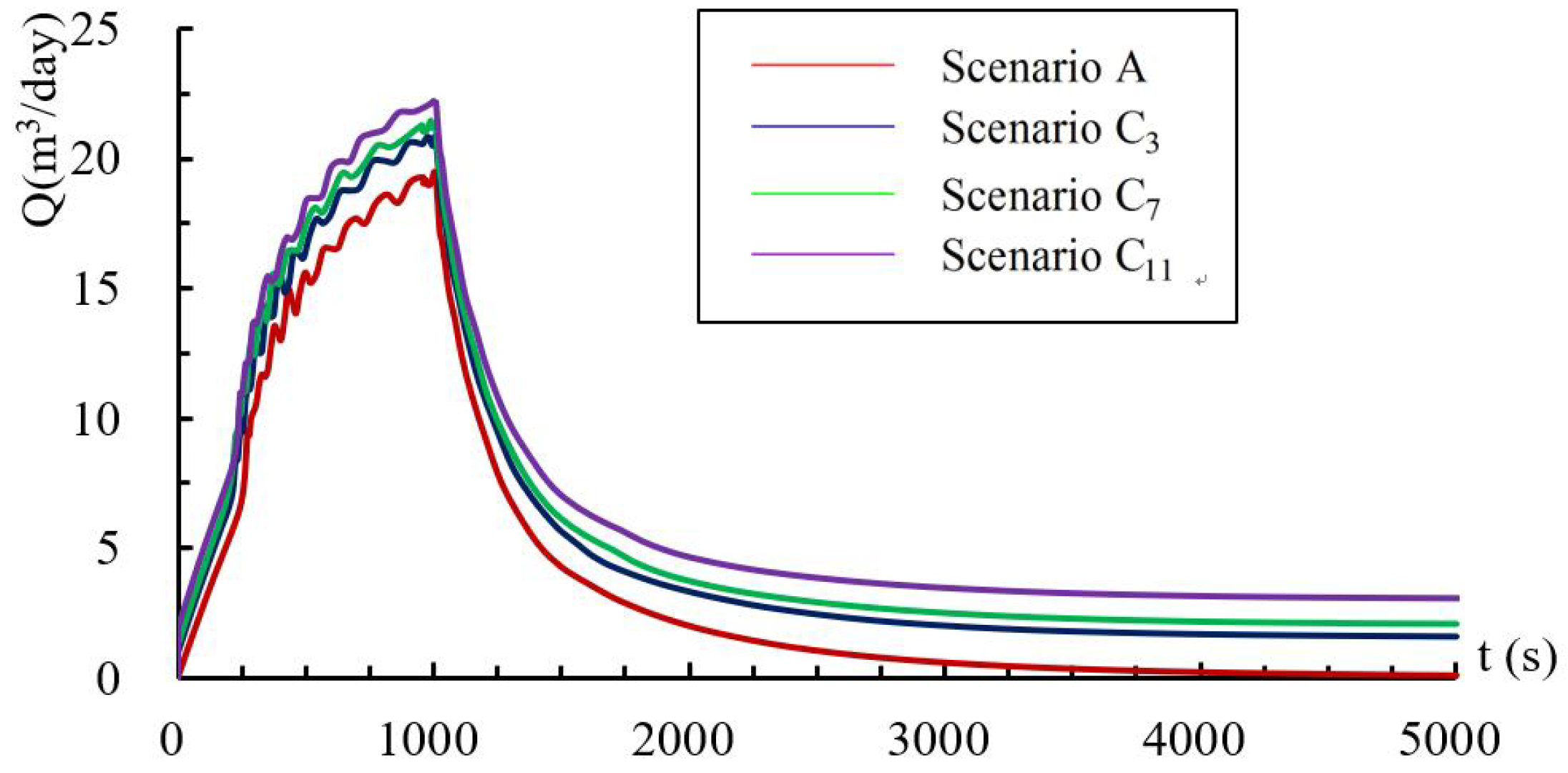
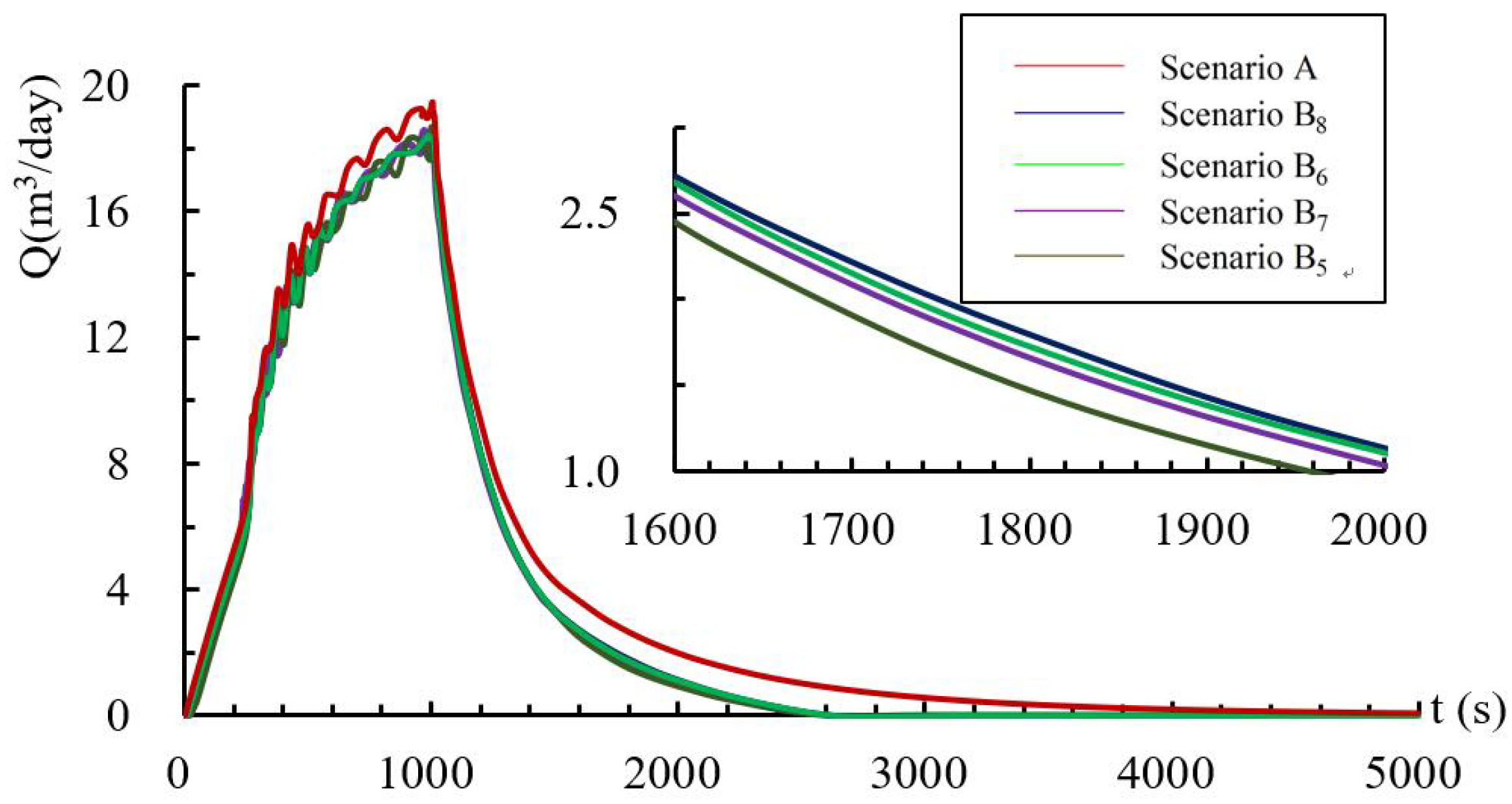
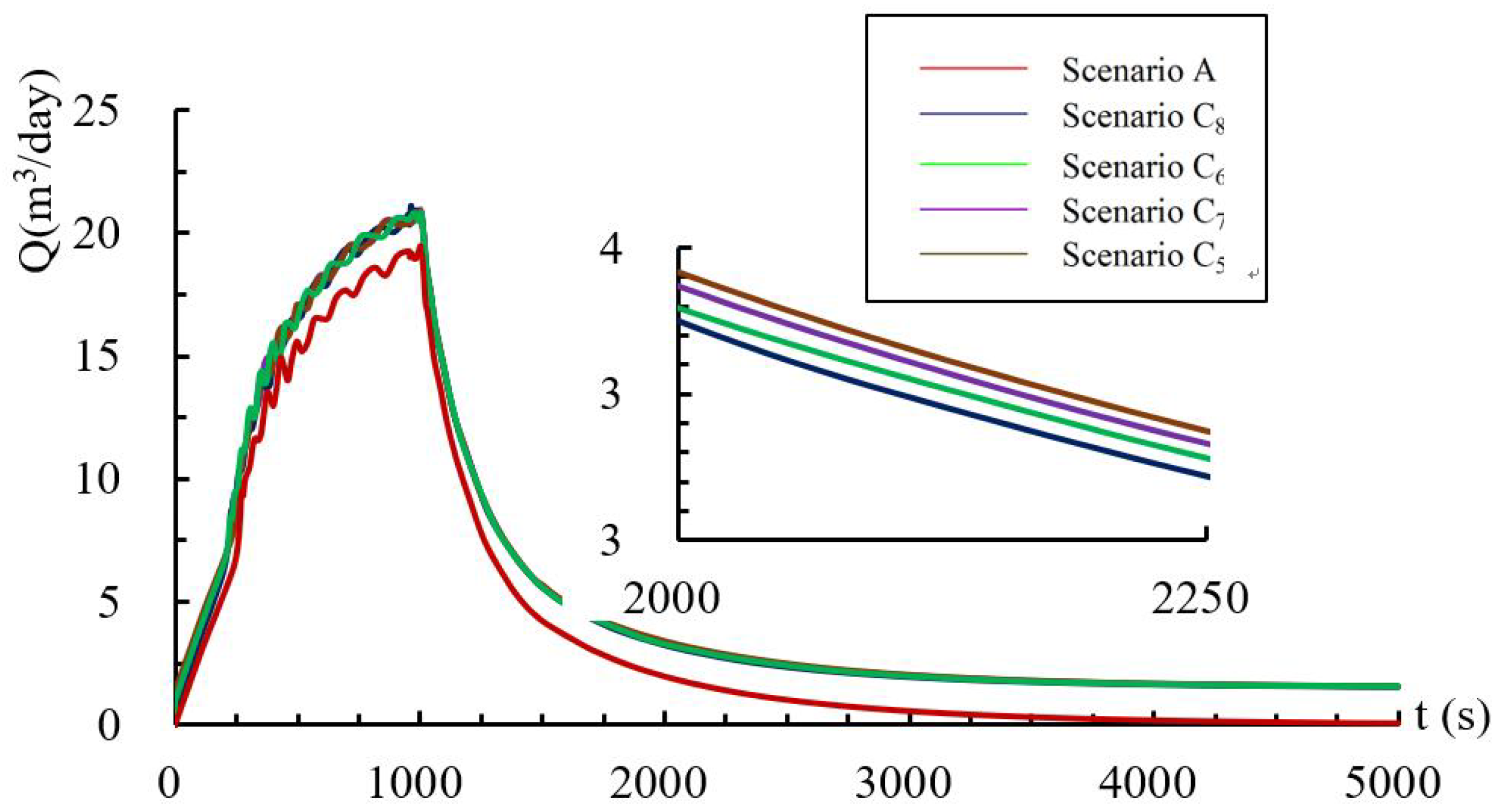
4.2. Effects on Spring Hydrographs

Figure 6, Figure 7, Figure 8, Figure 9, Figure 10 and Figure 11 show the spring hydrographs driven by different artificial regulation modes at wells W1, W3 at the conduit zone and wells W2, W4 at the fissure zone (Figure 3a). The spring hydrograph peaks decreased gradually with the increase of pumping rate but increased with increased injection rates at both the fissure zone and conduit zone (Figure 6, Figure 7, Figure 8 and Figure 9). The spring discharge and recession time decreased with increased pumping rate in both fissures zone and conduit zone and increased with the increased injection rate (Figure 6, Figure 7, Figure 8 and Figure 9). Figure 10 and Figure 11 show the results of spring hydrographs influenced by pumping and injection at different locations (Figure 3a) with constant pumping or injection rate, indicating minimal changes in the spring hydrographs peak with the transferring of wells positions. The effect of the position of a well, including pumping wells and injection wells, on the spring discharge occurred mainly during the recession period of spring hydrographs. As shown in Figure 10, spring discharge and recession times decrease with the transferring of pumping well from fissures zone to conduit zone. The closer the pumping locations to the spring, the greater the decrease in spring discharge and recession time. As shown in Figure 11, injection in conduit zone increases the spring discharge and recession time compared to injection in the fissure zone. In addition, the closer the injection locations to the spring, the greater the increase in spring discharge and recession time.

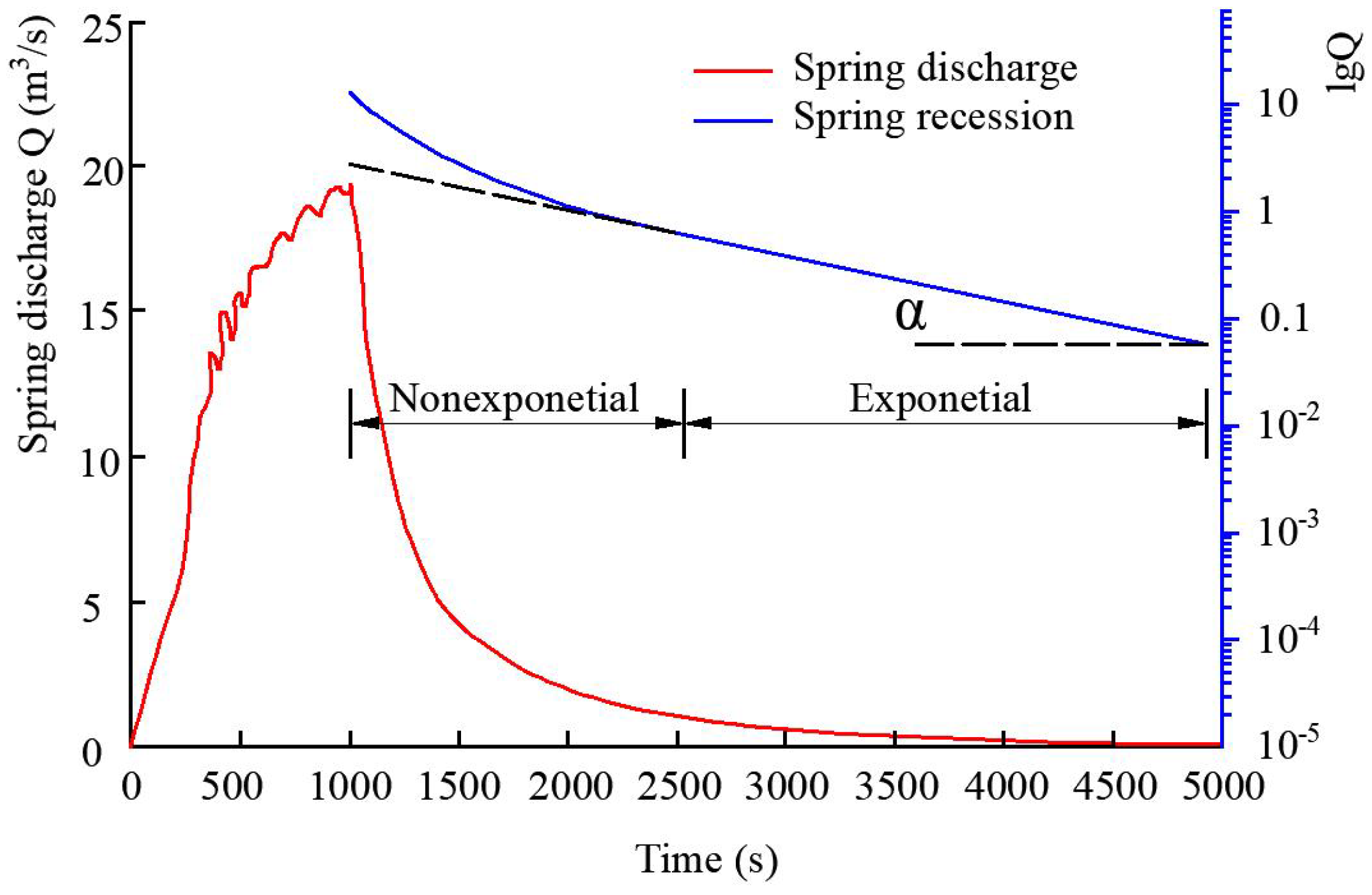
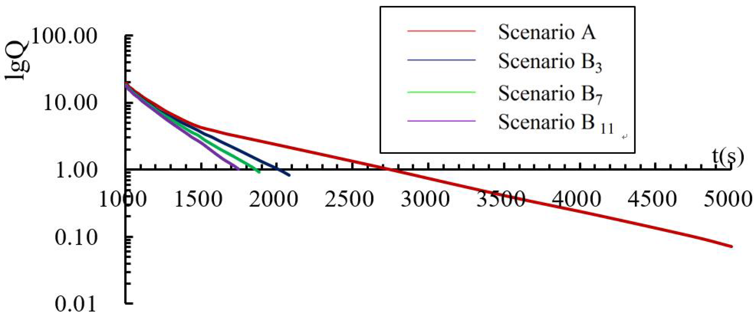
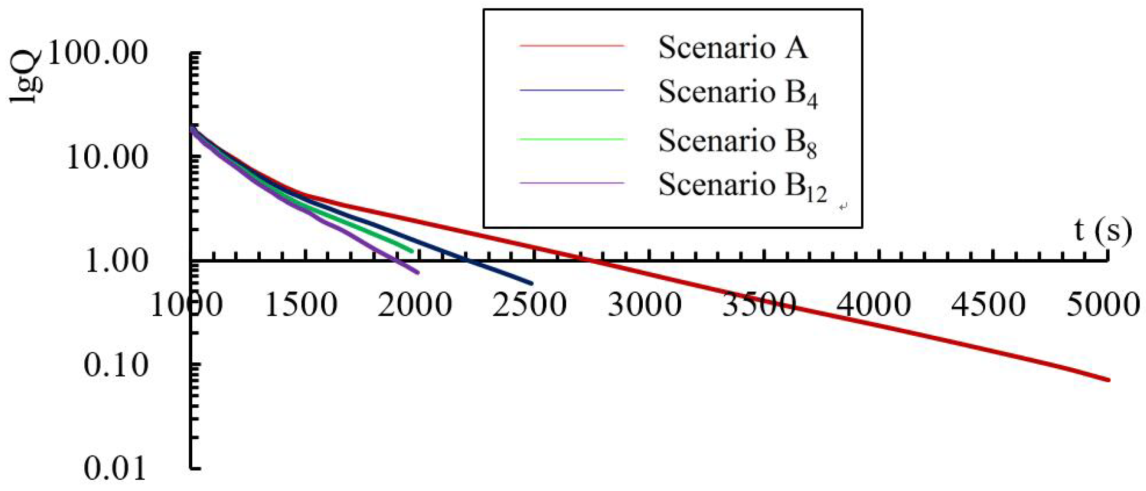
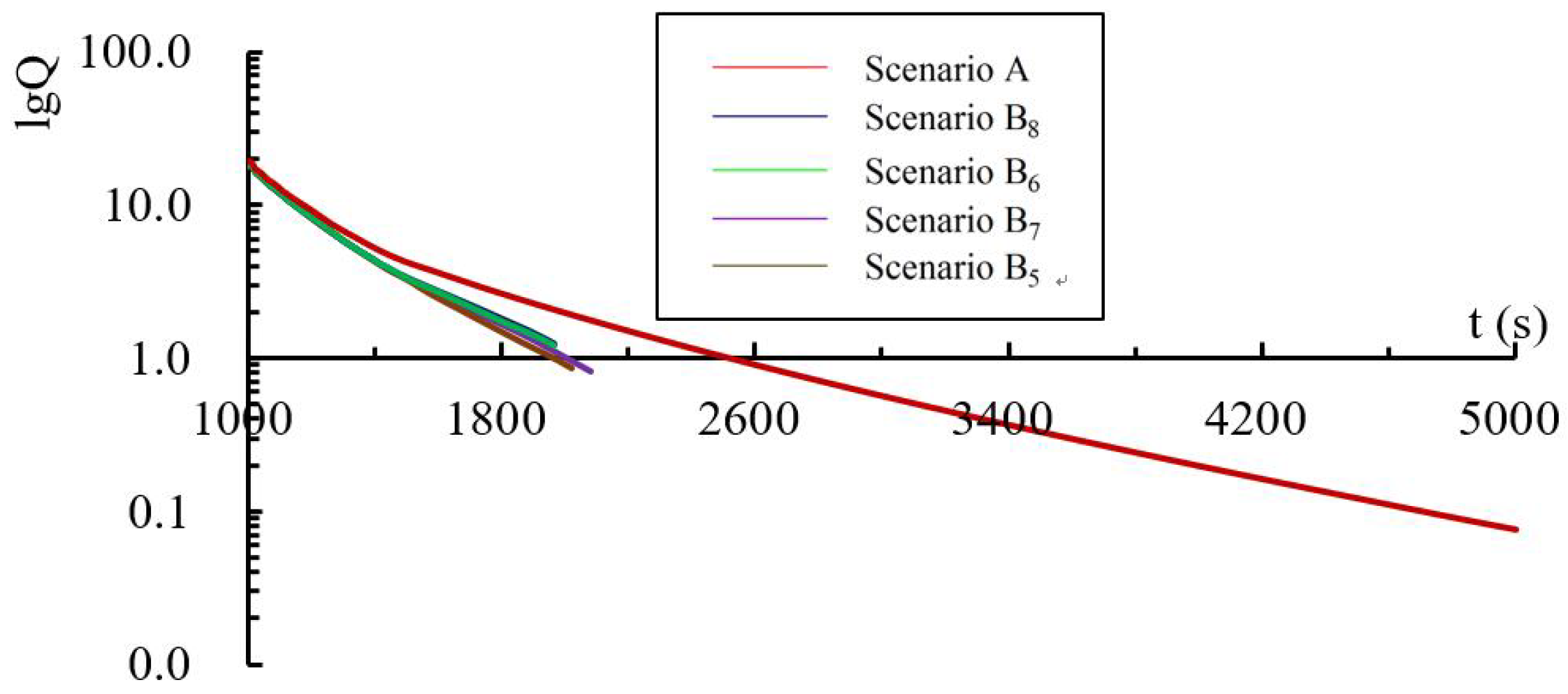
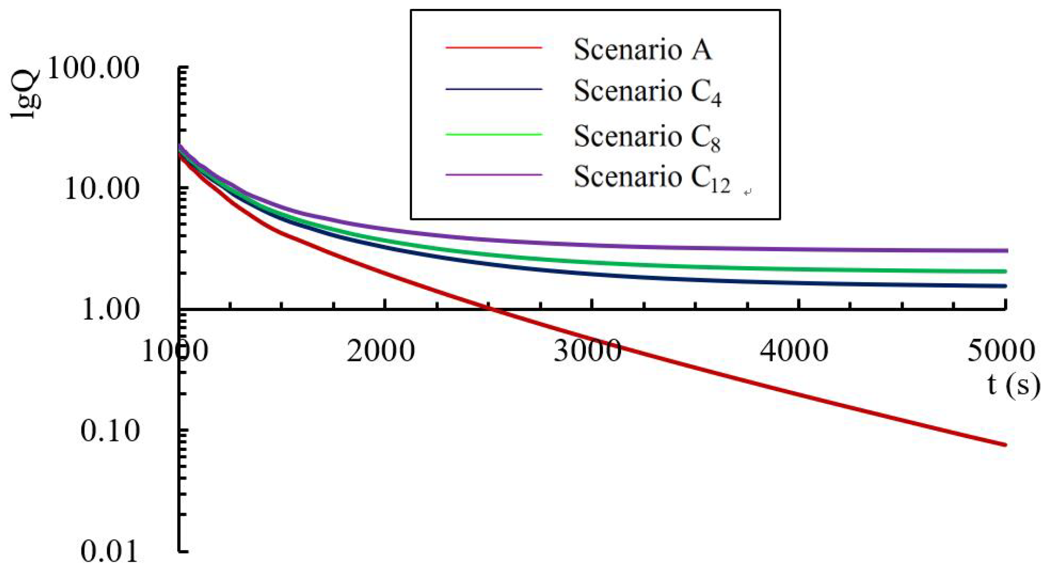
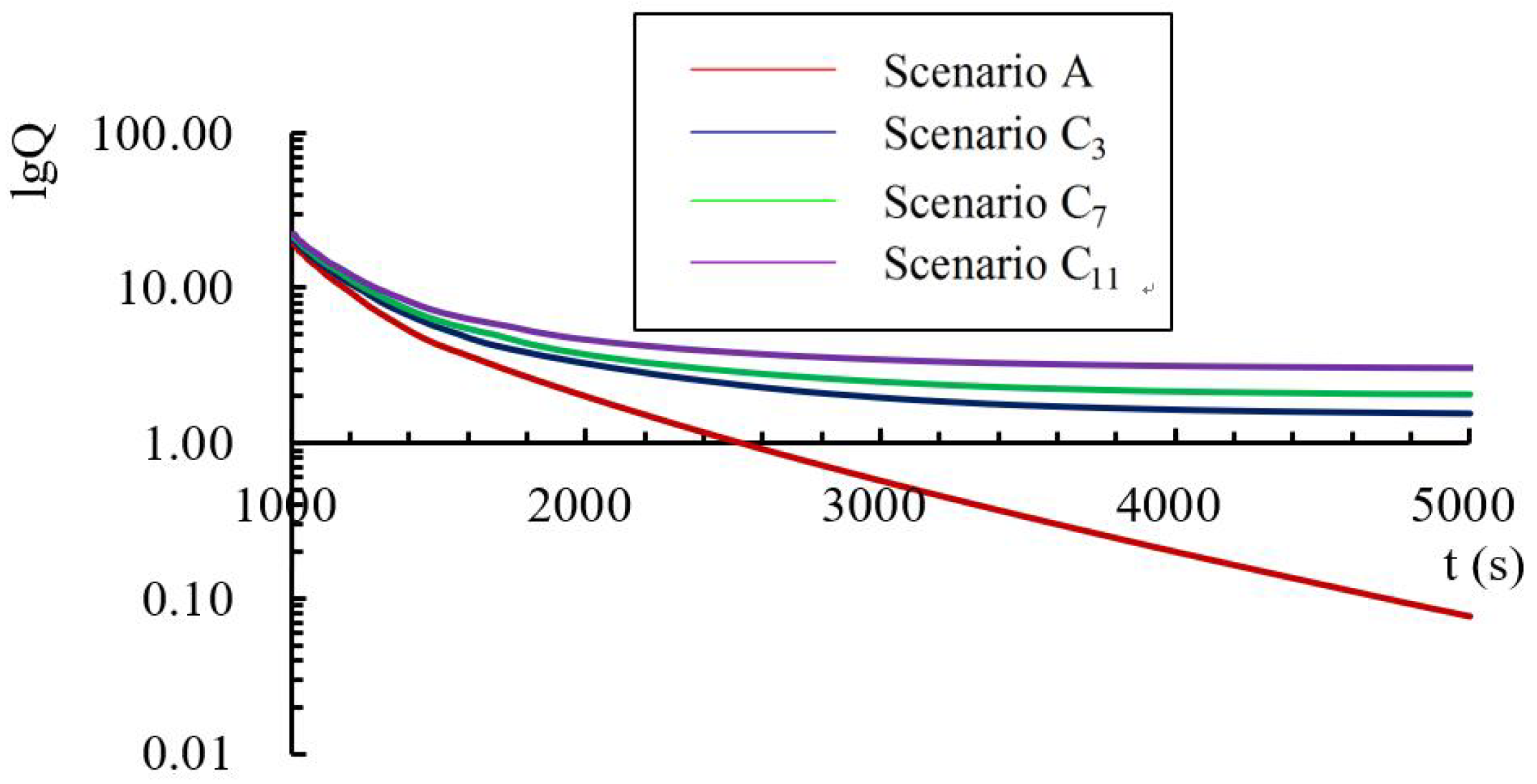
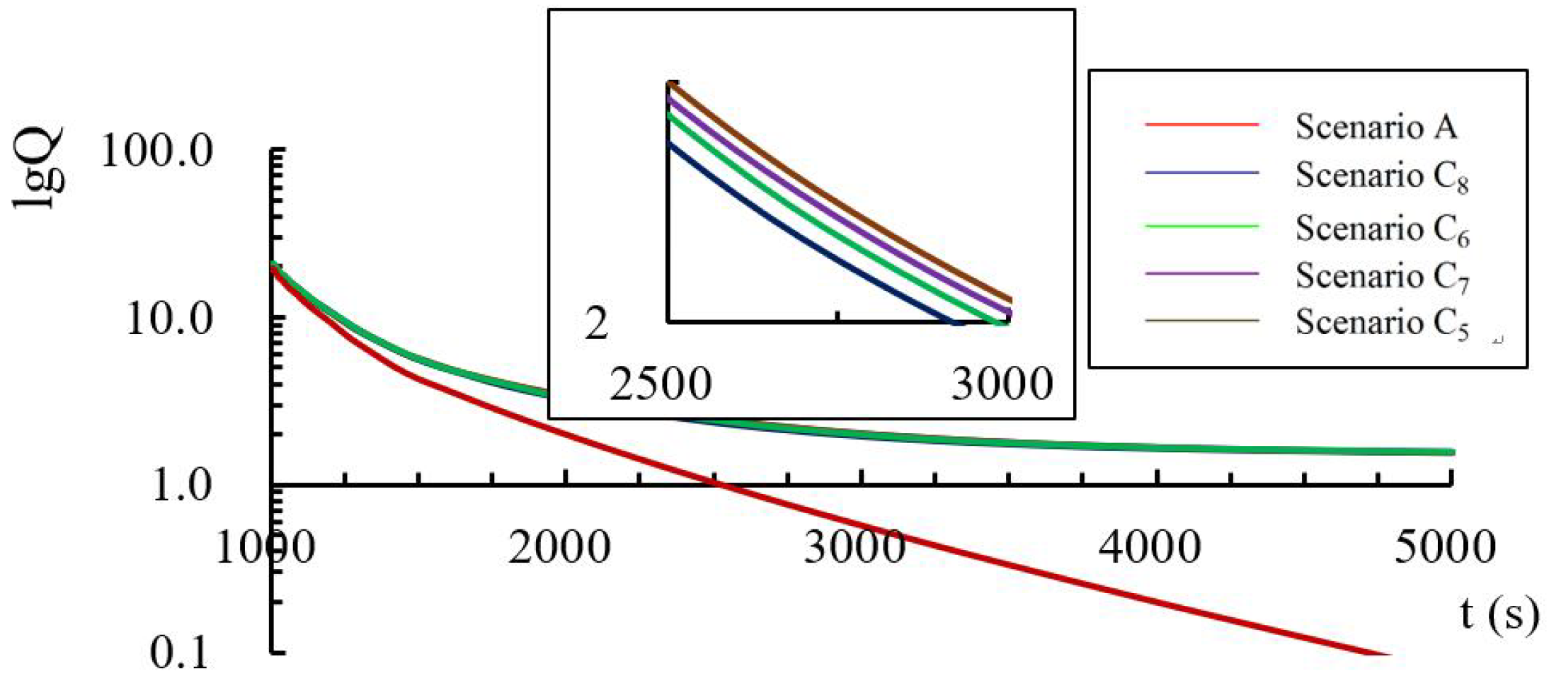
4.3. Effects on Recession Curves

Recession curves are typically plotted in logQ-t space to illustrate the division of sub-recession curves and calculation of recession coefficient (Figure 12). Sub-recession curves plot as straight lines in logQ-t space when the spring discharge decreases exponentially with time. The slope of the straight line is the recession coefficient. Non-exponential sub-recession curves indicate as a nonlinear variation on the logQ-t plot, and the slope at a specific position provides the recession coefficient at this point. Obviously, the recession curve contained the early non-exponential sub-recession curve and late exponential sub-recession curve in a natural state in this study.
Figure 13, Figure 14, Figure 15, Figure 16 and Figure 17 show that spring discharge recession could be strongly influenced by different artificial regulation modes. However, the influences of different artificial regulating position on the recession behavior were not sufficiently distinctive in the laboratory experiment scale results (Figure 15 and Figure 18). Figure 13 and Figure 14 show the spring discharge recession at different pumping rates in fissure and conduit zones in upstream locations, respectively. Pumping at different models of karst media altered the recession coefficient, especially in the late sub-recession curves. Under the influence of pumping, the recession curve contained the early non-exponential sub-recession curve and late exponential sub-recession curve. However, increased pumping rates made the recession coefficient of late sub-recession curves approach the early sub-recession curves. Effects of different pumping locations on the recession curves are shown in Figure 15. Pumping in the conduit zone showed more obvious effects on the decrease of recession coefficient in the late sub-recession curves. In addition, the closer to the spring, the stronger the influence of pumping on the decrease of the recession coefficient of late sub-recession curves.
Figure 16 and Figure 17 show the spring discharge recessions influenced by different injection rates in fissure and conduit zones in upstream locations, respectively. Figure 16 and Figure 17 also indicate that the recession coefficient decreases with the increase of injection rates, especially in the late sub-recession period. Influenced by injection, the late sub-recession of spring discharge did not obey an exponential recessing law. Figure 18 shows the results of spring discharge recessions driven by changing injection positions at constant injection rates. Injection in the conduit zone showed more obvious effects on the increase of the recession coefficient in the late sub-recession curves. Besides, the closer to the spring, the stronger the influence of injection on the increase of the recession coefficient of late sub-recession curves.

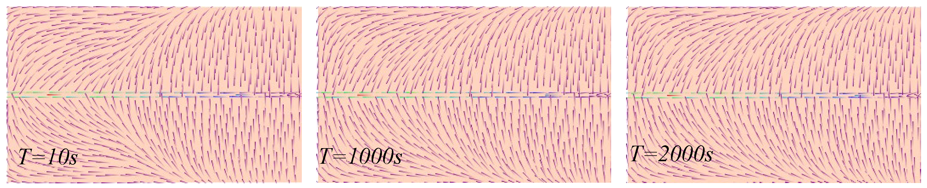
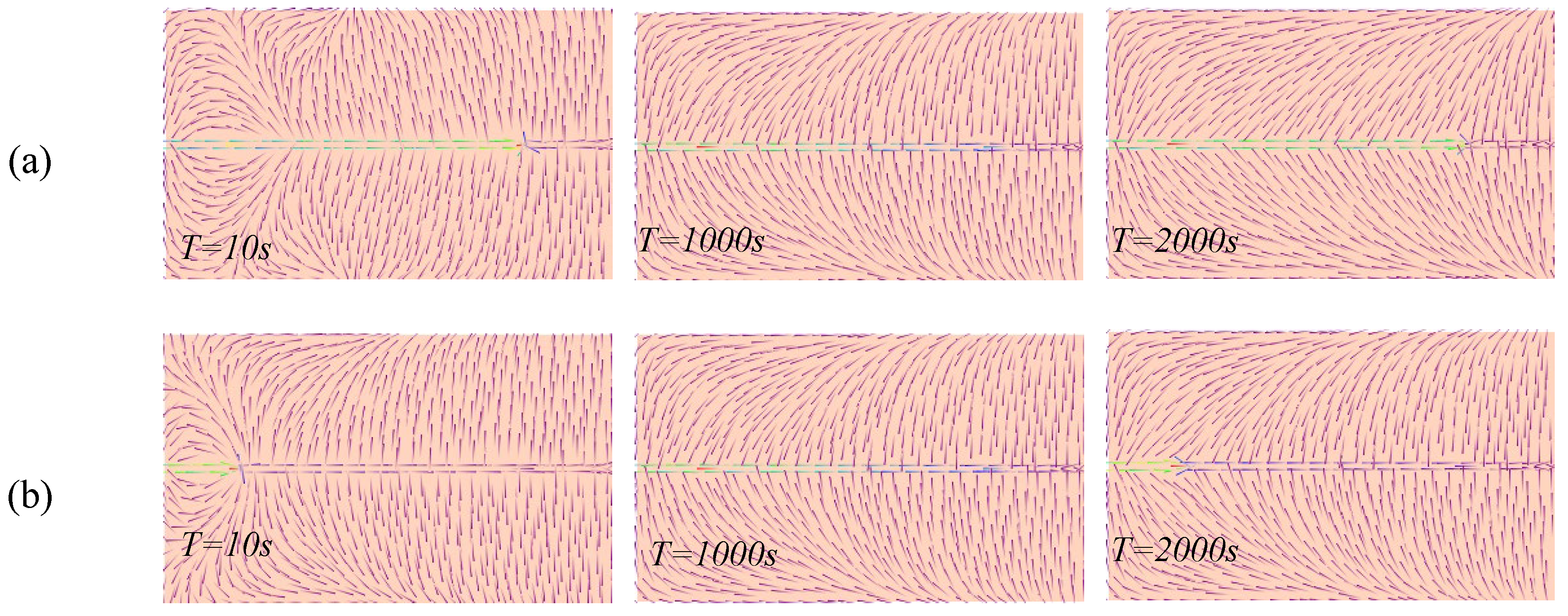
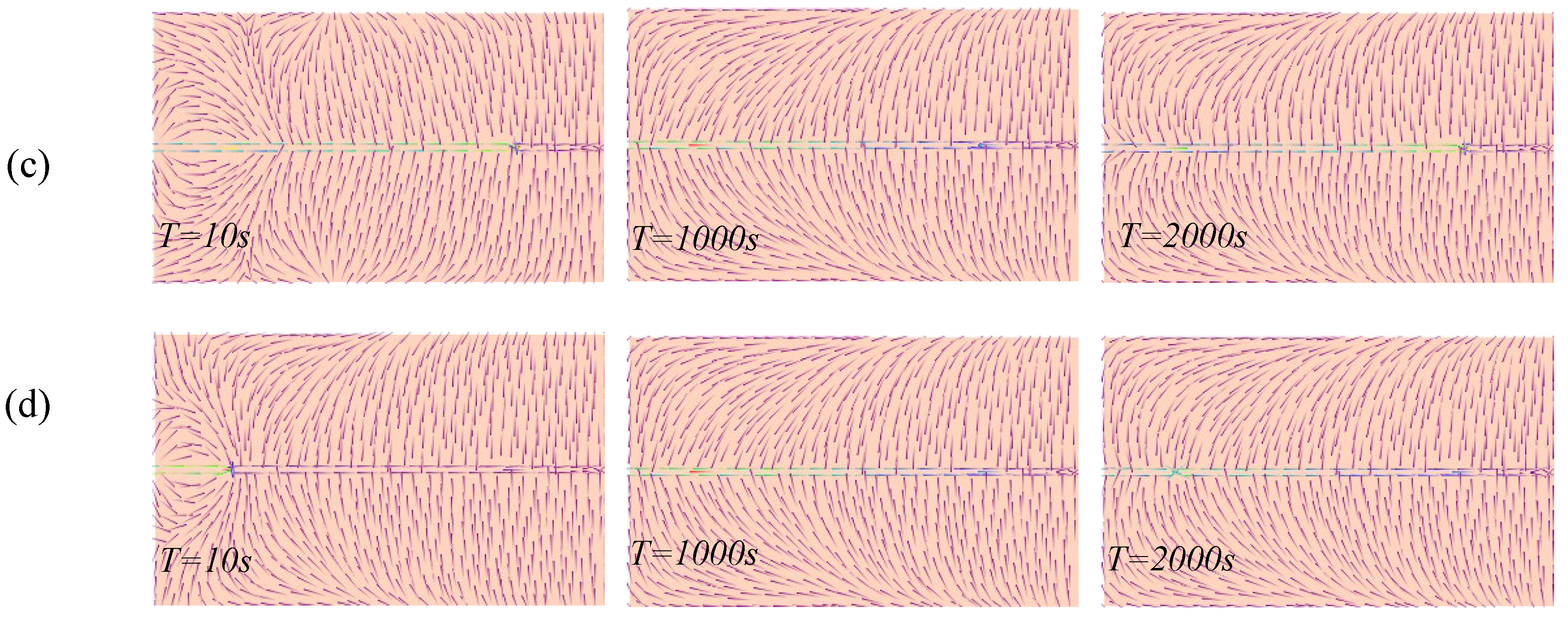
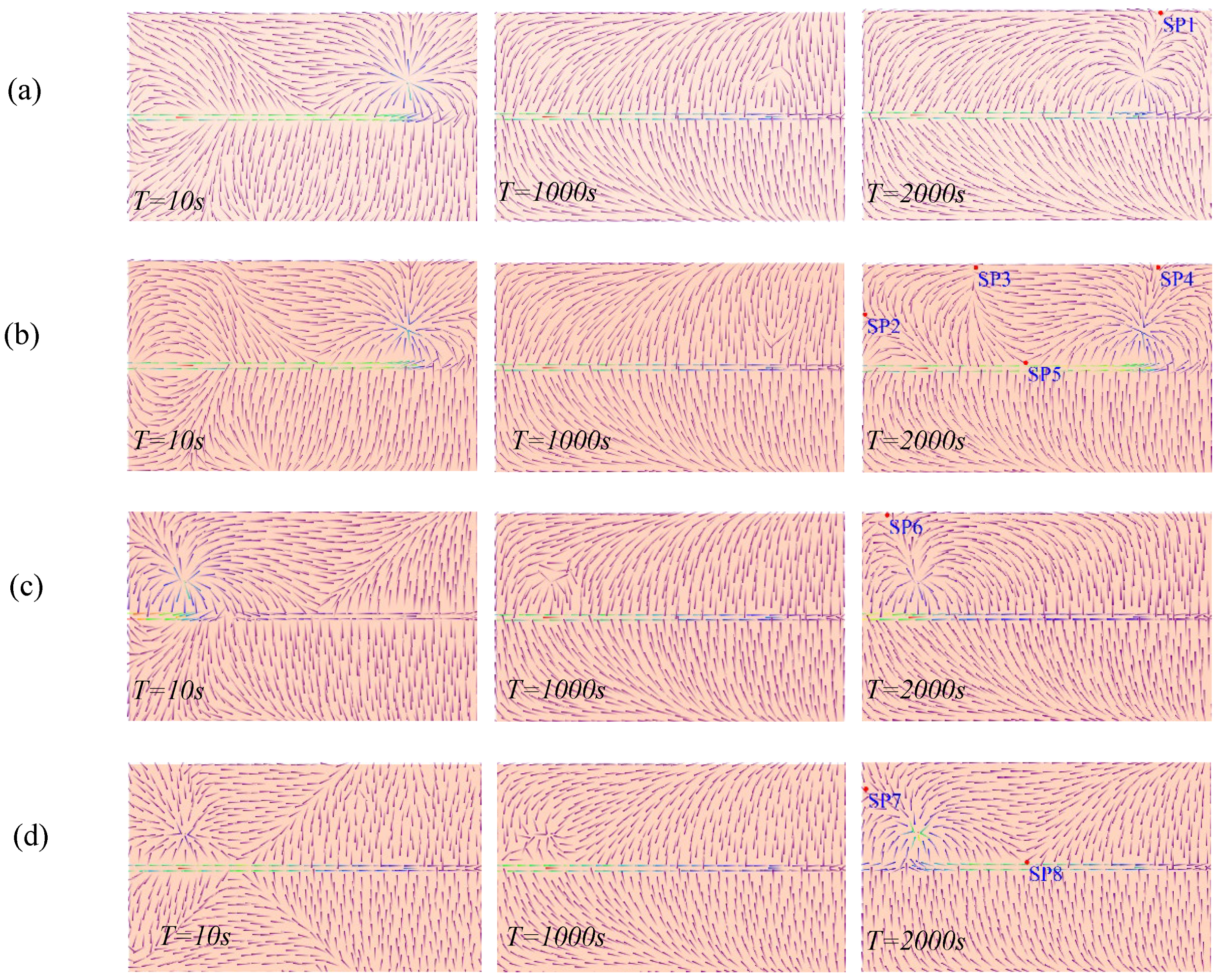
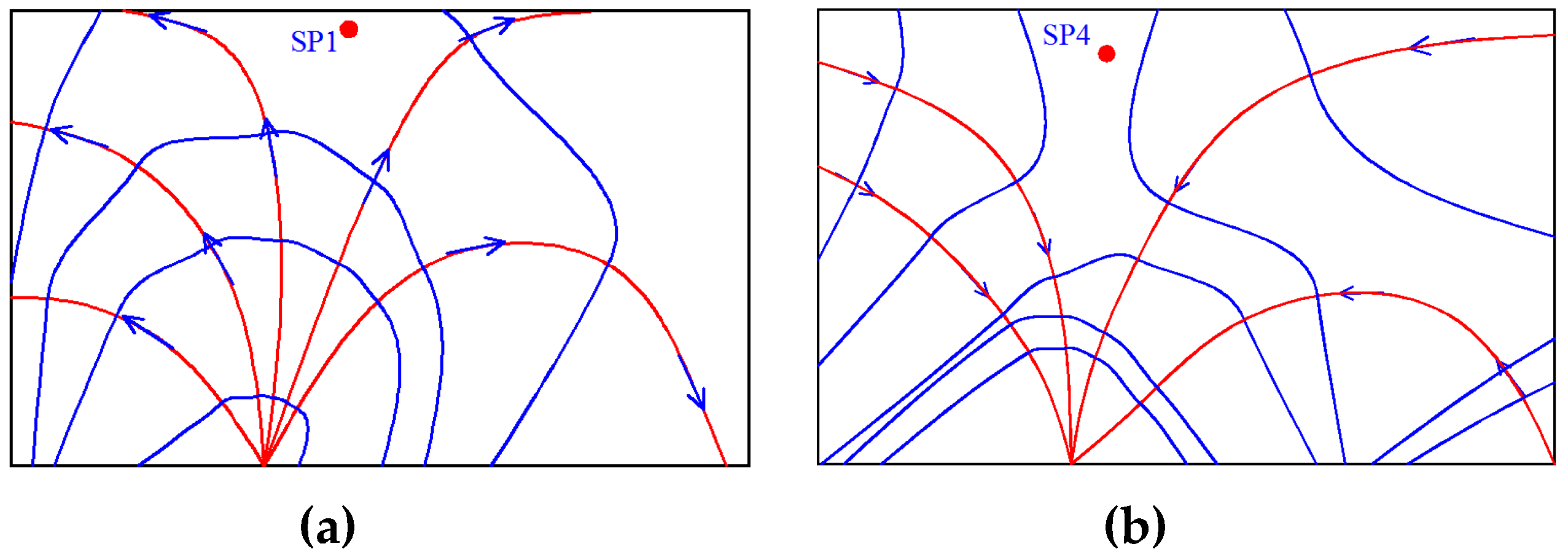
4.4. Effects on Groundwater Flow Dynamics

The variation of groundwater flow dynamics for different scenarios is shown in Figure 19, Figure 20 and Figure 21, which indicate that the exchange of groundwater between conduits and fissures zone is different from each other for different artificial regulation modes. With the effect of artificial regulation, a complicated conversion relationship between the conduit and fissures zone emerged during the test process. Simulation results showed that for scenario A (Figure 19), without artificial regulation, the direction of groundwater flow was mostly from the conduit zone to the fissures zone. Flow directions were mostly perpendicular to the conduit in the upstream areas. With the extension of the test duration, areas which represent flow direction perpendicular to the conduit gradually expanded.
Figure 20 shows the flow fields regulated in the conduit zone at different times. In the early period of rainfall, the flow fields were primarily controlled by different kinds of artificial regulation (compare the left-hand figures in Figure 20 with the left-hand figures in Figure 19). The flow was mainly from the injected conduit zone to the fissure zone or from the fissure zone to the pumped conduit zone. Besides, with the artificial regulation in the conduit zone, a horizontal local groundwater flow system appeared in the downstream location near the spring. Groundwater flowed from the conduit zone to the fissure zone and then returned to the conduit zone. With continuing rainfall, the flow fields were gradually controlled by rainfall. Just as shown in the middle figures in Figure 20, the flow fields are similar to those in Figure 19. In addition, there is a time lag-effect on the flow fields during rainfall. Just as shown in the right figures in Figure 20, 1000 s after the rain stops, the flow field shows little difference with the middle ones.
Figure 21 shows flow fields driven by different kinds of artificial regulation in the fissure zone at different times. Left-hand figures in Figure 21 show that water exchange between conduit and fissure zones is more complex when compared with that regulated in conduit zone in the early period of rainfall. Influenced by artificial regulation in fissures zone, areas where conduit water is discharged to the fissures zone, fissure water is discharged to conduit zone, the fissure water moved laterally and a horizontal groundwater flow system appeared at T = 10 s. Similar to the middle figures in Figure 21, the flow fields were gradually controlled by rainfall with the continuing of rainfall. Regarding the right figures in Figure 21, lag-effect on the flow fields by rainfall was not so obvious when compared with the regulated case.
Furthermore, more attention should be paid to the recession period since there is no rain for most of the year. The important feature of the flow pattern driven by pumping was the existence of stagnant zones with extremely low or zero velocity in right-hand figures in Figure 21. Stagnant zones are associated with stagnation points, where groundwater velocity is zero. There is a stagnation point in Figure 21a, indicated as SP1. Under the stress of exploitation at different positions, stagnation points could also be observed at different locations in the fissures zone, indicated as SP2, SP3, SP4, SP5, SP6, SP7, and SP8. When exploited at an upstream location, SP5 has appeared at the location near conduit and the others located in the fissure zone. Locations of stagnation points were highly dependent on the position of the pumping wells. To better illustrate the stagnant zones, the flow patterns around SP1 and SP4 were zoomed, as shown in Figure 22. Considering the flow paths around SP4 (Figure 22b), streamlines were found to flow from the opposite directions first and then converge in the same direction. Regarding the SP1, streamlines from upstream flowed in the same direction and then parted toward opposite directions.

5. Discussion

Based on the field hydrogeological conditions, this paper provided a two-dimensional sketch of the conceptual model proposed for the Jinan karst aquifer system. The lab-scale tank model and the corresponding numerical simulation model were established to investigate spring hydrographs in the karst aquifer affected by artificial regulation. Groundwater recharge and discharge and karst medium properties were collected during the investigation of Jinan karst system in northern China. The real usefulness of the tank model and the numerical model was to simulate the variation of spring hydrographs driven by varying artificial regulation at different positions. In this study, artificial regulation was imposed by including injection and pumping wells. A total of seventeen high-sensitivity deflated PTs were installed at different positions in the tank model to measure the hydraulic gradient. Hydraulic data were collected once per second. The pumping and injection rates were stabilized by computer-controlled pumps. Spring discharge was monitored by an ultrasonic flowmeter (MIK-2000H) with a measuring accuracy of ±1%. These settings exactly and efficiently satisfied the study of spring hydrographs driven by artificial regulation.
Karst aquifers are characterized by extreme heterogeneity due to the presence of karst conduits with higher hydraulic conductivity and the surrounded matrix with a much lower hydraulic conductivity [8,11], which can lead to well-known permeability scale effects [47]. Some karst areas, such as Sete Lagoas aquifer in Brazil [47], Edwards Aquifer located in the United States [48], and Juras Mountain in Switzerland [49], have increased in permeability in scale effects from small- to regional-scale. The nature of the hydrogeological responses of karst catchments is scale dependent due to the scale dependence of hydrogeological parameters [50]. Hydrogeological processes occurring at a wide range of scales are a central topic in hydrology, within which the uncertainties of results at a certain scale is fundamental. For example, Wang et al. [51] found that both soil nutrient variations and the determinant factors involved vary with scale in a karst area. Wood et al. [52] noticed that runoff production changes with spatial scale while the variance of runoff reduces the scale increases. Chen et al. [50] results showed that runoff depth (or runoff coefficient) decreases with increasing scale. Field studies, at the same time, are hampered by a scarcity of data, for example, a limited resolution of measurements, the interference of simultaneously occurring processes, and the difficulty of quantifying heterogeneity at different scales [53]. For these reasons, in this study, lab-scale tank model and the corresponding numerical simulation model were not established for the purpose of reflecting the medium structures and hydraulic properties of the real system strictly with a downscaled system in the lab, which is also not achievable. Here, the study was carried out to get an insight into the variation of hydrological processes in a heterogeneous anisotropic dual medium under the driven of artificial regulations according to the groundwater circulation in Jinan city. In this city, the groundwater is recharged by precipitation in south mountain zones, flowing through the conduits and fissures medium, and then discharged in the way of ascending springs in the city areas.
Conceptual models comprised of a series of linear or nonlinear reservoirs are commonly used to simulate spring hydrographs in karst systems [1,17,32,33,54,55]. Flow regimes are conceptualized as high-velocity flow through conduits and slow flow in a diffusive network of smaller solutional openings. The specific structure of karstic aquifer leads to the two segments for the recession of the spring hydrograph. Results of this study indicated that the spring recession curve always contains the early non-exponential sub-recession curve and the late exponential sub-recession curve in a natural state, which is consistent with other analysis results [17,20,23,56]. Studies have shown that the late exponential sub-recession behavior is mainly controlled by the fissure zone [14,17]. However, this paper suggested that the spring behavior, especially during the late exponential sub-recession, also changes with the artificial regulation. Bousinesq (1877) proposed an analytical solution for the exponential recession of the fissure zone which is widely used to analyze the exponential recession curve [57,58,59]. One of the outstanding prerequisites of Bousinesq’s (1877) [17] analytical solution is that the groundwater table variation is less than the thickness of the aquifer. Therefore, under the influence of pumping, for example, the groundwater table is lower than that of natural state at a certain time and changes the late exponential recession coefficient with a similar value to the early recession coefficient. The early recession almost approaches the exponential recession law. This study, at this scale, indicated that the late recession behavior is mainly controlled by the artificial regulation over and above internal properties.
The aim of this investigation on spring hydrographs driven by artificial regulations, which is controlled by groundwater flow dynamics, was to infer relative contributions from different components of a karst aquifer under the changing world (mainly driven by human activities here). Conduit and fissure zones behave as two parallel reservoirs with two different hydraulic heads during the test [25]. In the natural state during rainfall infiltration, hydraulic heads in the fissure zone raise faster than that in conduit. This condition continued until the test was over and groundwater flowed from fissure zone to the conduits. At the beginning of rainfall, the flow dynamics in the tested aquifer was controlled by the artificial regulations in scenarios B and C. In this period, the artificial regulation produced local high or low hydraulic heads, which altered the flow dynamics when compared with the natural state. As rainfall infiltrated, the hydraulic heads in the fissure zone gradually rose to a higher level than that of in the conduit zone.
Furthermore, stagnation points, where streamlines were found to flow from the opposite directions first and then converge in the same direction, exist at different locations under the effect of pumping, which is relevant to a range of geologic processes [60,61]. Stagnation points are associated with stagnant zones, with extremely low or zero velocity, where metallic ions, hydrocarbons, heat, and anthropogenic contaminants transported by groundwater might accumulate [62]. In this study, stagnation points are mostly produced by pumping under specific boundary conditions. For example, in this study, stagnation points always appeared at the areas near the no-flux boundary. Karst aquifers are vulnerable to contamination and difficult to be managed because of their unique hydrogeological characteristics and the increasing high-intensity human activity [2]. So, the findings of stagnation points have implications in interpreting groundwater age distribution or studying potential sites of concentrating contaminant, which might exist in stagnant zones.

6. Conclusions

Karst aquifers produce the world’s largest springs that supply about a quarter of the global population while being influenced by high-intensity human activities. Because of the unique hydrogeological characteristics, karst aquifers are particularly vulnerable to human impacts and are difficult to be managed. The spring hydrograph is the response of the aquifer to the hydrogeological characteristics, recharge event, and human activity disturbance. Knowledge of spring hydrographs driven by artificial regulation is essential to develop practical strategies for the management of karst groundwater. Here, based on hydrogeological conditions of the Jinan karst aquifer, a two-dimensional laboratory scale tank and a corresponding numerical simulation model were developed to explore artificial regulation that drives spring hydrographs in northern China. With results from laboratory experiments and numerical simulations, we have demonstrated how the spring hydrographs were changed under the effects of artificial regulation at different locations, for example, the change of recession curves of spring hydrographs. Also, groundwater exchange between conduits and fissures zone were analyzed for different artificial regulation modes.
The spring hydrographs peak decreased gradually with the increase of pumping rate but increased with the increase of injection rates in both the fissure and conduit zones. Spring discharge and recession time decreased with the increase of pumping rate in both fissures zone and conduit zone and increased with the increase of injection rate. Pumping reduced and injection increased the spring hydrographs peak, but no obvious change was observed with the transferring of the positions of wells. Effect of the position of a well, including pumping wells and injection wells, on the spring discharge mainly occurred in the remainder of spring hydrographs. Spring discharge and recession time decreased with the relocation of the pumping well from the fissure zone to the conduit zone. The closer the regulation location was to the spring, the greater was the impact on spring discharge and recession time.
The recession curve under natural conditions contains an early non-exponential sub-recession curve and a late exponential sub-recession curve. Spring discharge recessions were strongly influenced by different artificial regulation modes. However, the influences of the artificial regulating position on recession behavior were not sufficiently distinctive in the laboratory scale experiment. Pumping in different types of karst media increased the recession coefficient, especially in the late sub-recession curves. With increased pumping rates, the recession coefficient of late sub-recession curves approached the coefficients of the early sub-recession curves. Recession coefficient decreased with the increase in injection rates, especially during the late sub-recession period. The late sub-recession of spring discharge did not obey the exponential recessing law under the influence of injection. Pumping and injection in the conduit zone showed more obvious effects on recession coefficient during the late sub-recession curves. Besides, the closer the pumping and injection wells to the spring, the stronger was the influence on the late sub-recession coefficient.
Groundwater exchange between conduits and fissures zone was totally different from each other for different artificial regulation modes. Under the natural state, the flow direction of groundwater was mostly from conduit zone to fissures zone. In the early period of rainfall, the flow fields were primarily controlled by different kinds of artificial regulation. With the continuing of rainfall, the flow fields were gradually controlled by rainfall. In addition, there was lag-effect on the flow fields by rainfall. Under the stress of exploitation at different positions, stagnation points appeared at different locations in the fissures zone. Locations of stagnation points were highly dependent on the positions of pumping wells.
Furthermore, some more works should be done to get a deeper understanding of karst groundwater behavior in the changing world. For example, laboratory experiments or numerical simulations at different scales could be done to investigate the scale effect of the results; experiments conducted in some well-study sites where the observation data could support the study would be more powerful.

Author Contributions

Conceptualization, P.W., L.S., F.L. and H.C.; methodology, P.W. and Z.Z.; software, P.W. and Y.X.; validation, Y.X.; formal analysis, P.W.; investigation, P.W. and Z.Z.; resources, Z.Z.; data curation, P.W.; Writing—Original Draft preparation, P.W.; Writing—Review and Editing, P.W. and E.C.M.; visualization, Y.X.; supervision, L.S.; project administration, F.L.; funding acquisition, P.W., L.S., F.L. and H.C.

Funding

This study is supported by the key project titled “Science and Technology Program of Aquatic Civilization” (No.: SSTWMZCJH-SD02), which was responsible by the Water Resources Research Institute of Shandong Province and financed by the Financial Department of Shandong Province. The research work is also funded by the National Natural Science Foundation of China project entitled “Study on Water Cycle Evolution of Groundwater Reservoir in the Arid Area under Artificial Regulation” (No. 41572210).

Acknowledgments

The authors acknowledge valuable comments from the reviewers, which led to significant improvement of the paper.

Conflicts of Interest

The authors declare no conflict of interest.

References

  1. Hartmann, A.; Goldscheider, N.; Wagener, T.; Lange, L.; Weiler, M. Karst water resources in a changing world: Review of hydrological modeling approaches. Rev. Geophys. 2014, 52, 218–242. [Google Scholar] [CrossRef]
  2. Chen, Z.; Auler, A.S.; Bakalowicz, M.; Drew, D.; Griger, F.; Hartmann, J.; Jiang, J.; Moosdorf, N.; Richts, A.; Stevanovic, Z.; et al. The World Karst Aquifer Mapping project: Concept, mapping procedure and map of Europe. Hydrogeol. J. 2017, 25, 771–785. [Google Scholar] [CrossRef]
  3. Wu, P.; Tang, C.; Zhu, L.; Liu, C.; Cha, X.; Tao, X. Hydro-geochemical characteristics of surface water and groundwater in the karst basin, Southwest China. Hydrol. Process 2009, 23, 2012–2022. [Google Scholar] [CrossRef]
  4. Wada, Y.; van Beek, L.; van Kempen, C.; Reckman, J.; Vasak, S.; Bierkens, M. Global depletion of groundwater resources. Geophys. Res. Lett. 2010, 37, L20402. [Google Scholar] [CrossRef]
  5. Hu, K.; Chen, H.S.; Nie, Y.P.; Wang, K. Seasonal recharge and mean residence times of soil and epikarst water in a small karst catchment of southwest China. Sci. Rep. 2015, 5, 10215. [Google Scholar] [CrossRef] [PubMed]
  6. Foley, J.; Ramankutty, N.; Brauman, K.; Cassidy, E.; Gerber, J.; Johnston, M.; Mueller, N.; O’Connell, C.; Ray, D.; West, P.; et al. Solutions for a cultivated planet. Nature 2011, 478, 337–342. [Google Scholar] [CrossRef] [PubMed]
  7. Aeschbach-Hertig, W.; Gleeson, T. Regional strategies for the accelerating global problem of groundwater depletion. Nat. Geosci. 2012, 5, 853–861. [Google Scholar] [CrossRef]
  8. Borghi, A.; Renard, P.; Cornaton, F. Can one identify karst conduit networks geometry and properties from hydraulic and tracer test data. Adv. Water Resour. 2016, 90, 99–115. [Google Scholar] [CrossRef]
  9. Bakalowicz, M. Karst groundwater: A challenge for new resources. Hydrogeol. J. 2005, 13, 148–160. [Google Scholar] [CrossRef]
  10. Goldscheider, N.; Drew, D. Methods in Karst Hydrogeology. In IAH: International Contributions to Hydrogeology; CRC Press: Boca Raton, FL, USA, 2007. [Google Scholar]
  11. Hartmann, A.; Baker, A. Modelling karst vadose zone hydrology and its relevance for paleoclimate reconstruction. Earth Sci. Rev. 2017, 172, 178–192. [Google Scholar] [CrossRef]
  12. Filippini, M.; Squarzoni, G.; Waele, J.; Fiorucci, A.; Vigna, B.; Grillo, B.; Riva, A.; Rossetti, S.; Zini, L.; Casagrande, G.; et al. Differentiated spring behavior under changing hydrological conditions in an alpine karst aquifer. J. Hydrol. 2018, 556, 572–584. [Google Scholar] [CrossRef]
  13. Winston, W.E.; Criss, R.E. Dynamic hydrologic and geochemical response in a perennial karst spring. Water Resour. Res. 2004, 40, W05106. [Google Scholar] [CrossRef]
  14. Kovács, A.; Perrocheta, P.; Király, L.; Jeannin, P. A quantitative method for the characterization of karst aquifers based on spring hydrograph analysis. J. Hydrol. 2005, 303, 152–164. [Google Scholar] [CrossRef]
  15. Hergarten, S.; Birk, S. A fractal approach to the recession of spring hydrographs. Geophys. Res. Lett. 2007, 34, L11401. [Google Scholar] [CrossRef]
  16. Geyer, T.; Birk, S.; Liedl, R.; Sauter, M. Quantification of temporal distribution of recharge in karst systems from spring hydrographs. J. Hydrol. 2008, 348, 452–463. [Google Scholar] [CrossRef]
  17. Chang, Y.; Wu, J.C.; Liu, L. Effects of the conduit network on the spring hydrograph of the karst aquifer. J. Hydrol. 2015, 527, 517–530. [Google Scholar] [CrossRef]
  18. Li, G.Q.; Goldscheider, N.; Field, M.S. Modeling karst spring hydrograph recession based on head drop at sinkholes. J. Hydrol. 2016, 542, 820–827. [Google Scholar] [CrossRef]
  19. Longenecker, J.; Bechtel, T.; Chen, Z.; Goldscheider, N.; Liesch, T.; Walter, R. Correlating Global Precipitation Measurement satellite data with karst spring hydrographs for rapid catchment delineation. Geophys. Res. Lett. 2017, 44, 4926–4932. [Google Scholar] [CrossRef]
  20. Hosseini, S.M.; Ataie-Ashtiani, B.; Simmons, C.T. Spring hydrograph simulation of karstic aquifers: Impacts of variable recharge area, intermediate storage and memory effects. J. Hydrol. 2017, 552, 225–240. [Google Scholar] [CrossRef]
  21. Maillet, E. Essais d’Hydraulique Souterraine et Fluviale; Hermann: Paris, France, 1905. (In French) [Google Scholar]
  22. Mangin, A. Contribution à L’étude Hydrodynamique des Aquifers Karstiques. Ph.D. Thesis, University of Burgundy, Dijon, France, 1975. [Google Scholar]
  23. Kovács, A.; Perrochet, P. A quantitative approach to spring hydrograph decomposition. J. Hydrol. 2008, 352, 16–29. [Google Scholar] [CrossRef]
  24. Covington, M.D.; Wicks, C.M.; Saar, M.O. A dimensionless number describing the effects of recharge and geometry on discharge from simple karstic aquifers. Water Resour. Res. 2009, 45, 6100–6108. [Google Scholar] [CrossRef]
  25. Bailly-Comte, V.; Martin, J.B.; Jourde, H.; Screaton, E.; Pistre, S.; Langston, A. Water exchange and pressure transfer between conduits and matrix and their influence on hydrodynamics of two karst aquifers with sinking streams. J. Hydrol. 2010, 386, 55–66. [Google Scholar] [CrossRef]
  26. Déry, S.J.; Stahl, K.; Moore, R.D.; Whitfield, P.; Burford, J. Detection of runoff timing changes in pluvial, nival, and glacial rivers of western Canada. Water Resour. Res. 2009, 45. [Google Scholar] [CrossRef]
  27. Stahl, K.; Tallaksen, L.M.; Hannaford, J.; van Lanen, H. Filling the white space on maps of European runoff trends: Estimates from a multi-model ensemble. Hydol. Earth Syst. Sci. 2012, 16, 2035–2047. [Google Scholar] [CrossRef]
  28. Hartmann, A.; Gleeson, T.; Wada, Y.; Wagener, T. Enhanced groundwater recharge rates and altered recharge sensitivity to climate variability through subsurface heterogeneity. Proc. Natl. Acad. Sci. USA 2017, 114, 2842–2847. [Google Scholar] [CrossRef] [PubMed]
  29. Sarrazin, F.; Hartmann, A.; Pianosi, F.; Rosolem, R.; Wagener, T. V2Karst V1.0: A parsimonious large-scale integrated vegetationrecharge model to simulate the impact of climate and land cover change in karst regions. Geosci. Model Dev. 2017, 11, 4933–4964. [Google Scholar] [CrossRef]
  30. Taylor, R.G.; Scanlon, B.; Döll, P.; Rodell, M.; van Beek, R.; Wada, Y.; Longuevergne, L.; Leblanc, M.; S. Famiglietti, J.; Edmunds, M.; et al. Ground water and climate change. Nat. Clim. Chang. 2012, 3, 322–329. [Google Scholar]
  31. Gleeson, T.; Wada, Y.; Bierkens, M.F.; van Beek, L. Water balance of global aquifers revealed by groundwater footprint. Nature 2012, 488, 197–200. [Google Scholar] [CrossRef] [PubMed]
  32. Fleury, P.; Bakalowicz, M.; Marsily, G.D. Submarine springs and coastal karst aquifers: A review. J. Hydrol. 2007, 339, 79–92. [Google Scholar] [CrossRef]
  33. Fleury, P.; Plagnes, V.; Bakalowicz, M. Modelling of the functioning of karst aquifers with a reservoir model: Application to Fontaine de Vaucluse (South of France). J. Hydrol. 2007, 345, 38–49. [Google Scholar] [CrossRef]
  34. Karimi, H.; Taheri, K. Hazards and mechanism of sinkholes on Kaboudar Ahang and Famenin plains of Hamadan, Iran. Nat. Hazards 2010, 55, 481–499. [Google Scholar] [CrossRef]
  35. Ravbar, N.; Kovačič, G. Analysis of human induced changes in a karst landscape-the filling of dolines in the Kras plateau, Slovenia. Sci. Total Environ. 2013, 447, 143–151. [Google Scholar]
  36. Dillon, P. Future management of aquifer recharge. Hydrogeol. J. 2005, 13, 313–316. [Google Scholar] [CrossRef]
  37. Vacher, H.L.; Hutchings, W.C.; Budd, D.A. Metaphors and models: The ASR bubble in the Floridan Aquifer. Ground Water 2006, 44, 144–154. [Google Scholar] [CrossRef]
  38. Ward, J.D.; Simmons, C.T.; Dillon, P.J.; Pavelic, C. Integrated assessment of lateral flow, density effects and dispersion in aquifer storage and recovery. J. Hydrol. 2009, 370, 83–99. [Google Scholar] [CrossRef]
  39. Barker, J.L.B.; Hassan, M.M.; Sultana, S.; Ahmed, K.; Robinson, C. Numerical evaluation of community-scale aquifer storage, transfer and recovery technology: A case study from coastal Bangladesh. J. Hydrol. 2016, 540, 861–872. [Google Scholar] [CrossRef]
  40. Daher, W.; Pistre, S.; Kneppers, A.; Bakalowicz, M.; Najem, W. Karst and artificial recharge: Theoretical and practical problems-a preliminary approach to artificial recharge assessment. J. Hydrol. 2011, 408, 189–202. [Google Scholar] [CrossRef]
  41. Qian, J.Z.; Zhan, H.B.; Wu, Y.F.; Li, F.; Wang, J. Fractured-karst spring-flow protections: A case study in Jinan, China. Hydrogeol. J. 2006, 14, 1192–1205. [Google Scholar] [CrossRef]
  42. Kang, F.X.; Jin, M.G.; Qin, P.R. Sustainable yield of a karst aquifer system: A case study of Jinan springs in northern China. Hydrogeol. J. 2011, 19, 851–863. [Google Scholar] [CrossRef]
  43. Wang, J.; Jin, M.G.; Lu, G.P.; Zhang, D.; Kang, F.; Jia, B. Investigation of discharge-area groundwater for recharge source characterization on different scales: The case of Jinan in northern China. Hydrogeol. J. 2016, 24, 1723–1737. [Google Scholar] [CrossRef]
  44. He, K.Q.; Wen, D.; Zhang, S.Q.; Lu, Y. Analysis on the Rational Exploitation and Regulatory Storage of Karst Water Resources in the Central-South Region of Shandong Province, China. Water Resour. Manag. 2010, 24, 349–362. [Google Scholar]
  45. Zhang, C.Y.; Shu, L.C.; Lu, C.P.; Appiah-Adjei, E.; Wang, X. Experimental determination of fractures and conduits and the applicability of Cubic law in closed fractures. Exp. Ther. Fluid Sci. 2015, 69, 1–7. [Google Scholar] [CrossRef]
  46. Shoemaker, W.B.; Kuniansky, E.L.; Birk, S.; Bauer, S.; Swain, E. Documentation of a Conduit Flow Process (CFP) for MODFLOW-2005. In U.S. Geological Survey Techniques and Methods; USGS: Reston, VA, USA, 2007. [Google Scholar]
  47. Galvao, P.; Halihan, T.; Hirata, R. The karst permeability scale effect of Sete Lagoas, MG, Brazil. J. Hydrol. 2016, 532, 149–162. [Google Scholar] [CrossRef]
  48. Halihan, T.; Sharp, J.M., Jr.; Mace, R.E. Flow in the San Antonio Segment of the Edwards Aquifer: Matrix, Fractures, or Conduits? In Groundwater Flow and Contaminant Transport in Carbonate Aquifers; Wicks, C.M., Sasowsky, I.D., Eds.; Balkema: Rotterdam, The Netherlands, 2000; pp. 129–146. [Google Scholar]
  49. Király, L. Rapport Sur L’état Actuel Des Connaissances Dans Le Domaine Des Caractères Physique Des Roches Karstique. In Hydrogeology of Karstic Terrains; Burger, A., Dubertet, L., Eds.; International Association of Hydrogeologists: Paris, France, 1975; pp. 53–67. [Google Scholar]
  50. Chen, L.; Sela, S.; Svoray, T.; Assouline, S. Scale dependence of Hortonian rainfall-runoff processes in a semiarid environment. Water Resour. Res. 2016, 52, 5149–5166. [Google Scholar] [CrossRef]
  51. Wang, M.; Chen, H.; Zhang, W.; Wang, K. Influencing factors on soil nutrients at different scales in a karst area. Catena 2019, 175, 411–420. [Google Scholar] [CrossRef]
  52. Wood, E.F.; Sivapalan, M.; Beven, K.; Band, L. Effects of spatial variability and scale with implications to hydrologic modeling. J. Hydrol. 1988, 102, 1–4. [Google Scholar] [CrossRef]
  53. Houben, G.J.; Stoeckl, L.; Mariner, K.E.; Mariner, K.; Choudhury, A. The influence of heterogeneity on coastal groundwater flow—physical and numerical modeling of fringing reefs, dykes and structured conductivity fields. Adv. Water Resour. 2018, 113, 155–166. [Google Scholar] [CrossRef]
  54. Padilla, A.; Pulido-Bosch, A. Simple procedure to simulate karstic aquifers. Hydrol. Process 2008, 22, 1876–1884. [Google Scholar] [CrossRef]
  55. Tritz, S.; Guinot, V.; Jourde, H. Modelling the behavior of a karst system catchment using non-linear hysteretic conceptual model. J. Hydrol. 2011, 397, 250–262. [Google Scholar] [CrossRef]
  56. Birk, S.; Hergarten, S. Early recession behavior of spring hydrographs. J. Hydrol. 2010, 387, 24–32. [Google Scholar] [CrossRef]
  57. Atkinson, T.C. Diffuse flow and conduit flow in limestone terrain in the Mendip Hills, Somerset (Great Britain). J. Hydrol. 1977, 35, 93–110. [Google Scholar] [CrossRef]
  58. Baedke, S.J.; Krothe, N.C. Derivation of effective hydraulic parameters of a Karst Aquifer from discharge hydrograph analysis. Water Resour. Res. 2001, 37, 13–19. [Google Scholar] [CrossRef]
  59. Dewandel, B.; Lachassagne, P.; Bakalowicz, M.; Weng, P.; Al-Malki, A. Evaluation of aquifer thickness by analyzing recession hydrographs. Application to the Oman ophiolite hard-rock aquifer. J. Hydrol. 2003, 274, 248–269. [Google Scholar] [CrossRef]
  60. Lu, C.H.; Gong, R.L.; Luo, J. Analysis of stagnation points for a pumping well in recharge areas. J. Hydrol. 2009, 373, 442–452. [Google Scholar] [CrossRef]
  61. Jiang, X.W.; Wang, X.S.; Wan, L.; Shemin, G. An analytical study on stagnation points in nested flow systems in basins with depth-decaying hydraulic conductivity. Water Resour. Res. 2011, 47, W01512. [Google Scholar] [CrossRef]
  62. Tóth, J. Groundwater as a geologic agent: An overview of the causes, processes, and manifestations. Hydrogeol. J. 1999, 7, 1–14. [Google Scholar] [CrossRef]
Figure 1. The study area in Jinan city, Shandong, China.
Water 11 00755 g001
Figure 2. The conceptual model of Jinan karst aquifer system.
Water 11 00755 g002
Figure 3. Laboratory setup and details of the construction of fissures and conduit medium. (a) Ichnography of the physical model, distribution of wells, and pressure transducers. (b) Cross-section of the physical model with descriptions of the structure of the simulated aquifer. (c) Fissures medium construction. (d) Photo of fissure and conduit medium construction.
Water 11 00755 g003
Figure 4. (a) Model configuration used for the simulations. The red line represents the center line of the conduit. The arrows indicate the groundwater flow directions. (b) Cross-section of the numerical model. The green line represents the flux recharge boundary. (c) The numbers of conduit nodes and tubes.
Water 11 00755 g004
Figure 5. Comparison of calculated and observed hydraulic head variations for scenario B using parameter values shown in Table 1.
Water 11 00755 g005aWater 11 00755 g005b
Figure 6. Spring hydrographs with different pumping rate at W3. (Q is spring discharge, m3/day).
Water 11 00755 g006
Figure 7. Spring hydrographs with different pumping rate at W4.
Water 11 00755 g007
Figure 8. Spring hydrographs with different injection rate at W4.
Water 11 00755 g008
Figure 9. Spring hydrographs with different injection rate at W3.
Water 11 00755 g009
Figure 10. Spring hydrographs with pumping at different wells.
Water 11 00755 g010
Figure 11. Spring hydrographs with injection at different wells.
Water 11 00755 g011
Figure 12. The spring hydrograph and recession curve of scenario A on the logQ-t plot.
Water 11 00755 g012
Figure 13. Recession curves of spring hydrographs with different pumping rate at W3.
Water 11 00755 g013
Figure 14. Recession curves of spring hydrographs with different pumping rate at W4.
Water 11 00755 g014
Figure 15. Recession curves of spring hydrographs with pumping at different wells.
Water 11 00755 g015
Figure 16. Recession curves of spring hydrographs with different injection rate at W4.
Water 11 00755 g016
Figure 17. Recession curves of spring hydrographs with different injection rate at W3.
Water 11 00755 g017
Figure 18. Recession curves of spring hydrographs with injection at wells.
Water 11 00755 g018
Figure 19. Flow fields at different times in scenario A.
Water 11 00755 g019
Figure 20. Flow fields regulated in conduit zone at different times. (a) Injected in conduit zone at the upstream location. (b) Injected in conduit zone at the downstream location. (c) Pumping in conduit zone at the upstream location. (d) Pumping in conduit zone at the downstream location.
Water 11 00755 g020aWater 11 00755 g020b
Figure 21. Flow fields regulated in fissures zone at different times. (a) Injected in fissures zone at the upstream location. (b) Pumping in fissures zone at the upstream location. (c) Injected in fissures zone at the downstream location. (d) Pumping in fissures zone at the downstream location.
Water 11 00755 g021
Figure 22. Distribution of hydraulic head (blue lines) and streamlines (red lines) around stagnation points SP1 (a) and SP4 (b).
Water 11 00755 g022
Table 1. Definitions for different scenarios.
ScenariosSettings of Different Scenarios
Scenario ANo artificial recharge and no groundwater exploitation
Pumping/Injection rates (m3/day)Downstream locationUpstream location
Conduit zoneFissures zoneConduit zoneFissures zone
W1W2W3W4
Scenario BPumping0.5B1B2B3B4
1B5B6B7B8
1.5B9B10B11B12
Scenario CInjection1.5C1C2C3C4
2C5C6C7C8
3C9C10C11C12
Table 2. Values of model parameters adopted in the laboratory-scale numerical simulations. (NuRe and NlRe are upper and lower critical Reynolds number, respectively).
Thickness of Distance SpacerFissures ZoneConduit Zone
Kfissures zone (m/s)Ss (Specific Storage)NuReNlReτ (Tortuosity)R (Roughness)αex (m2/s)
0.2 mm0.0050.20010.00312.5
0.7 mm0.010.30010.00317.8
1.5 mm0.080.350010.00320.4

