Analysis of the Mixing Processes in a Shallow Subtropical Reservoir and Their Effects on Dissolved Organic Matter
by
 , , and
Xinchen Wang
1,2, 
Hong Zhang
1,2,
Edoardo Bertone
1,2,* ,
,
Rodney A. Stewart
1,2 and
and
Kelvin O’Halloran
3 1
School of Engineering and Built Environment, Griffith University, Queensland 4222, Australia
2
Cities Research Institute, Griffith University, Queensland 4222, Australia
3
Field Services, Seqwater, 117 Brisbane St., Ipswich, Queensland 4305, Australia
*
Author to whom correspondence should be addressed.
Water 2019, 11(4), 737; https://doi.org/10.3390/w11040737
Submission received: 21 March 2019
/
Revised: 5 April 2019
/
Accepted: 6 April 2019
/
Published: 9 April 2019
(This article belongs to the Section Water Resources Management, Policy and Governance)
Abstract
:A good understanding of the physical processes of lakes or reservoirs, especially of those providing drinking water to residents, plays a vital role in water management. In this study, the water circulation and mixing processes occurring in the shallow, subtropical Tingalpa Reservoir in Australia have been investigated. Bathymetrical, meteorological, chemical and physical data collected from field measurements, laboratory analysis of water sampling and an in-situ Vertical Profile System (VPS) were analysed. Based on the high-frequency VPS dataset, a 1D model was developed to provide information for vertical transport and mixing processes. The results show that persistent high air temperature and stable reservoir water depth lead to a prolonged thermal stratification. Analysis indicates that heavy rainfalls have a significant impact on water quality when the dam level is low. The peak value of Dissolved Organic Carbon (DOC) concentration occurred in the wet season, while the specific UV absorbance (SUVA) value decreased when solar radiation increased from spring to summer. The study aims to provide a comprehensive approach for understanding and modelling the water mixing processes in similar lakes with high-frequency data from VPS’s or other monitoring systems.
1. Introduction
A comprehensive understanding of the mixing processes of lakes or reservoirs, especially those providing drinking water to consumers, is of great importance for an effective water supply management. Lack of an accurate understanding of biogeochemical and physical cycles in lakes or reservoirs may lead to non-optimal decisions on water treatment, resulting in potential breaches of drinking water quality guidelines.
The thermal cycle is vital for the pattern of vertical mixing in lakes and reservoirs [1]. Because of the resulting redistribution of dissolved oxygen and nutrients, thermal stratification also has significant consequences for the general ecology [2,3] and water quality [4]. Prolonged thermal stratification has already been shown to enhance the depletion of hypolimnetic oxygen, putting pressure on aquatic organisms [5,6]. Moreover, the oxygen depletion and high hypolimnetic temperatures can stimulate the accumulation of dissolved nutrients and mineralization of organic matter at the sediment–water interface [7,8]. For subtropical lakes, water temperature is always high in top layers and the temperature gradient is relatively large during most of summer, spring and even autumn [9]. The heating caused by solar radiation in surface waters is the main driving force of thermal processes. However, storm events with precipitation and strong winds can break down the thermal stratification and accelerate the mixing processes in the water column [10,11,12]. Other factors also influence the thermal cycle in reservoirs, including climate warming, catchment topography, inflow, reservoir morphometry and hydraulic residence time [11,13]. With regards to Dissolved Organic Matter (DOM), the strength and frequency of the turbulence caused by the mixing regime of a lake directly affects its concentration and composition [14,15,16]. Thus, understanding the mixing processes is crucial for water suppliers to, in turn, predict the nature and levels of DOM, and ensure effective DOM management procedures so that the treated water can meet related drinking water guidelines before being distributed.
Many studies have been conducted to examine the mixing regime of lakes or reservoirs. Elçi [1] explored the structure of thermal stratification and its influence on the water quality of a Turkish Reservoir, deploying a series of non-dimensional indexes and multivariate analyses. Wilhelm and Adrian [13] investigated the impact of prolonged thermal stratification events on oxygen and nutrients in Müggelsee Lake, Germany, by compiling a frequency distribution of stratification events and performing partial correlation analysis. The results indicated that hypolimnetic oxygen concentrations strongly decreased during stratification events, and the effects of extreme events counteracted the influence of reduced external nutrient loading. Bertone et al. [9] developed a one-dimensional time-dependent dynamic model, which was deployed with hourly vertical temperature profiles’ data to calculate vertical velocities and diffusivity coefficients and understand the mixing processes of the Australian subtropical Advancetown Lake. The vertical temperature profiles’ data were measured by a water quality probe installed in a vertical profiling system (VPS). Findings indicated that the vertical mixing processes were driven by diffusion in the study domain, while advection played minor roles. A number of previous studies have analyzed the impacts of the mixing processes of shallow lakes or reservoirs on certain water constituents [17,18,19,20,21]; however, they were often confined to short periods of time or based on relatively low-frequency measurements. With regards specifically to DOM, previous studies relied on laboratory measurements of its chemical and optical properties [22,23,24]. Typically, these rely on manual field water sampling, which for the location of this study, are undertaken on a monthly basis. Such frequency is not sufficient to understand and model DOM transport. However, in recent years, new optical sensing technology is available which enables the measurement of fluorescent dissolved organic matter (fDOM) at high-frequency through a fluorescence sensor installed in a VPS; this allows for monitoring of changes in DOM quality and character, especially during storm events when it is difficult to manually collect samples [25]. However, to date, to the Authors’ knowledge, there has been no attempt to analyse the effects of water mixing processes on DOM, based on high-frequency data in the lake environment.
In the present study, the research location is Tingalpa Reservoir, which supplies water to the Redland City area, Queensland, Australia. Importantly, a VPS was installed in this reservoir in 2013, collecting water quality data (including water temperature and fDOM) for the full water column every hour. Based on such high-frequency data, it was possible to create a one-dimensional vertical model to examine the nature of the mixing regime and effects of the thermal cycle on oxygen, nutrients and DOM. The objective of this study was to investigate the diurnal and seasonal nature of the thermal stratification in Tingalpa Reservoir. The study also focused on the seasonal changes of water quality parameters, such as turbidity and DOM. Importantly, VPS data enables the analysis of water mixing processes specifically during storm events; therefore, the physical processes of transport and mixing within the water body were analyzed during historical storm events. This study aims to provide a better understanding of the causes and effects of mixing processes affecting similar shallow and polymictic lakes or reservoirs.
2. Study Site and Materials
2.1. Research Domain
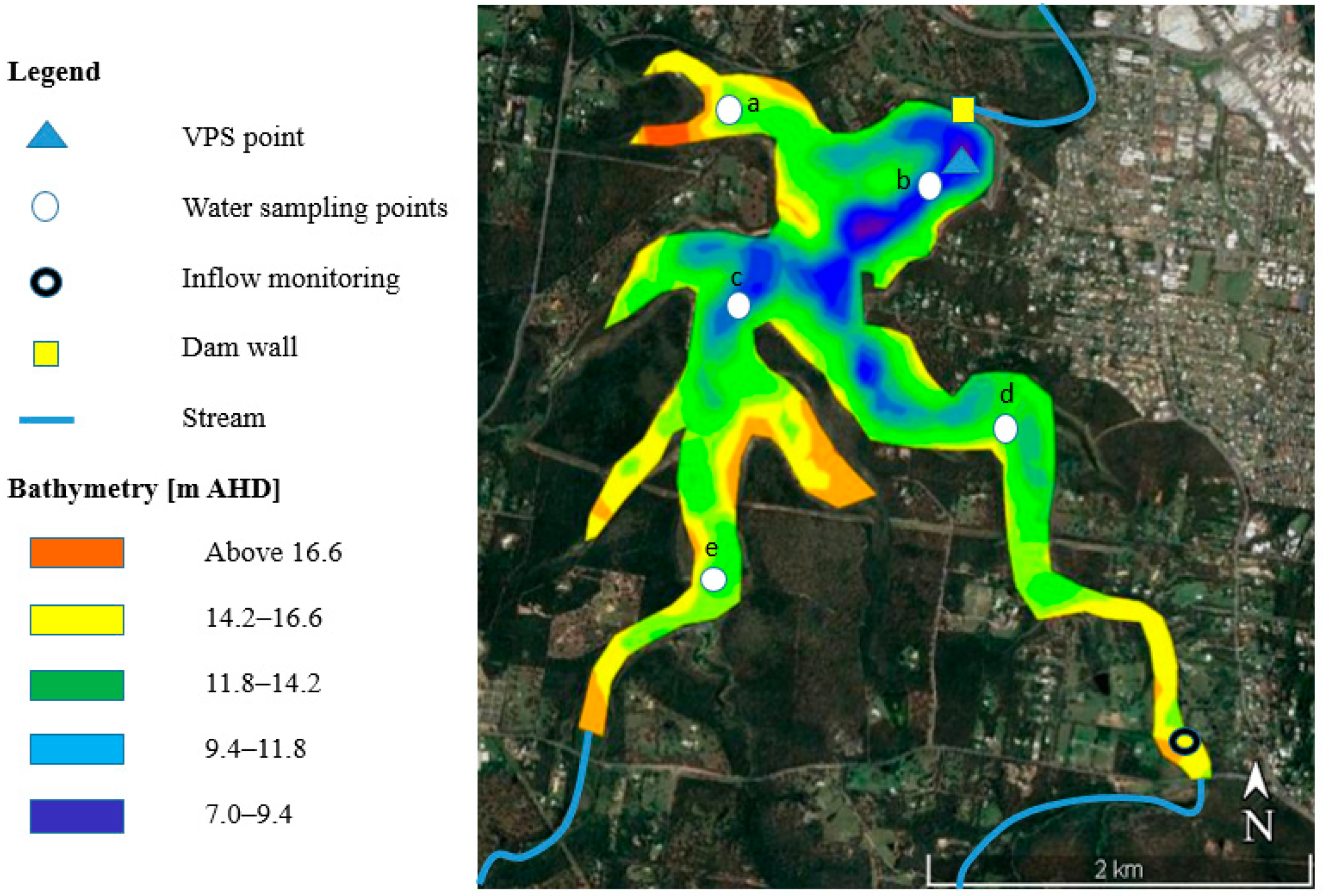
Tingalpa Reservoir is located in South-East Queensland, Australia (153.18° E, 27.53° S), and is bounded by Leslie Harrison Dam. The earth-fill dam structure, which was completed in 1968, is 25 m high and 535 m long. It was upgraded in 1984 to provide approximately 20% of the water supply to Redland City, which has a population of around 150,000 inhabitants. The shallow reservoir, with a mean depth of 5.3 m, has a mean water residence time of 4.5 years [26]. The main inflows are the Tingalpa Creek from a southwestern direction and the Stockyard Creek from a southeastern direction, see Figure 1. An intake tower, located on the northeastern side of the reservoir, withdraws the raw water and redirects it to the Capalaba water treatment plant (WTP). The catchment area is 87.5 square kilometers, and contains a large portion of the Venman Bushland National Park; the reservoir’s surface area at full capacity is 470 hectares. The dam was initially managed by the Redland City Council, but its management was transferred to Seqwater (i.e., Southeast Queensland Water) in July 2008. In order to ensure the region’s dams continue to meet national standards, Seqwater commenced dam improvement programs in 2014 and the dam’s capacity decreased from the full capacity (24,868 ML) to 13,206 ML on 1 August 2014. Previous studies [27] found that longer seasonally dry spells in Tingalpa Reservoir increased organic matter content, and affected water quality after the subsequent rainfall events.
2.2. Data Collection and Analysis
Since 2013, a VPS was installed in Tingalpa Reservoir 500 m from the dam wall, as shown in Figure 1. Such systems consist of a YSI (Yellow Springs, OH, USA) EXO2 multi-probe system connected to a set of water quality probes underneath, which are automatically winched up and down the water column and measure water quality variables, including water temperature, pH, dissolved oxygen, conductivity, turbidity and fDOM. In Tingalpa reservoir, the VPS can collect such water quality data for the full vertical profile every hour at 1-m depth intervals, and transmit the collected data via telemetry to the Seqwater dataset. The location where the VPS is placed has a maximum depth of 13 m. The fDOM was measured using an EXO2 fDOM Smart Sensor (YSI, USA) and reported as relative fluorescence units (RFU) and quinine sulfate units (QSU). This fDOM probe has an excitation/emission pair of 365 ± 5 nm/480 ± 40 nm to estimate the quantity of fluorescent, humic-like DOM (peak C) [28]. When monitoring the fDOM concentration, the optical signal of the fDOM probe is affected and distorted by temperature, turbidity, pH, salinity and inner filter effects. The type of turbidity is also important, with the magnitude of fDOM signal bias being related to the shape and size of suspended particles [29,30]. Sequential compensation models were recently developed to investigate such environmental interferences on a fDOM probe for its calibration in Tingalpa Reservoir [30]. Such models were applied to the raw fDOM historical data collected for this study, in order to achieve more reliable fDOM readings. In this study, the fDOM readings were compensated based on a recently developed sequential compensation model [31]. The uncompensated fDOM represents the original raw fDOM reading, which is affected by the aforementioned interferences.
For the determination of DOM concentrations, DOC and UV absorbance historical data from 2013 to 2017 were collected from Seqwater. These were originally measured from water samplings, following filtration. The sampling points are shown in Figure 1. DOC concentration was measured using a high-temperature catalytic oxidation TOC-L CPH Total Organic Carbon Analyser (Shimadzu Corporation, Japan). UV absorbance was measured using a UV-1800 UV-Visible Spectrophotometer (Shimadzu Corporation, Japan), with results given in cm−1. Specific absorbance or SUVA (the ratio of absorbance at 254 mm/m to DOC concentration) was determined at the raw water inlet. The time interval between water sampling was approximately one month. Historical weather conditions, such as air temperature, wind speed and direction, solar radiation and precipitation, were collected from the Australian Bureau of Meteorology (BoM) from 2013 to 2017 with a daily interval. Outflow discharge was obtained from Seqwater with a daily interval, including the outflow volume to the Capalaba Water Treatment Plant (WTP) and the spilt amount of water from Leslie Harrison Dam during a period from 2013 to 2017. Seqwater also monitored the daily inflow water level at the monitoring station shown in Figure 1 in Tingalpa Creek from 2014 to 2017.
The collected data for the 2013 to 2017 period was quality assured before being included in any data analysis to make sure the current results are reliable and reflect the dynamics observed in Tingalpa Reservoir. Thus, all data was checked for completeness, inconsistencies and anomalies. The collected dataset was checked for outliers and missing data. For the missing hourly VPS data, nearest-neighbours linear interpolation was performed, but for periods with longer gaps in data collection, (e.g., missing from 6 April 2015 to 5 May 2015), the interpolation was not implemented since it would be too unreliable. In this situation, when the vertical profiles are plotted in a time series format, unavailable data are shown in a white colour. Scatter plots of variables with each other helped to visually identify any linear or nonlinear correlation. All of these analyses enabled the understanding of the relationships between the physical and chemical variables and mixing processes in the reservoir.
3. Model Development
A one-dimensional model was developed to calculate the mixing coefficients using the VPS data, based on a continuity equation and an advection-diffusion equation. Regarding this vertical mixing model, water temperature and conductivity are the inputs for the boundary conditions. According to Bertone et al. [9], this model outputs the vertical velocity and diffusion coefficients, which can be used for analysing the mixing processes in lakes when VPS data is available.
When the inflow and outflow conditions are neglected, the differential equation for the conservation of mass can be derived from Equation (1) as:
where = density of water, = velocity vector and = gradient operator.
Equation (1) is also called the continuity equation. The continuity equation was discretized as follows:
where the superscript n is an index for time and subscript i is an index for depth (i = 1 indicates the bottom depth); and are the density of the water and the vertical velocity; is the lake cross area in the layer i, which is assumed to change with depth, but not over time; is the time step; is the distance between two adjacent depths. The water column was discretized with = 3600 s and = 1 m. The initial condition = 0, can be calculated using Equation (2). In the present study, the VPS collected water temperature and conductivity in the water column. The density can be calculated as in Millero and Poisson [32]:
where is the water density [kg/m3]; is the density of pure water [kg/m3], function of the water temperature; is the salinity of water [psu], which can be calculated by function of conductivity [33]; and are coefficients which are calculated by function of water temperature.
The advection-diffusion equation for heat transport is:
where is the water temperature at time and at depth z; is the reservoir cross area at depth ; is the vertical diffusion at time and at depth z; is the volumetric heat capacity of water; is the heat source term due to heat exchange with external environment, which is ignored in the present study.
The advection term in Equation (4) can be discretized as:
The diffusion term in Equation (4) can be discretized as:
Using Equations (5) and (6), the vertical velocity and the diffusion for each layer at each time can be calculated by applying all VPS data, in particular, water temperature and conductivity.
4. Results and Discussion
4.1. Analysis of Collected Data
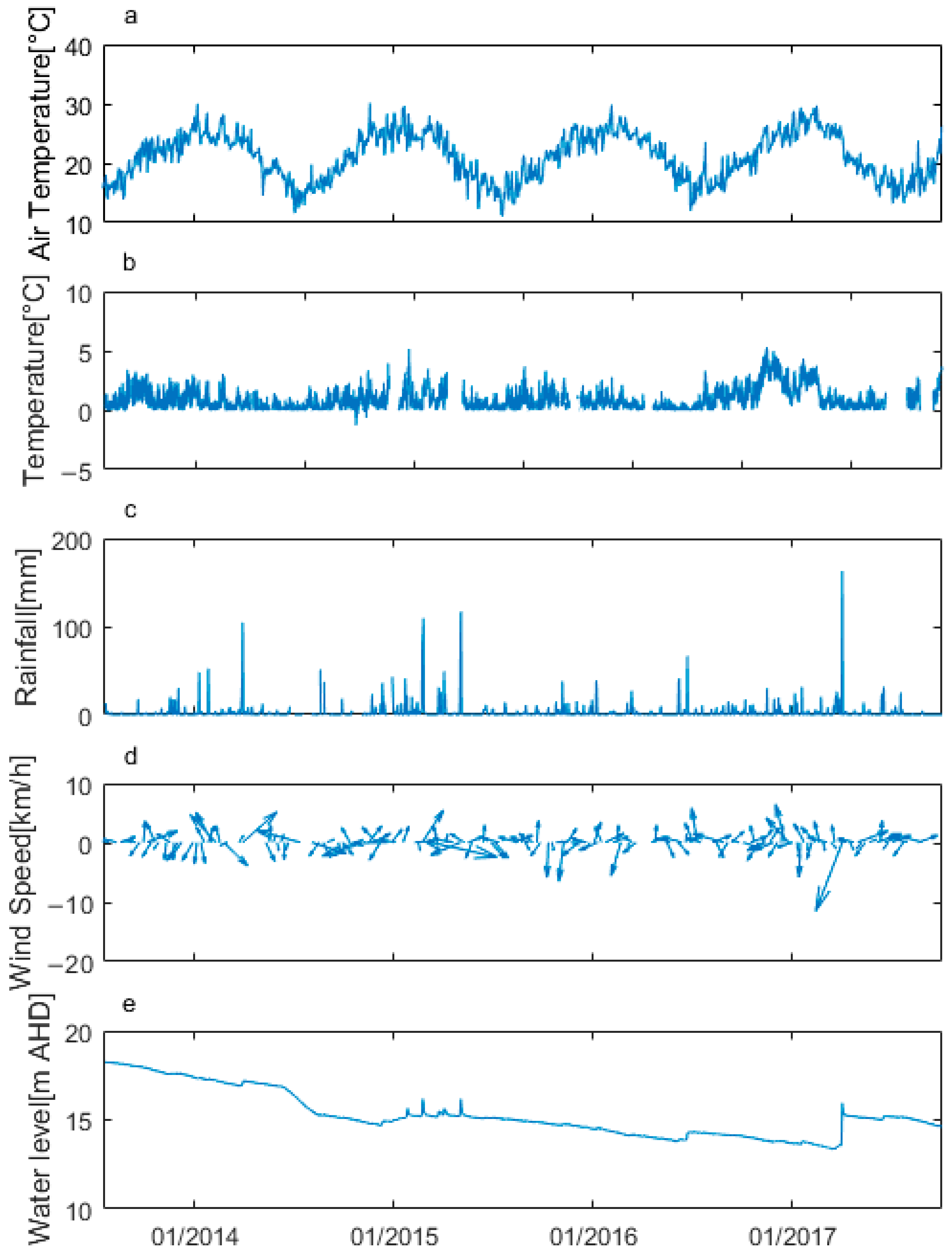
Daily averaged air temperature, the sum of daily rainfall, weekly wind condition (wind speed and wind direction), daily reservoir water level and hourly water temperature at depths of 1 m and 10 m and the column temperature differential are presented in Figure 2.
The air temperature varied seasonally within the range of 11.1–30.1 °C, with the highest air temperature from December to February (January is the warmest month with a monthly mean air temperature above 24.0 °C from 2014 to 2016) and the lowest in June to August (July is the coldest month with a monthly mean air temperature of 15.3 °C from 2014 to 2016). The monthly mean minimum and maximum temperatures for summer and winter months during the monitoring period were within the range of 24.1–26.9 °C and 14.6–17.2 °C, respectively. Thus, Tingalpa Reservoir is characterised by having a warm summer and mild winter which is consistent with its location (subtropical climate zone). In Figure 2a,b, the relationships are given between air temperatures and the column temperature differential, besides other variables. It illustrates that air temperature has larger fluctuation ranges than water temperature. For most of the summer seasons, the water temperature at the surface was higher than that of water at the bottom layers. However, when the air temperature decreased to the lowest value, the temperature in both layers of water reached the same level, thus achieving full thermal destratification.
During the period from July 2013 to July 2017, the precipitation distribution amongst seasons was 46.7% in summer, 21.7% in autumn, 20.0% in spring and 11.6% and winter. Heavy rainfall events caused by storms are most likely to occur during the summer months, see Figure 2c. The mean of the daily average of the wind speed and wind direction were 5.9 m s−1 and 145.9° (i.e., S/SE), respectively. The daily averaged wind speed varied between 0.8–18.3 m s−1 and the daily averaged wind direction varied between 36°–282.5°. To clearly show the wind variation, the wind condition with a weekly interval is plotted in Figure 2d. It is clear from the charts that heavy rainfall events were often associated with high wind speeds, and the dominant wind direction during storm events was NNW.
Figure 2e shows the water level variation during the monitoring period from 2013 to 2017 and presents a declining trend from highest level (18.1 m AHD) to lowest value (14.2 m AHD). It is obvious from the charts that heavy rainfall events lead to increases in the water level in Tingalpa Reservoir and decreases in the water temperature in both the surface and bottom layers.
4.2. Diurnal Variations of Thermal Stratification and Vertical Water Velocity in Summer and Winter Seasons
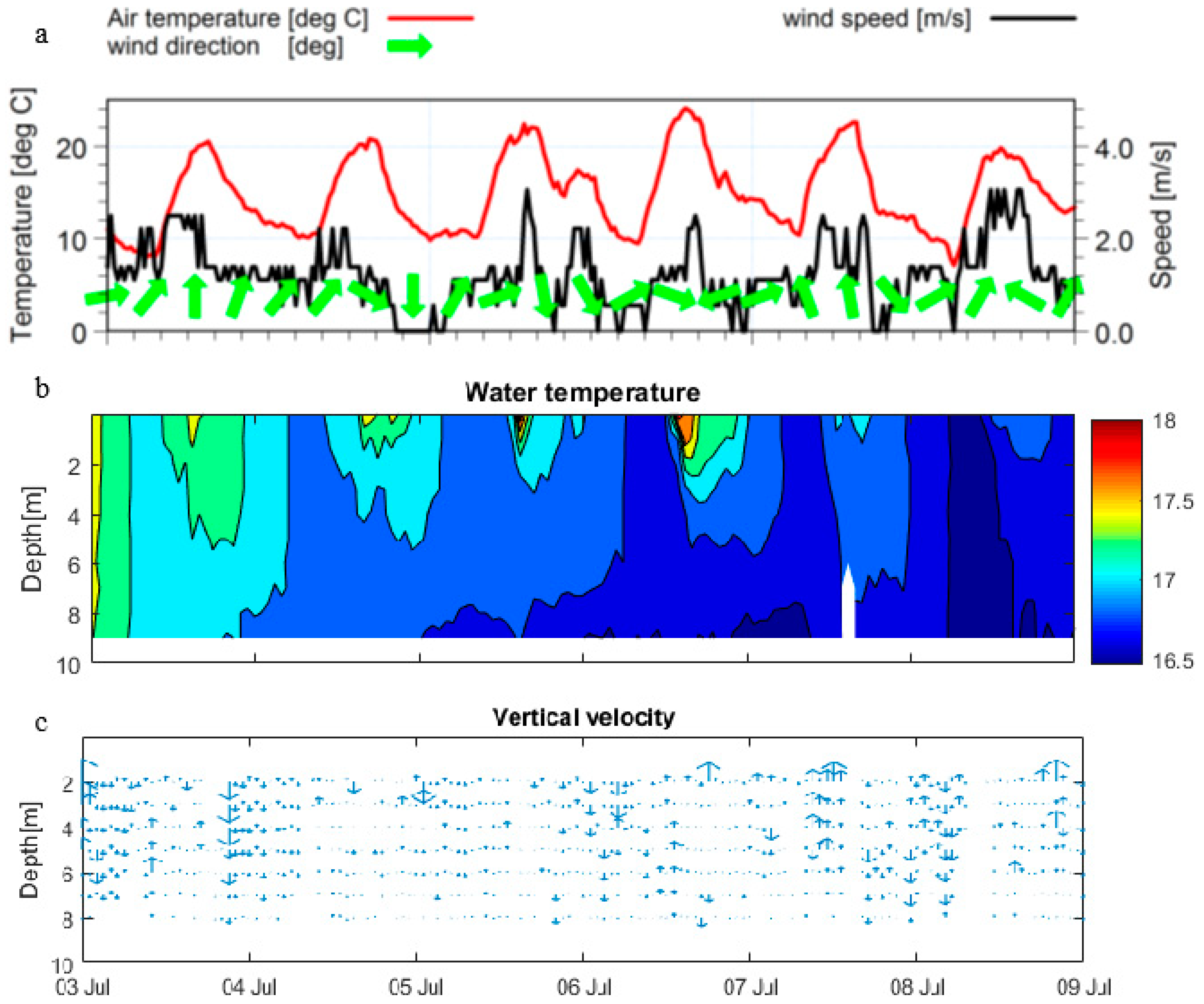
Vertical water velocity in winter from 3 July 2015 to 9 July 2015 was calculated using the 1D hydrodynamic model as shown in Figure 3c. It shows the diurnal mode in Tingalpa Reservoir and that the average vertical velocity values are in the order of 10−9 to 10−8 m/s. Figure 3 shows that the diurnal mode of vertical velocity, especially the top layers of water, is dominated by the force of the wind in winter (e.g., 3–9 July 2015). During this period, diurnal variations of thermal stratification were typical in winter. Figure 3a,b show the air and water temperature and wind conditions. The results of the vector plot of vertical velocity indicate that high wind speeds contribute to an increase of vertical velocity in the surface of the water, leading to destratification and water mixing in the water column. During the selected period (3–9 July 2015), the wind speed was generally relatively low (less than 2 m s−1) during night and early morning, except the night of 6 July 2015. The wind condition shows that from 7 July to 9 July 2015, prolonged strong winds persisted and removed heat, contributing to fewer changes of the water temperature gradients during this period. The wind speed peaked when air temperature increased to the maximum value around 11 AM to 3 PM. The water temperature profile (Figure 3b) showed the thermal stratification in the day time gradually declined and there was very little stratification over these last two days. The thermal gradients occurred when air temperature increased and relatively large gradients were limited to the top 4m. The wind blowing at night led to destratification in the top layers of water.
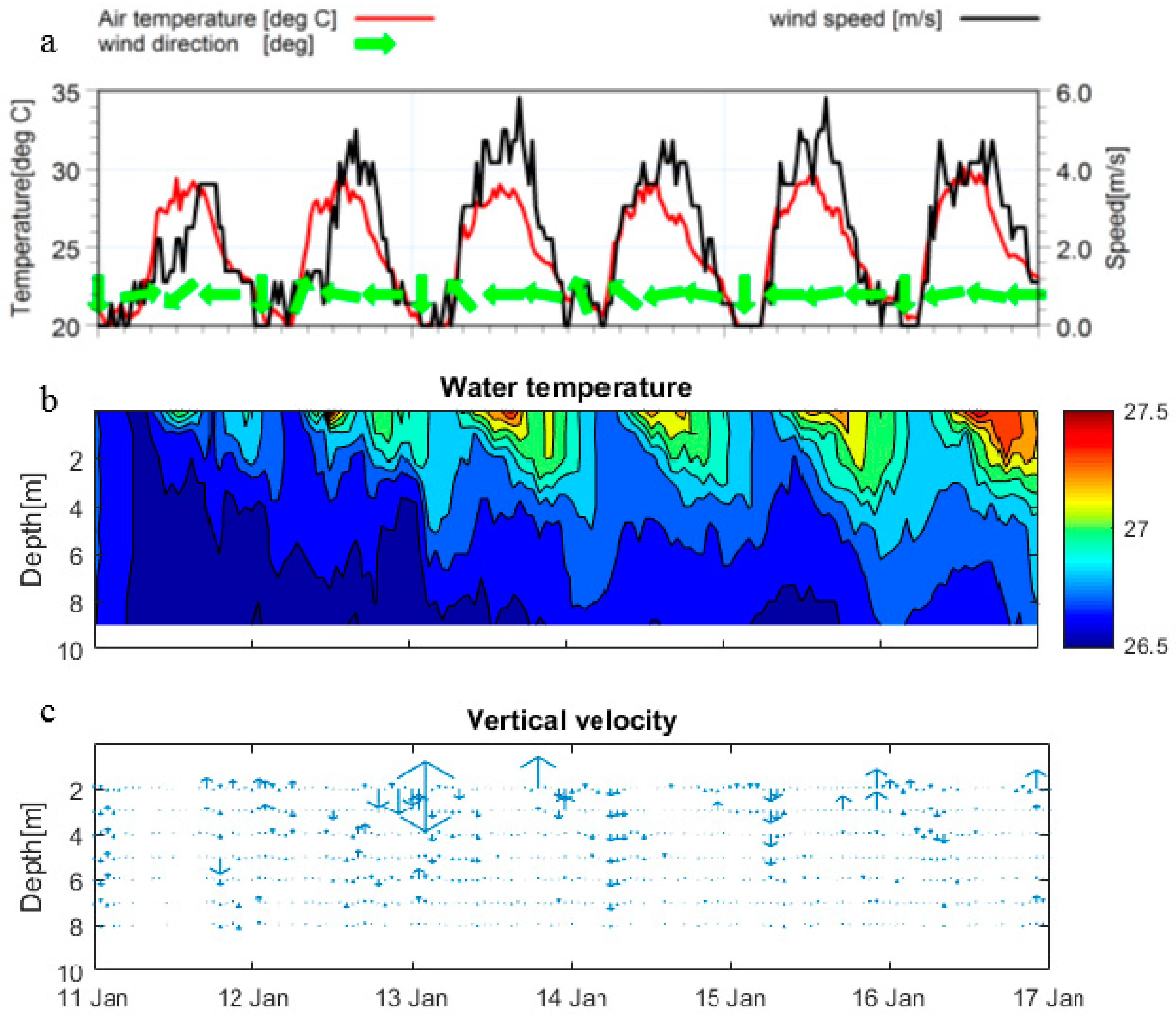
The vertical water velocity, as well as the water temperature, in summer from 11 Jan 2014 to 17 Jan 2014 are presented in Figure 4. The air temperature and wind conditions are also presented in Figure 4. The range of water temperatures (26.5 °C to 27.5 °C) was less than that of air temperatures (20 °C to 30 °C). Regarding the wind condition, the figure indicated that during this period, the wind speed was generally low at midnight and increased in the daytime. Low-speed wind was from a northern or southern direction and the relatively high-speed wind was from an easterly direction. The diurnal regimes over these six days were similar. The surface water started to heat between 9 AM to 11 AM and the thermal stratification extended into the night. Although a prolonged easterly wind blew, the thermal gradients were preserved within the top 4 m through to the night.
Overall, higher thermal gradients occur at the top layers of water (limited to 6 m). The prolonged wind cannot influence the progress of the water temperature being heated in summer. However, in winter, the strong wind contributes to water mixing and destratification in the water column. In Tingalpa Reservoir, due to the shallow reservoir depth, thermal stratification cannot continue for a long time and water is always mixed in the vertical direction at night. It seems feasible to develop a model that, given the existing thermal stratification and air temperature, predicts the minimum wind speed and direction necessary to fully destratify the reservoir.
4.3. Seasonal Variation of DOM Concentration and Compositions
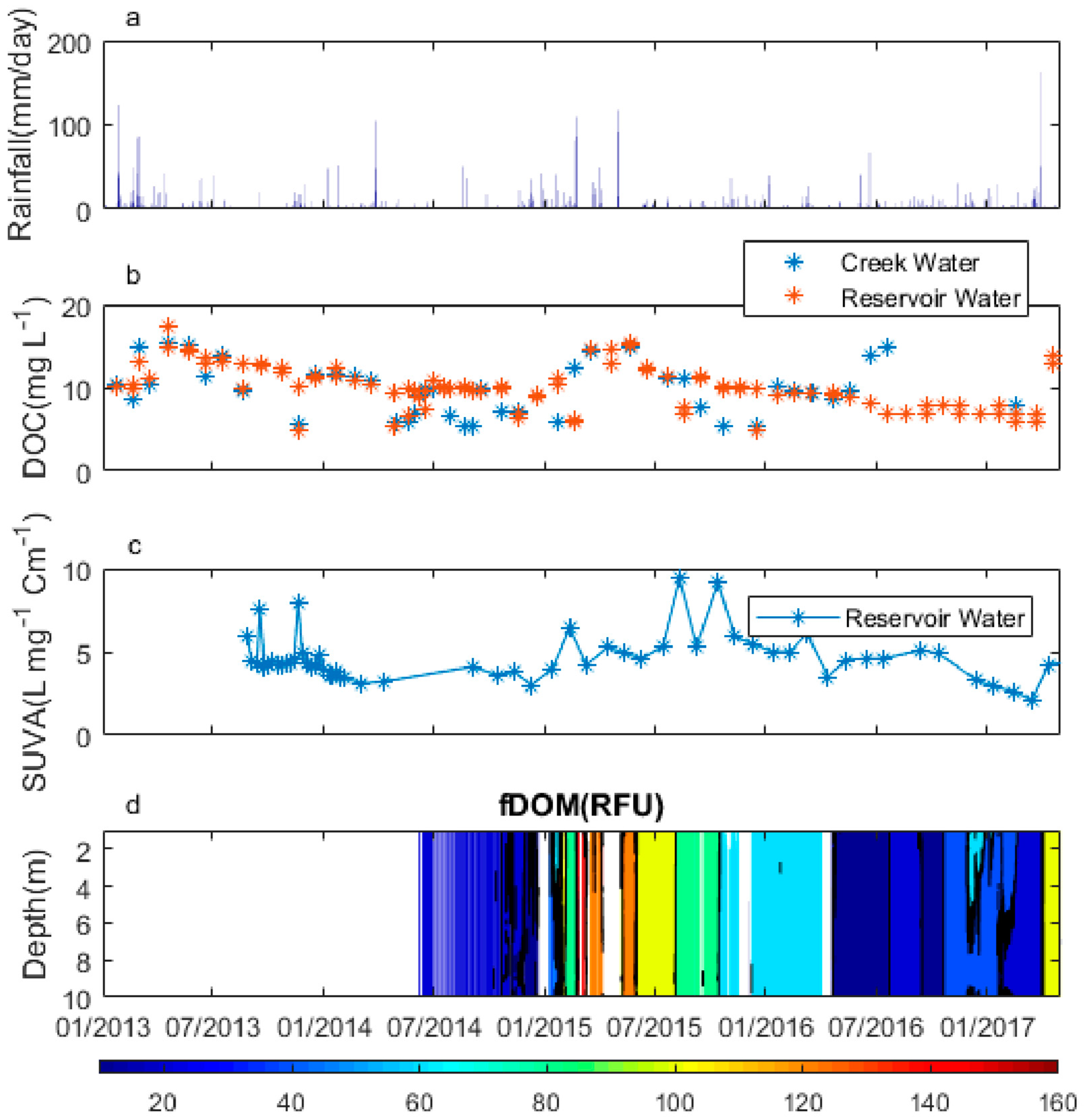
The concentrations of DOC in Tingalpa Creek and the reservoir are shown in Figure 5b. It shows there is a clear correlation between DOC and rainfall intensity. Heavy rainfall led to the highest DOC concentrations (monthly mean value: 14.3 mg/L) occurring in the wet period (March–May) in 2015. This parameter showed a similar trend in 2013 and 2015, with a peak in the wet period in 2013 (mean value of 13.93 mg/L). The peak value always occurred in the wet period, which agrees with the findings from Evans et al. [34] and Saraceno et al. [35]. They reported that the DOM concentration increased in stream waters during storm events.
DOC concentrations in reservoir waters in 2013, 2014 and 2015 showed a similar seasonal variation trend to that in river waters, decreasing in dry periods and increasing in the wet period in Figure 5b. In contrast, this parameter had a different trend to river waters in 2016, especially the period from July to August 2016. DOC concentrations increased from 10.2 mg/L to 15.6 mg/L in Tingalpa Creek. However, DOC concentrations decreased from 9.18 mg/L to 7.4 mg/L in reservoir waters. The different variations can be attributed to a longer residence time in Tingalpa Reservoir in this period (mean 23.2 days). Compared to a smaller residence time (mean 0.2 days) in spring 2015, a longer residence time can help to dilute the DOC concentrations.
Figure 5c shows that SUVA values were less than 5 L mg-C−1 m−1 in most of the seasons. Mean SUVA levels in the reservoir waters were lower in summer than other seasons, especially in 2016. In 2016, the mean SUVA value was 2.93 L mg-C−1 m−1 in summer and mean SUVA values were higher than 4 L mg-C−1 m−1 in other seasons in this year, which means that reservoir water contains hydrophobic, high molecular-weight aromatic humic substances [36]. The difference in SUVA levels between summer season and other seasons was statistically significant (p-value = 0.0053). This variation is due to increasing UV irradiation levels from spring to summer, leading to coloured aromatic DOM being degraded by sunlight [37]. Figure 5d indicates that the fDOM had a similar variation trend to that of the DOC concentration in reservoir water, i.e., an increase from July 2014 to April 2015 and a decline after April 2015.
4.4. Effects of Extreme Events in Mixing Processes
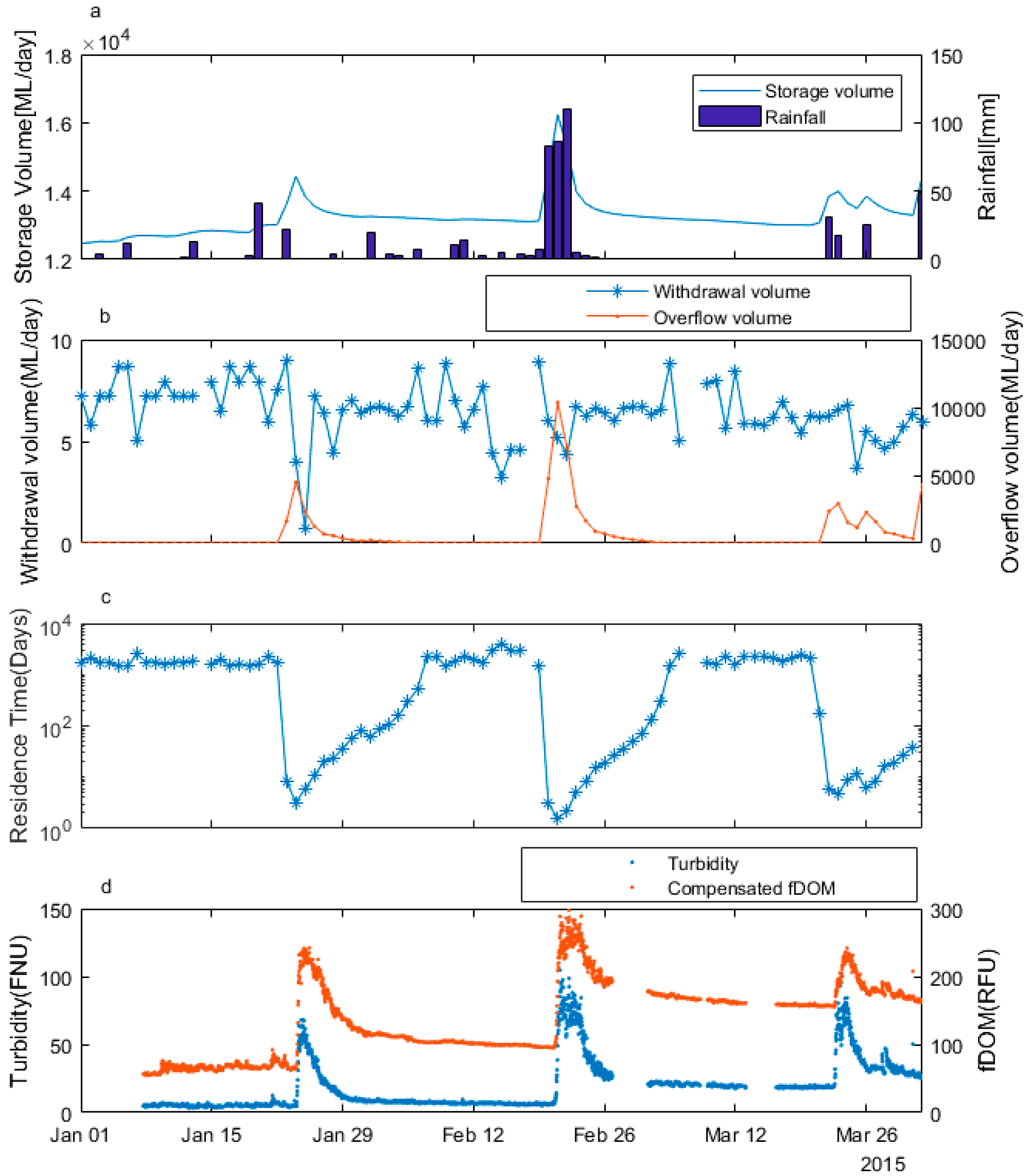
The rainfall, the storage volume and the outflow which comprises water withdrawal and overflow via the spillway are presented in Figure 6 together with the water quality (turbidity and compensated fDOM) variations in Tingalpa Reservoir.
During the period 1 January 2015 to 1 April 2015, three heavy storm events occurred and caused increases in the storage volume. The average water withdrawal is approximately 6.45 ML d−1 and varied between 0.7–8.98 ML d−1. The overflow over the spillway varied in accordance with the storage volume, specifically between 0–10,370 ML d−1. Based on the ratio between the storage volume of the reservoir and the total outflow, the variation in the hydraulic residence time was estimated, see Figure 6c. The hydraulic residence time represents the average length of time that water resides in a reservoir, which significantly influences water quality [38]. The results show that the residence time in Tingalpa Reservoir decreased from approximately 17,000 days to five days during these extreme events. It is obvious that the short residence time led to increases in turbidity and compensated fDOM. Four storm events generated between 2015 and 2017 were selected, see Table 1. The duration of turbidity is defined as the time period from the start of rainfall to the time when turbidity varied less than 5%/hour; it can be seen in Table 1 that the duration of extreme events exceeded 100 h; for Event 3, the duration of the turbidity event was only 57 h. The reason for a shorter time for storm event 3 is that it is closer to the time of storm event 2. After event 2, the reservoir was still recovering and had a short response time to storm event 3. The lag time of each parameter is relative to the time of the peak rainfall. Lastly, it should be noted that these four events follow the reduction in the dam’s capacity. Therefore, decreasing dam level and heavy rainfall are the two significant factors causing not only very high turbidity levels, but long event durations. There was no obvious post-rainfall variation in the turbidity levels before decreasing the dam level. In fact, previous studies [39] showed a two-fold increase in the average raw water turbidity following the approximately 50% reduction in storage volume for Tingalpa reservoir. These results suggest that before decreasing dam levels, Tingalpa reservoir had enough volume to dilute the turbidity inflows so that no significant impact on the water quality was observed. Event 2 and Event 4 experienced intense rainfall, so the following paragraphs focus on these two events.
4.4.1. Storm Event 2—Cyclone Marcia
Severe tropical Cyclone Marcia crossed Southeast Queensland and was accompanied by heavy rainfall from 20 February to 22 February 2015. Figure 7 shows the effects of such rainfall events on the reservoir’s water quality.
In situ turbidity at the bottom layer increased from 6.78 NTU to the peak value of 104.75 NTU in 15 hours between 20 and 21 February, 2015. Turbidity at the depth of 10 m returned to a stable value (40 NTU) after 3 days. Comparing the turbidity levels at other depths, the variation in the level of the water at the bottom was more dramatic. However, the turbidity level in different layers returned to the same value after this event. The water temperature in each layer decreased rapidly during the heavy rainfall, and the decreasing rate in the deeper layers (2.66 °C /day) was higher than that in surface water (1.07 °C /day). After the heavy rainfall, the surface water temperature exhibited diurnal variability, but the temperature in the bottom layers didn’t have such diurnal variation. The fDOM response to Cyclone Marcia resulted in a large increase in fDOM values in the vertical direction and differences in the magnitude of changes in both compensated and original fDOM concentrations. Compensated fDOM at the depth of 10 m reached the peak value (280 RFU) on 22 February. Uncompensated fDOM at the depths of 1 m and 10 m and compensated fDOM at a depth of 1 m increased between 21 and 24 February and remained stable after 24 February. The range of compensated fDOM (90 RFU–280 RFU) was significantly larger than that of uncompensated fDOM (90 RFU–140 RFU), thus highlighting the importance of appropriately adjusting the sensors’ readings for interferences to allow for robust, reliable measurement. Before the storm event 2, the average vertical velocity in the water column was in the order of 10−9 to 10−8 m/s and the diffusivity values were in the range of 10−5–10−3 m2/s. During storm event 2, the vertical velocity and diffusivity increased up to 10−7 m/s and 0.08 m2/s, respectively, and the value of both vertical velocity and diffusivity were larger at the surface layer of water. This implies the storm event enabled short-term vertical water mixing and promoted surface waters sinking down towards deeper layers.
4.4.2. Storm Event 4—Cyclone Debbie
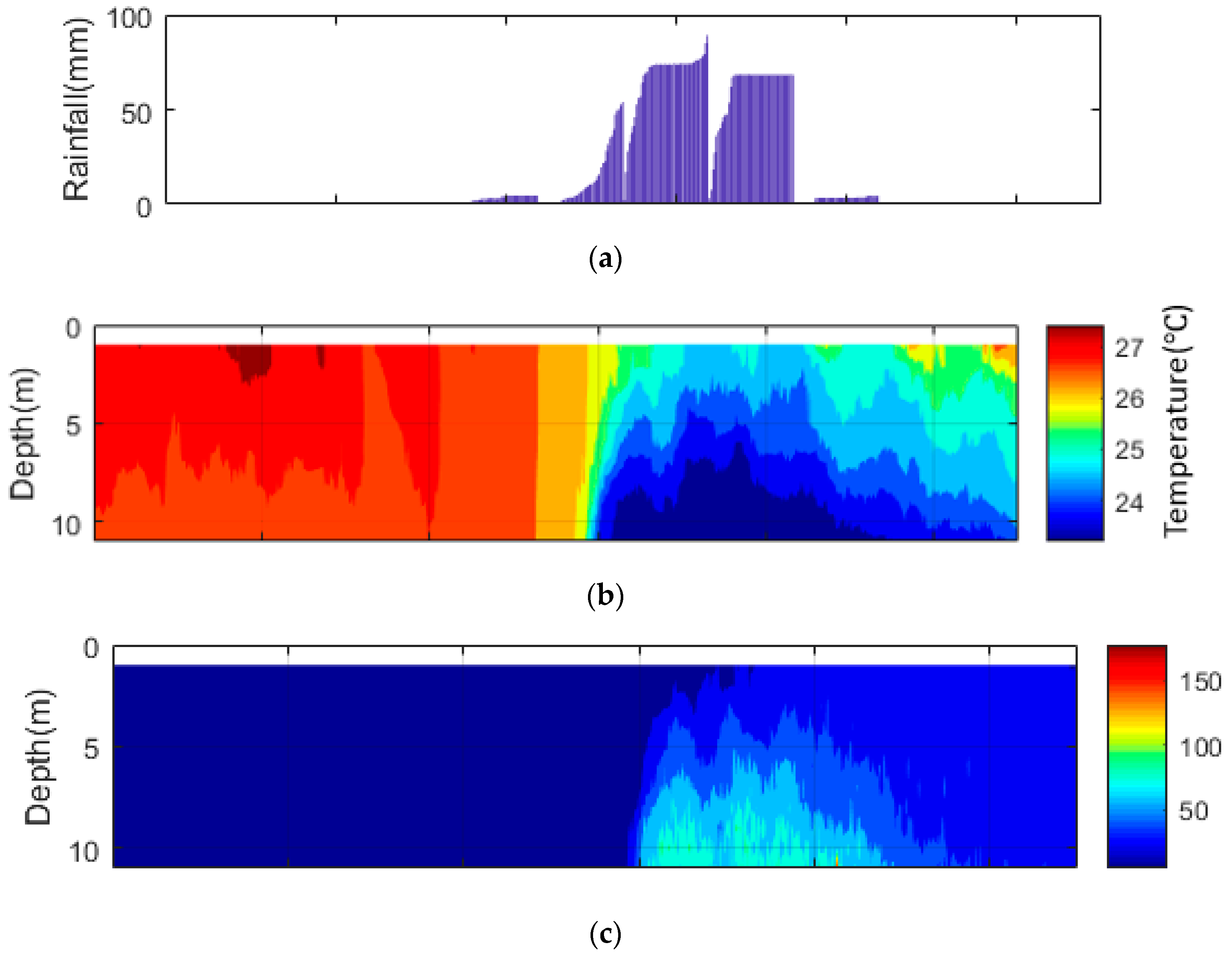
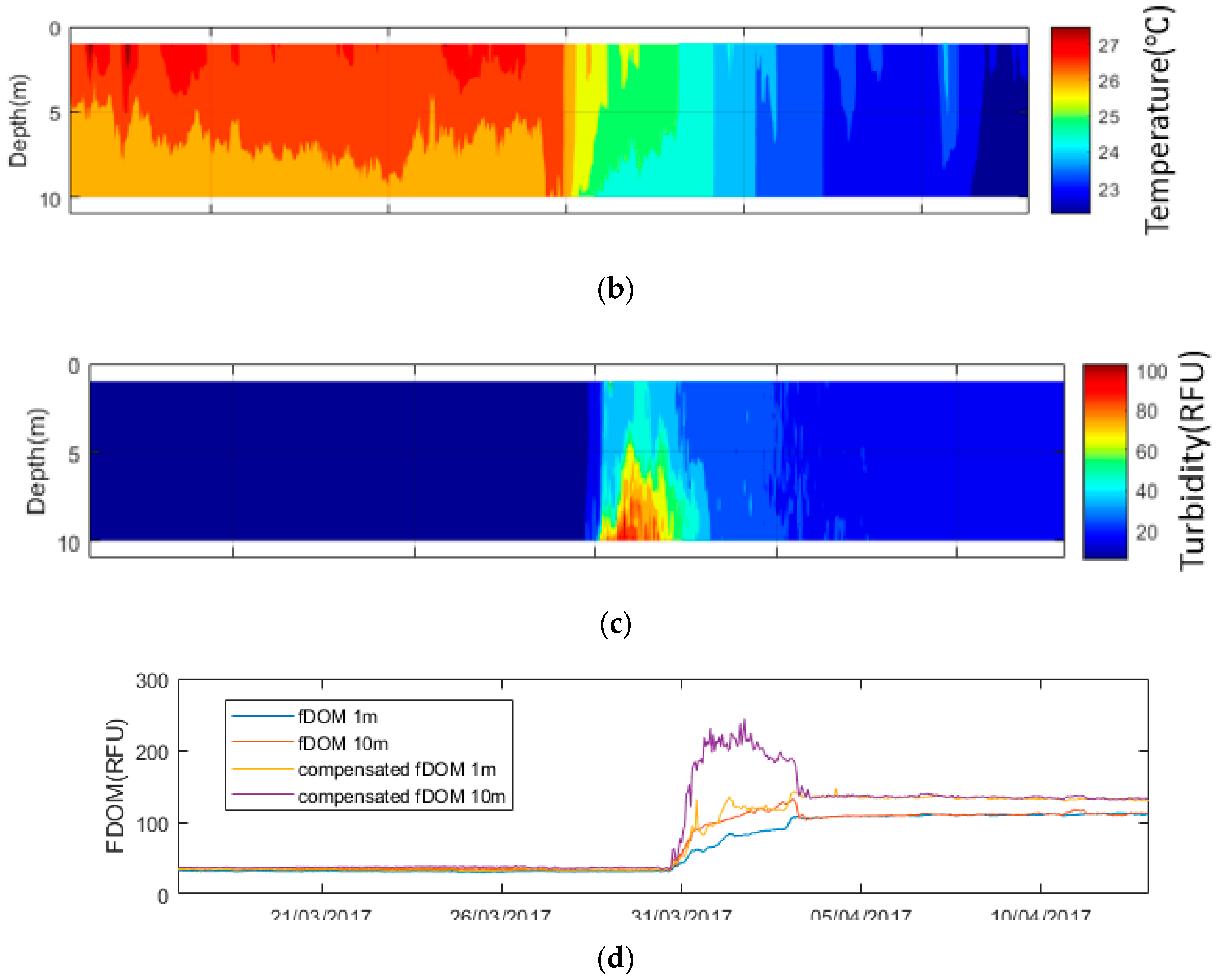
Ex-tropical cyclone Debbie impacted over Tingalpa Reservoir during the afternoon and evening of Thursday, 30th March 2017. Damaging wind gusts of up to 131 km/h were observed along with widespread rainfall in excess of 150 mm. Figure 8 shows the impact of such an event on the reservoir’s water quality.
In situ turbidity increased during the heavy rainfall and the turbidity level at the bottom layer was higher than that of the top layers. The turbidity level in different layers returned to the same value (22 NTU) four days after this event. The water temperature in each layer decreased rapidly during the heavy rainfall from 26 °C to 22.5 °C. The temperature had diurnal variabilities before and after the heavy rainfall, but this diurnal fluctuation decreased during the storm event. It is a similar behaviour to that for storm event 2, where the peak values of vertical velocity and diffusivity were in the range of 10−2 m/s and 10−7 m2/s, respectively.
During ex-tropical cyclone Debbie, there were many differences between compensated fDOM and uncompensated fDOM between the top and bottom layers of the water. Compared to compensated fDOM at the depth of 1 m, uncompensated fDOM in this layer increased more uniformly from 32 RFU to 110 RFU. The compensated fDOM concentration at the depth of 10 m reached the peak of 230 RFU on 1 April, which is less than the peak value during Cyclone Marcia. It is noted that both compensated and uncompensated fDOM decreased sharply on 3 April and the decrease continued for 7 h. After 4 April, the fDOM concentration remained in a stable state. In addition, compared to deeper layers, near-surface waters seem to be affected to a much lower extent in terms of poor water quality (turbidity and compensated fDOM), hence the highest offtake would provide a reasonable option. However, depending on the circumstances, such as a more extreme event mixing the whole column and lower water level, it shows that, typically, the water quality would recover in only a few days, hence if other resources are accessible, water managers may choose withdraw a small amount of water from Tingalpa Reservoir for a few days.
5. Conclusions
The mixing processes in Tingalpa reservoir, Queensland, Australia have been investigated in this study using, among others, high-frequency VPS data. A one-dimensional model was developed and implemented for analysing the vertical mixing of waters in Tingalpa Reservoir.
Heavy rainfall events accompanied by higher wind speeds, which were significant in summer seasons, led to increases in the water level in Tingalpa Reservoir and decreases of water temperature in both the surface and bottom layers. When the water level remained stable and there was little rainfall, a prolonged thermal stratification occurred. The DOC concentration both in reservoir water and inflow river water always peaked in wet periods and decreased in dry seasons. The longer residence time in Tingalpa Reservoir can provide enough time to dilute the DOC concentration in reservoir water. For the diurnal thermal stratification in Tingalpa Reservoir, most of the stratification is restricted to the upper layers of water in both summer and winter in the absence of precipitation. The duration of thermal gradients within the top meters is longer in summer than in winter, and often persists until the early morning in summer, while in winter, night winds are able to break it down. The implemented vertical mixing model, which is based on vertical profiles of water temperature and conductivity collected from the VPS, can be applied in real time to calculate the vertical velocity and diffusivities. The model enables a better understanding of mixing processes affecting the reservoir and adds value to the VPS instrumentation.
For the water quality data analysis, the lag time between peaks in turbidity and compensated fDOM relative to the rainfall event was between 17 to 20 h during a number of analysed storm events. The VPS data in each storm event showed that before decreasing the dam level, Tingalpa Reservoir had enough dilution capacity to keep turbidity and DOM levels to much lower levels. However, after lowering the dam level, storm events led to much higher increases in turbidity and fDOM.
This study provides useful insights into the effects of extreme weather events on mixing processes and water quality of shallow sub-tropical reservoirs. Specifically, for Tingalpa Reservior, it provides insights to water managers on how storm events impact water quality, including at which depths and for how long. Future work will focus on the development of a fDOM-based hybrid (data-driven and process-based) decision support tool for the Capalaba water treatment plant, able to simulate the effects of extreme weather events (e.g., heavy storms, drought) on reservoir DOM concentration, thus assisting with its removal.
Author Contributions
Conceptualization, H.Z., E.B. and R.A.S.; methodology, X.W. and H.Z.; software, X.W.; validation, X.W. and E.B.; formal analysis, X.W.; data curation, K.O.; writing—original draft preparation, X.W.; writing—review and editing, H.Z., E.B., R.A.S. and K.O.
Funding
This research was partially funded by the Australian Government through the Australian Research Council (ARC LP160100217).
Acknowledgments
This research work was conducted with the technical and financial support of Seqwater and Griffith University.
Conflicts of Interest
The authors declare no conflict of interest.
References
- Elçi, Ş. Effects of thermal stratification and mixing on reservoir water quality. Limnology 2008, 9, 135–142. [Google Scholar] [CrossRef]
- MacIntyre, R. Oxygen depletion in Lake Macquarie, NSW. Mar. Freshw. Res. 1968, 19, 53–56. [Google Scholar] [CrossRef]
- MacKinnon, M.; Herbert, B. Temperature, dissolved oxygen and stratification in a tropical reservoir, Lake Tinaroo, northern Queensland, Australia. Mar. Freshw. Res. 1996, 47, 937–949. [Google Scholar] [CrossRef]
- Boehrer, B.; Schultze, M. Stratification of lakes. Rev. Geophys. 2008, 46. [Google Scholar] [CrossRef]
- Weider, L.J.; Lampert, W. Differential response of Daphnia genotypes to oxygen stress: Respiration rates, hemoglobin content and low-oxygen tolerance. Oecologia 1985, 65, 487–491. [Google Scholar] [CrossRef]
- Seager, J.; Milne, I.; Mallett, M.; Sims, I. Effects of short-term oxygen depletion on fish. Environ. Toxicol. Chem. 2000, 19, 2937–2942. [Google Scholar] [CrossRef]
- Marsden, M.W. Lake restoration by reducing external phosphorus loading: The influence of sediment phosphorus release. Freshw. Biol. 1989, 21, 139–162. [Google Scholar] [CrossRef]
- Søndergaard, M.; Jensen, J.P.; Jeppesen, E. Role of sediment and internal loading of phosphorus in shallow lakes. Hydrobiologia 2003, 506, 135–145. [Google Scholar] [CrossRef]
- Bertone, E.; Stewart, R.A.; Zhang, H.; O’Halloran, K. Analysis of the mixing processes in the subtropical Advancetown Lake, Australia. J. Hydrol. 2015, 522, 67–79. [Google Scholar] [CrossRef]
- Zhang, H.; Chan, E.-S. Modeling of the turbulence in the water column under breaking wind waves. J. Oceanogr. 2003, 59, 331–341. [Google Scholar] [CrossRef]
- Townsend, S.A. The influence of retention time and wind exposure on stratification and mixing in two tropical Australian reservoirs. Archiv für Hydrobiologie 1998, 141, 353–371. [Google Scholar] [CrossRef]
- Dorjsuren, B.; Yan, D.; Wang, H.; Chonokhuu, S.; Enkhbold, A.; Yiran, X.; Girma, A.; Gedefaw, M.; Abiyu, A. Observed Trends of Climate and River Discharge in Mongolia’s Selenga Sub-Basin of the Lake Baikal Basin. Water 2018, 10, 1436. [Google Scholar] [CrossRef]
- Wilhelm, S.; Adrian, R. Impact of summer warming on the thermal characteristics of a polymictic lake and consequences for oxygen, nutrients and phytoplankton. Freshw. Biol. 2008, 53, 226–237. [Google Scholar] [CrossRef]
- Holland, A.; Stauber, J.; Wood, C.M.; Trenfield, M.; Jolley, D.F. Dissolved organic matter signatures vary between naturally acidic, circumneutral and groundwater-fed freshwaters in Australia. Water Res. 2018, 137, 184–192. [Google Scholar] [CrossRef] [PubMed]
- Stedmon, C.A.; Markager, S.; Bro, R. Tracing dissolved organic matter in aquatic environments using a new approach to fluorescence spectroscopy. Mar. Chem. 2003, 82, 239–254. [Google Scholar] [CrossRef]
- Tundisi, J.G.; Tundisi, T.M. Limnology; CRC Press: Boca Raton, FL, USA, 2012. [Google Scholar]
- Weithoff, G.; Lorke, A.; Walz, N. Effects of water-column mixing on bacteria, phytoplankton, and rotifers under different levels of herbivory in a shallow eutrophic lake. Oecologia 2000, 125, 91–100. [Google Scholar] [CrossRef]
- Wiedner, C.; Nixdorf, B.; Heinze, R.; Wirsing, B.; Neumann, U.; Weckesser, J. Regulation of cyanobacteria and microcystin dynamics in polymictic shallow lakes. Archiv für Hydrobiologie-Hauptbände 2002, 155, 383–400. [Google Scholar] [CrossRef]
- Judd, K.; Adams, H.; Bosch, N.; Kostrzewski, J.; Scott, C.; Schultz, B.; Wang, D.; Kling, G. A case history: Effects of mixing regime on nutrient dynamics and community structure in Third Sister Lake, Michigan during late winter and early spring 2003. Lake Reserv. Manag. 2005, 21, 316–329. [Google Scholar] [CrossRef]
- Helfer, F.; Zhang, H.; Lemckert, C. Modelling of lake mixing induced by air-bubble plumes and the effects on evaporation. J. Hydrol. 2011, 406, 182–198. [Google Scholar] [CrossRef]
- Blix, K.; Pálffy, K.; Tóth, V.R.; Eltoft, T. Remote Sensing of Water Quality Parameters over Lake Balaton by Using Sentinel-3 OLCI. Water 2018, 10, 1428. [Google Scholar] [CrossRef]
- Toming, K.; Kutser, T.; Tuvikene, L.; Viik, M.; Nõges, T. Dissolved organic carbon and its potential predictors in eutrophic lakes. Water Res. 2016, 102, 32–40. [Google Scholar] [CrossRef] [PubMed]
- Hood, E.; Gooseff, M.N.; Johnson, S.L. Changes in the character of stream water dissolved organic carbon during flushing in three small watersheds, Oregon. J. Geophys. Res. Biogeosci. 2006, 111. [Google Scholar] [CrossRef]
- Spencer, R.G.; Aiken, G.R.; Butler, K.D.; Dornblaser, M.M.; Striegl, R.G.; Hernes, P.J. Utilizing chromophoric dissolved organic matter measurements to derive export and reactivity of dissolved organic carbon exported to the Arctic Ocean: A case study of the Yukon River, Alaska. Geophys. Res. Lett. 2009, 36. [Google Scholar] [CrossRef]
- Ruhala, S.S.; Zarnetske, J.P. Using in-situ optical sensors to study dissolved organic carbon dynamics of streams and watersheds: A review. Sci. Total Environ. 2017, 575, 713–723. [Google Scholar] [CrossRef] [PubMed]
- Burford, M.A.; Johnson, S.A.; Cook, A.J.; Packer, T.V.; Taylor, B.M.; Townsley, E.R. Correlations between watershed and reservoir characteristics, and algal blooms in subtropical reservoirs. Water Res. 2007, 41, 4105–4114. [Google Scholar] [CrossRef] [PubMed]
- Lu, J.; Faggotter, S.J.; Bunn, S.E.; Burford, M.A. Macrophyte beds in a subtropical reservoir shifted from a nutrient sink to a source after drying then rewetting. Freshw. Biol. 2017, 62, 854–867. [Google Scholar] [CrossRef]
- Coble, P.G. Characterization of marine and terrestrial DOM in seawater using excitation-emission matrix spectroscopy. Mar. Chem. 1996, 51, 325–346. [Google Scholar] [CrossRef]
- Saraceno, J.F.; Shanley, J.B.; Downing, B.D.; Pellerin, B.A. Clearing the waters: Evaluating the need for site-specific field fluorescence corrections based on turbidity measurements. Limnol. Oceanogr. Methods 2017, 15, 408–416. [Google Scholar] [CrossRef]
- De Oliveira, G.; Bertone, E.; Stewart, R.; Awad, J.; Holland, A.; O’Halloran, K.; Bird, S. Multi-Parameter Compensation Method for Accurate In Situ Fluorescent Dissolved Organic Matter Monitoring and Properties Characterization. Water 2018, 10, 1146. [Google Scholar] [CrossRef]
- Oliveira, G.; Bertone, E.; Stewart, R.; O’Halloran, K. Understanding and modelling fluorescent dissolved organic matter probe readings for improved coagulation performance in water treatment plants. In Proceedings of the 22nd International Congress on Modelling and Simulation, Hobart, Australia, 3–8 December 2017. [Google Scholar]
- Millero, F.J.; Poisson, A. International one-atmosphere equation of state of seawater. Deep Sea Res. Part A Oceanogr. Res. Pap. 1981, 28, 625–629. [Google Scholar] [CrossRef]
- American Public Health Association. Standard Methods for the Examination of Water and Wastewater; American Public Health Association: Washington, DC, USA, 1989. [Google Scholar]
- Evans, C.D.; Monteith, D.T.; Cooper, D.M. Long-term increases in surface water dissolved organic carbon: Observations, possible causes and environmental impacts. Environ. Pollut. 2005, 137, 55–71. [Google Scholar] [CrossRef] [PubMed]
- Saraceno, J.F.; Pellerin, B.A.; Downing, B.D.; Boss, E.; Bachand, P.A.; Bergamaschi, B.A. High-frequency in situ optical measurements during a storm event: Assessing relationships between dissolved organic matter, sediment concentrations, and hydrologic processes. J. Geophys. Res. Biogeosci. 2009, 114. [Google Scholar] [CrossRef]
- Van Nieuwenhuijzen, A.; Van der Graaf, J. Handbook on Particle Separation Processes; IWA Publishing: London, UK, 2011. [Google Scholar]
- Awad, J.; van Leeuwen, J.; Chow, C.; Drikas, M.; Smernik, R.J.; Chittleborough, D.J.; Bestland, E. Characterization of dissolved organic matter for prediction of trihalomethane formation potential in surface and sub-surface waters. J. Hazard. Mater. 2016, 308, 430–439. [Google Scholar] [CrossRef] [PubMed]
- Ji, Z.-G. Hydrodynamics and Water Quality: Modeling Rivers, Lakes, and Estuaries; John Wiley & Sons: Hoboken, NJ, USA, 2017. [Google Scholar]
- Bertone, E.; O’Halloran, K. Analysis and Modelling of Taste and Odour Events in a Shallow Subtropical Reservoir. Environments 2016, 3, 22. [Google Scholar] [CrossRef]
Figure 1.
Monitoring sites in Tingalpa Reservoir. In the background, the bathymetry [m AHD] of Tingalpa Reservoir is presented.
Figure 1.
Monitoring sites in Tingalpa Reservoir. In the background, the bathymetry [m AHD] of Tingalpa Reservoir is presented.

Figure 2.
Time series of: (a) Daily air temperature; (b) hourly column water temperature differential between depths of 1 m and 10 m; (c) daily rainfall; (d) weekly wind condition and (e) daily water level in Tingalpa Reservoir from 2013 to 2017.
Figure 2.
Time series of: (a) Daily air temperature; (b) hourly column water temperature differential between depths of 1 m and 10 m; (c) daily rainfall; (d) weekly wind condition and (e) daily water level in Tingalpa Reservoir from 2013 to 2017.

Figure 3.
Time series of (a) air temperature and wind conditions; (b) the vertical profile of water temperature; (c) vector plot vertical velocity for the top 9 m in winter from 3 July 2015 to 9 July 2015 for Tingalpa Reservoir.
Figure 3.
Time series of (a) air temperature and wind conditions; (b) the vertical profile of water temperature; (c) vector plot vertical velocity for the top 9 m in winter from 3 July 2015 to 9 July 2015 for Tingalpa Reservoir.

Figure 4.
Time series of (a) air temperature and wind conditions; (b) the vertical profile of water temperature; (c) vector plot vertical velocity for the top 9 m in summer from 11 Jan 2014 to 17 Jan 2014 for Tingalpa Reservoir.
Figure 4.
Time series of (a) air temperature and wind conditions; (b) the vertical profile of water temperature; (c) vector plot vertical velocity for the top 9 m in summer from 11 Jan 2014 to 17 Jan 2014 for Tingalpa Reservoir.

Figure 5.
Time series of (a) daily precipitation, (b) monthly DOC concentration in creek water and reservoir water (station b), (c) monthly SUVA in reservoir water and (d) hourly fDOM concentration (unit: RFU), 2013–2017 for Tingalpa Reservoir.
Figure 5.
Time series of (a) daily precipitation, (b) monthly DOC concentration in creek water and reservoir water (station b), (c) monthly SUVA in reservoir water and (d) hourly fDOM concentration (unit: RFU), 2013–2017 for Tingalpa Reservoir.

Figure 6.
(a) Daily rainfall (mm d−1) and daily storage volume (ML), (b) outflow (withdrawal and overflow via spillway) (ML d−1), (c) residence time (Days), (d) hourly turbidity (FNU) and compensated fDOM (RFU) at the depth of 10 m for the period 1 January 2015 to 1 April 2015 for Tingalpa Reservoir.

Figure 7.
Precipitation and ancillary in situ VPS from 15 February to 26 February 2015 including (a) half hourly rainfall (mm·d−1), (b) hourly temperature (°C), (c) hourly turbidity (FNU), (d) hourly original fDOM and compensated fDOM (RFU) at the depths of 1 m and 10 m in storm event 2.
Figure 7.
Precipitation and ancillary in situ VPS from 15 February to 26 February 2015 including (a) half hourly rainfall (mm·d−1), (b) hourly temperature (°C), (c) hourly turbidity (FNU), (d) hourly original fDOM and compensated fDOM (RFU) at the depths of 1 m and 10 m in storm event 2.


Figure 8.
Precipitation and ancillary in situ VPS from 15 February to 26 February 2015 including (a) half hourly rainfall (mm·d−1), (b) hourly temperature (°C), (c) hourly turbidity (FNU), (d) hourly original fDOM and compensated fDOM (RFU) at the depths of 1 m and 10 m in storm event 4.
Figure 8.
Precipitation and ancillary in situ VPS from 15 February to 26 February 2015 including (a) half hourly rainfall (mm·d−1), (b) hourly temperature (°C), (c) hourly turbidity (FNU), (d) hourly original fDOM and compensated fDOM (RFU) at the depths of 1 m and 10 m in storm event 4.


Table 1.
Relevant parameters in Tingalpa Reservoir in extreme events.
| Parameter | Event 1 | Event 2 | Event 3 | Event 4 |
|---|---|---|---|---|
| Time period | 19/01/2015–29/01/2015 | 20/02/2015–26/02/2015 | 22/03/2015–27/03/2015 | 30/03/2017–03/04/2017 |
| Total Rainfall (mm) | 66.6 | 288.8 | 74.4 | 214 |
| Storm duration (Hour) | 96 | 70 | 47 | 48 |
| Duration of turbidity (Hour) | 103 | 117 | 57 | 103 |
| Max turbidity (FNU) | 67.87 | 104.75 | 92.90 | 111.90 |
| Lag time of turbidity (Hour) | 17 | 16 | 18 | 20 |
| Average increasing rate of turbidity (FNU/hour) | 9.8 | 7.22 | 5.59 | 3.87 |
| Max compensated fDOM | 242.13 | 297.86 | 241.95 | 244.38 |
| Lag time compensated fDOM (Hour) | 17 | 16 | 18 | 20 |
© 2019 by the authors. Licensee MDPI, Basel, Switzerland. This article is an open access article distributed under the terms and conditions of the Creative Commons Attribution (CC BY) license (http://creativecommons.org/licenses/by/4.0/).
Share and Cite
MDPI and ACS Style
Wang, X.; Zhang, H.; Bertone, E.; Stewart, R.A.; O’Halloran, K. Analysis of the Mixing Processes in a Shallow Subtropical Reservoir and Their Effects on Dissolved Organic Matter. Water 2019, 11, 737. https://doi.org/10.3390/w11040737
AMA Style
Wang X, Zhang H, Bertone E, Stewart RA, O’Halloran K. Analysis of the Mixing Processes in a Shallow Subtropical Reservoir and Their Effects on Dissolved Organic Matter. Water. 2019; 11(4):737. https://doi.org/10.3390/w11040737
Chicago/Turabian StyleWang, Xinchen, Hong Zhang, Edoardo Bertone, Rodney A. Stewart, and Kelvin O’Halloran. 2019. "Analysis of the Mixing Processes in a Shallow Subtropical Reservoir and Their Effects on Dissolved Organic Matter" Water 11, no. 4: 737. https://doi.org/10.3390/w11040737
Note that from the first issue of 2016, this journal uses article numbers instead of page numbers. See further details here.