Identification of the Most Suitable Probability Distribution Models for Maximum, Minimum, and Mean Streamflow


1
School of Environmental and Rural Science, University New England, Armidale, NSW 2351, Australia
2
Central Queensland University, School of Health, Medical and Applied Sciences, Bundaberg Campus, University Drive, Bundaberg, QLD 4670, Australia
*
Author to whom correspondence should be addressed.
Water 2019, 11(4), 734; https://doi.org/10.3390/w11040734
Submission received: 22 February 2019
/
Revised: 4 April 2019
/
Accepted: 5 April 2019
/
Published: 9 April 2019
(This article belongs to the Section Hydrology)
Abstract
:Hydrological studies are useful in designing, planning, and managing water resources, infrastructure, and ecosystems. Probability distribution models are applied in extreme flood analysis, drought investigations, reservoir volumes studies, and time-series modelling, among other various hydrological studies. However, the selection of the most suitable probability distribution and associated parameter estimation procedure, as a fundamental step in flood frequency analysis, has remained the most difficult task for many researchers and water practitioners. This paper explains the current approaches that are used to identify the probability distribution functions that are best suited for the estimation of maximum, minimum, and mean streamflows. Then, it compares the performance of six probability distributions, and illustrates four fitting tests, evaluation procedures, and selection procedures through using a river basin as a case study. An assemblage of the latest computer statistical packages in an integrated development environment for the R programming language was applied. Maximum likelihood estimation (MLE), goodness-of-fit (GoF) tests-based analysis, and information criteria-based selection procedures were used to identify the most suitable distribution models. The results showed that the gamma (Pearson type 3) and lognormal distribution models were the best-fit functions for maximum streamflows, since they had the lowest Akaike Information Criterion values of 1083 and 1081, and Bayesian Information Criterion (BIC) values corresponding to 1087 and 1086, respectively. The Weibull, GEV, and Gumbel functions were the best-fit functions for the annual minimum flows of the Tana River, while the lognormal and GEV distribution functions the best-fit functions for the annual mean flows of the Tana River. The choices of the selected distribution functions may be used for forecasting hydrologic events and detecting the inherent stochastic characteristics of the hydrologic variables for predictions in the Tana River Basin. This paper also provides a significant contribution to the current understanding of predicting extreme hydrological events for various purposes. It indicates a direction for hydro-meteorological scientists within the current debate surrounding whether to use historical data and trend estimation techniques for predicting future events with issues of non-stationarity and underlying stochastic processes.
1. Introduction
Rivers and floodplains are important components of any country’s economic, social, and cultural development. However, extreme streamflows and flood changes in magnitude and frequency may have disastrous effects on humans, riparian communities, and the environment in river basins [1,2,3]. Water systems infrastructure for hydropower, water supply, and irrigation, as well as human life and settlement and riparian ecosystems, are often affected by these flood and drought phenomena. Real-time flood forecasting [4] and the construction of large structures can help mitigate flood and drought hazards and minimise their related losses, but the danger of these natural hazards due to their very extreme probability of occurrence cannot be completely avoided, and water engineers often face major challenges in estimating the frequency of these rare events for a site or region [5,6]. One major problem faced by water engineers is the determination of the most suitable form of an extreme value model, the underlying probability distribution of the flood, and the approximation of parameters of the distribution. Specifying the frequency of occurrence of the possible values of a random variable through probability distribution is of immense importance for the planning, engineering design, and management of water systems and hydraulic structures, including drought hazards, urban planning, growth forecasting [7], agrosystem management, and environment ecosystem management in river basins.
Many techniques are available for flood analysis using historical data, such as for instance the traditional flood frequency approach [8], mixed-population graphical approach, and statistical models. Hydrologic events are highly stochastic in nature; therefore, extremal flood discharge distribution determination by the statistical fitting of probability distributions to the historical recorded extremal discharge data can be effective compared to the deterministic and physical-based traditional methods [9,10]. The use of probabilistic approaches to fit and select the best fitting probability model to a set of observed data has lately gained currency among researchers [11]. A number of probability distribution models viz., Weibull, gamma (Pearson type 3), generalised extreme value (GEV), lognormal, Gumbel, and normal are in use in the hydrologic frequency analysis of floods [12,13]. The choice of a model follows a procedure with a number of steps, starting with the critical analysis of historical data, the selection of an event-descriptive variable to examine the magnitude of a flood, and finally, evaluating the adequacy between a flood sample and a distribution type to inform the selection. The selection of a "best fit’ probability distribution and its parameter estimation procedure has remained an active and challenging research area [14,15]. Accurate predictions of the magnitude and frequency of flood flows and water drought occurrences are necessary for the planning, design, and operation of irrigation water use and water control projects, floodplain zonation and management, and ecosystem and agro-system management. Floods, flooding, and water droughts (low flows) are common problems in many river basins in tropical developing countries where river flows are critical for livelihood support systems. Therefore, it is important that uniform flood and drought frequency methods for the development of national flood and disaster management programs [16]) are considered in these countries. This will also allow facilitation and proper coordination among government agencies and line ministries as well as the private sector, farmers, and pastoral communities that participate in the management of river basin water resource systems that are affected by flood and water drought risks. Guidelines for flood frequency distribution models used in the design and planning of infrastructure, such as for example the guidelines provided in Bulletin 17B that are being used in the United States [17], have been developed through the use of probability distributions. Historical streamflow data are observed over a long period of time in a river system and are analysed in frequency analysis to relate the magnitude of extreme events of floods or water droughts to their frequency of occurrence. However, the use of historical data and present estimation techniques in flood frequency analysis have raised concerns regarding the adequacy for reasoning and deduction in hydrological modelling with issues of hydro-meteorological non-stationarity and the stochastic nature of hydrologic events [15]. Such concerns and the need for accurate deductions in hydrological modelling require a basis for discussions [18].
The aim of this study is to review the flood frequency analysis methods and illustrate their application in selecting the best flood frequency models for fitting hydrological streamflow extremes. The objective is to provide an overview of the methods with an illustration in the case study, and hence serve as a basis for future debates in hydrological modelling under a changing climate and the non-stationarity of stochastic processes. In Section 2 of this paper, a synthesis of the common steps in statistical inference approaches currently in use in flood frequency analysis is presented, and a typical procedure and prior studies and recommendations from various parts of the world are also included. The study site and data, theoretical description of one of the most commonly used approaches, and best-fit selection and method used are provided in Section 3. Section 4 of the paper is devoted to the results of the case study; here, a comparison of the performance of six probability distributions and an illustration of the fitting test, evaluation, and selection procedures for identifying the best distribution suited for the estimation of extreme hydrological events for the Tana River Basin (TRB) in Kenya is presented. A discussion with a focus on the case study is given in Section 5, and the conclusions drawn from the study are finally presented in Section 6. This study provides important information for hydrological modelling and helps eliminate the application of an arbitrary use of the model distribution function. This work is of interest to hydrologists, designers of hydraulic structures, irrigation engineers, environmental managers, and planners of water resources.
2. Basic Steps in the Identification of Probability Distribution Models
The application of a probability model for hydrological extreme event modelling in any region or country for any specific purpose depends on the characteristics of available discharge data at a site [6,19]. Long-term discharge records of observations are generally preferred, and therefore, problems related to local flow conditions that vary over time, as well as the incompleteness and inconsistency of the data series, have to be considered through the screening and critical analysis of these records as a first step.
The second step is event sample variable selection to rate the magnitude of an extreme flood depending on the specific objectives of the investigation. Maximum flows are related to engineering flood risks, water systems infrastructure, and developing flood response strategies, whereas mean and minimum streamflow flood frequencies are important for understanding the hydrological drought, monitoring the environmental flows, irrigation, and agriculture, and managing ecosystems and natural resources. The frequency analysis of low flows is used to determine whether an irrigation scheme needs storage or not, and for planning and designing such storage if required. However, low-flow frequency analysis has not received as much attention as maximum flows in recent years [20], despite its relevance in regions where both peak floods and droughts have almost equal devastating effects. The selected flood may be applied as a whole sample or measured sequential sample series using block maxima or peaks over threshold sampling strategies [21]. The next step is selecting a mathematical function for the cumulative distribution from a number of probability distribution models.
The final step of the analysis involves the estimation of the parameter values’ distribution or distributions selected, and the identification of the best distribution model suited for the estimation of extreme hydrological events. There are many methods for the estimation of time-dependent hydroclimatic flood parameters. Here, we only discuss the most common and major ones. The method of moments (MOM) estimates population parameters by taking known facts about the population sample as the first moment condition and extending the same concepts to derive higher moments. Moments such as the skewness (s), coefficient of variations (σ2), kurtosis (k), expected moment (µ), and the parameters (θ) are presumed to be related to a distribution function—ó = g(μ, α2, s, k)—and are considered members of the underlying distribution (û, ŝ, ǩ, ᾅ) for providing parameters ô = g ((û, ŝ, ǩ, ᾅ) [21]. This method has the advantages of being simple to derive, consistent in providing estimators for continuous function, and providing starting estimates in search of maximum likelihood values. However, the estimators may not be unique in a given dataset, and thus can provide multiple solutions to a set of equations; furthermore, sometimes parameter estimates may suffer from inaccurate and insufficient statistics, especially for smaller population sizes.
L-moments techniques [22] have the advantages of not being affected by sampling variability as they are linear functions of the data sample and, unlike ordinary product moments, they are less subject to bias, because they avoid squaring sample estimators such as the variance and skew coefficient and cubing the observations [23,24]. The downside is that theoretically, they are more suited to small sample sizes and three-parameter distribution [25]. Furthermore, outliers can substantially influence these methods [26]. LH moments are generalised L-moments with the added ability of a more detailed analysis of characterising the upper part of distributions and larger flood events [27]. With this improvement, LH moments provide more efficiency for high-quantile estimation and the reduced effects of small sample events associated with the comparison to L moments. However, LH moments are more suited to the quantiles of the higher return periods, and they are out-performed by L moments when it comes to shorter return periods [28].
The expected moments algorithm (EMA) is another moments-based iteration algorithm developed from iterated least squares (ILS) method for fitting regression models to censored data in flood frequency analysis [29]. The iteration process starts with initial sample parameter estimates calculated using systematic flood gauge records; then, the parameters are updated using the previously estimated sample moments to obtain new moment estimators of the below-threshold floods. Although this method can be more efficient, it has the disadvantage of censoring low outliers in flood frequency data [30]. The other method is probability-weighted moments (PWMs) [31], which is closely related to L moments, but estimates parameters based on the probability-weighted moments approach. PWMs are often considered to be superior to standard moment-based estimates and may be useful in the absence of maximum likelihood estimates or if they are difficult to compute. The Bayesian method applies prior knowledge arising from an analysis of regional flood data to infer the posterior probability density of the parameters for the at-site flood records [32,33]. The demerits of the Bayesian method lie in the complexity of its implementation and its intensive computational requirements. However, with advancements in technology, it may become a useful non-stationarity flood frequency analysis model in the future [34]. Another approach is the probability density evolution method (PEDM) developed from probability-weighted moments [31]. Its advantages are that it circumvents the linear limitations in flood frequency analysis that are often encountered in parametric methods and avoids the problem of selecting the kernel function and window width in some nonparametric approaches [35]. However, its use in flood frequency analysis is still limited. The other procedural approach is the maximum likelihood estimation, which is one of the most theoretically sound and extensively used methods for fitting probability distributions to hydrological data [36]. This parameter estimation method starts with a mathematical equation called the likelihood function with unknown model parameters. The model values that maximise the sample likelihood become the maximum likelihood estimates (MLEs). Although this method can be heavily biased and require specialised computer software for solving complex non-linear mathematical functions, its advantages make it the most desirable approach given today’s availability of statistical packages to manage the MLE analysis.
We chose MLE (a theoretical description is given in Section 3.2) for parameter determination in this case study because of its desirable properties, which include its efficiency in using historical hydrological records and computational power [37,38]; these traits are not easily and/or are not well addressed by the L-moment estimation method [39] and the method of moments (MOM) [40]. Optimal properties and the very general and flexible framework of MLE makes it the most preferred method of parameter estimation.
There are many ways of modelling discrimination procedures in flood frequency analysis that are commonly referred to as goodness-of-fits (GoFs) [41,42]. Some of these are described in Section 3 of this paper. Recent research studies have used this approach to find suitable site-specific distributions, for example: Ndetei, Opere [12] recommended Gumbel distribution and generalised extreme value (GEV) for flood frequency analysis on Lake Victoria Basin rivers in Kenya. Others are Griffis and Stedinger [43], who suggested the log-Pearson 3, as recommended by Bulletin 17B, for streamflow modelling in the United States, and Rahman, Rahman [44], whose research found that log-Pearson 3, generalised extreme value, and generalised Pareto distributions are the best-fit distributions for most of the areas in the states of Australia. Pearson type 3, GEV, and lognormal models have been shown to provide a good approximation to flood-flow data in the southwestern United States [45]. Application of a probability model for hydrological extreme event modelling in any region or country for any specific purpose depends on the characteristics of available data at a site [6,19].
3. Study Site, Theoretical Descriptions, and Method
3.1. Study Site and Data
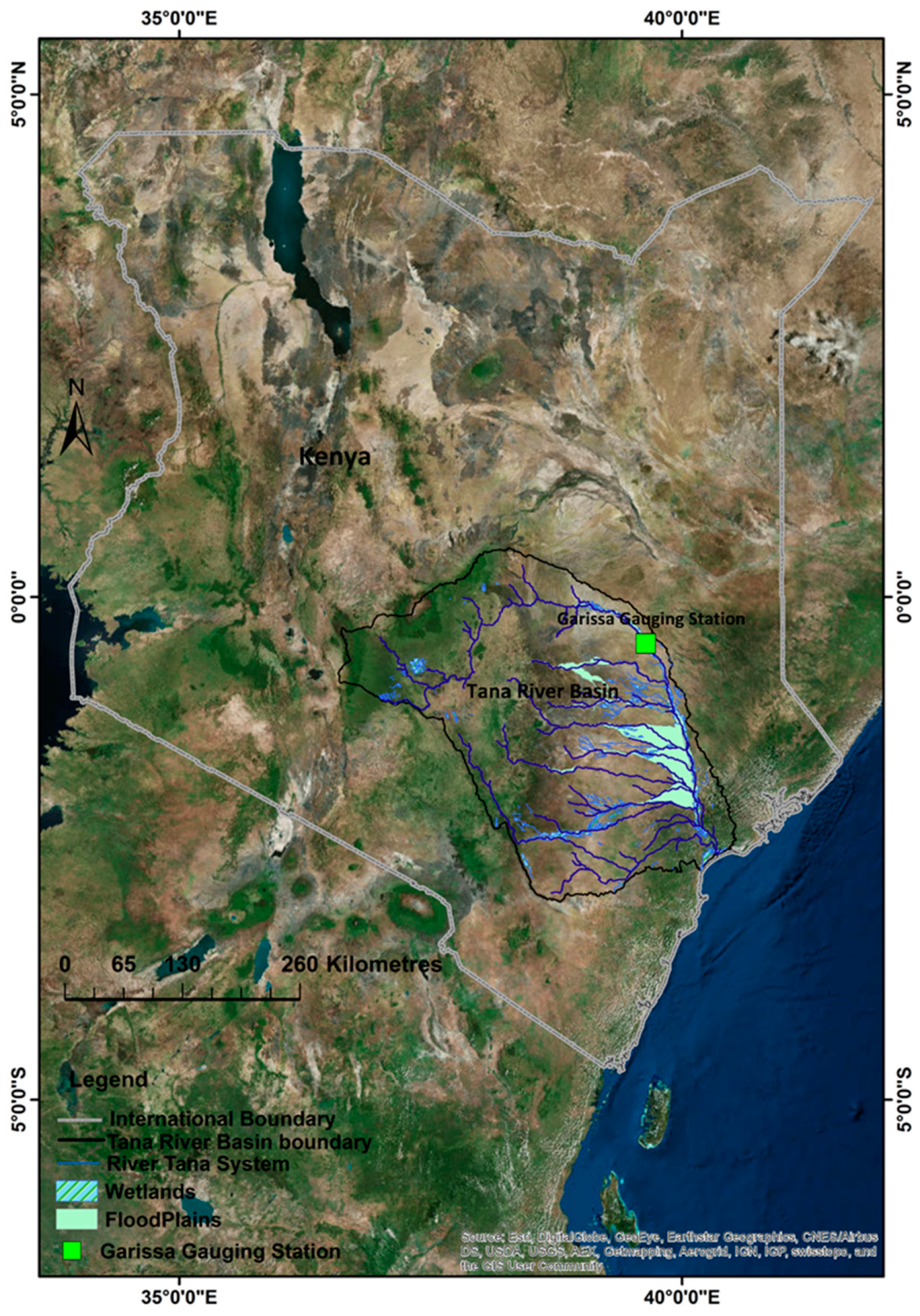
Tana River (Figure 1) is Kenya’s longest and largest river, and is of immense significance to the country’s economy, as well as both the upstream and downstream communities. Within the Tana River Basin (TRB), there are ambitious plans for water resources development, including multipurpose dams for hydropower generation and irrigation, as well as industrial and domestic water supply; expanding irrigation schemes; and inter and intra transfer diversions [46,47]. The Garissa discharge gauging station is located at 0°27′49.19″ S, 39°38′11.77″ E and has arguably the longest and most reliable streamflow observation records in the country; thus, it is the obvious reference for the planning, engineering design, and management of the proposed water systems in the basin. Kenya’s worst floods, which were attributed to Indian Ocean atmospheric circulation and surface temperatures, were recorded between 1961–1962 and 1997–1998 [48]. The later event created huge economic and social disruption due to its widespread, rapid, and prolonged flood [49] in Lower Tana. Damages caused by flood and drought disasters are expected to increase in the future within this basin, particularly at the Tana floodplain [50], which hosts large irrigation schemes, important biodiversity, and wetland areas of international importance. Therefore, there is a need for the accurate prediction of extreme flood events at this site. This is not only important for designing and planning, but also for the safety of the infrastructure, human livelihoods, and river ecological health. This also helpful for providing flood and drought risk warnings to riparian communities in the TRB.
Daily discharge data for Tana River recorded at Garissa gaging station (Figure 1) was obtained from the Water Resources Management Authority (WRM), which operates many river-gauging stations (RGSs) on Kenyan rivers, streams, and lakes. Based on the water year (May–April), streamflow data at the gauging station related to the period 1941–2016 was used for this study. The annual series of extreme streamflow datasets are derived from the daily stream flow data in accordance with [6] and used in flood frequency analysis (FFA) distribution model assessment. A detailed trend analysis of this streamflow data is presented in [51].
3.2. Maximum Likelihood Estimation Theory
The MLE method is an approach that is used to determine values for the parameters of a model, which are calculated in such a way that they maximise the likelihood that the model process description produces the data that were actually observed. In an observed sample series, the probability of any random variable to occur can be obtained by the multiplication of the probability density functions of each observed data of that series by each other with the assumption that the events of the random variable are independent of each other, which results in what is known as the likelihood function (LF). The parameter values that give the maximum likelihood function among so many other possible sample series of the population are considered the most suitable ones for that sample series. It is analytically convenient to use the derivative of the logarithm of the likelihood function (LLF) (summation of logarithms of the probability density function (PDF)), which is also called the cumulative distribution function (CDF), because the maximum values of the likelihood function and the logarithm of the likelihood function result in the same magnitudes of the distribution parameters. For instance, a two-parameter LF and a three-parameter LLF probability distribution are as follows Equations (1) and (2):
where and are the location, scale, and shape parameters, respectively; n is the observations of variables Q and , and (Q) is the cumulative distribution function (CDF) of the distribution of Q.
The analytical expressions of the partial derivatives of each parameter, through LLF, produces a system of non-linear equations, and the roots that make all these non-linear equations zero simultaneously are the magnitudes of the parameters calculated by MLE [52]. Table 1 illustrates the distribution models, their PDFs, and ranges modified from [53]. Detailed statistical procedures of the flood frequency analysis are presented in [54].
3.3. Goodness of Fit (GoF) Test
The theory of GoF test statistics, which are widely accepted for checking the adequacy of probability distributions to the recorded series, are described by , and the statistics as follows:
where is the observed frequency value of the jth class, N is the number of frequency classes, and represents the expected frequency value of the jth class.
where is the empirical CDF of , and is the computed CDF of as given by [55]. If the calculated values of the GoF test statistic are lower than those of the theoretical values at the chosen significance level, then the model distribution is taken to be acceptable for estimation.
The distribution is considered to be acceptable for the estimation of extremal floods when the computed values of the GoF test statistics are lower than those of the theoretical values at a defined level of significance. Some of the tests that are used for the comparison of the observed and theoretical CDF are discussed below.
3.4. Anderson–Darling (AD) Test
This test compares an observed CDF to a theoretical CDF and gives more emphasis to the tail of the distribution in the statistic, and thus is useful for the detection of outliers. If the AD statistic is more than a critical value of 2.5018 at a 95% significance level (α = 0.05), the test hypothesis is rejected. The AD test statistic (A2) [56] is given by Equation (5):
where is the Anderson–Darling test statist, is the cumulative distribution function of the specified distribution, and is the ordered observed data.
3.5. Kolmogorov–Smirnov Test
The Kolmogorov–Smirnov (KS) test [57] statistic is based on the greatest vertical distance from the empirical and theoretical CDFs and similar to the AD test statistic, the rejection of a hypothesis is done if the KS statistic is more than the critical value 0.20517 at a 95% significance level of confidence (Equation (6)):
where the number of points is less than Qi, and the Qi are ordered from the smallest to the largest value. This represents a step function that increases by 1/N at the value of each ordered data point. is the theoretical cumulative distribution of the distribution being tested, which must be a continuous distribution, and it must be fully specified.
3.6. Cramer–Von Mises Test
This test statistics, unlike the Anderson–Darling and Kolmogorov–Smirnov tests, considers an observed hydrological time series in an increasing order. The Cramer–von Mises statistic is computed as in Equation (7) [58]:
If the test statistic is more than a critical value of 0.221 at a 95% significance level (α = 0.05), the test hypothesis is rejected.
3.7. Method
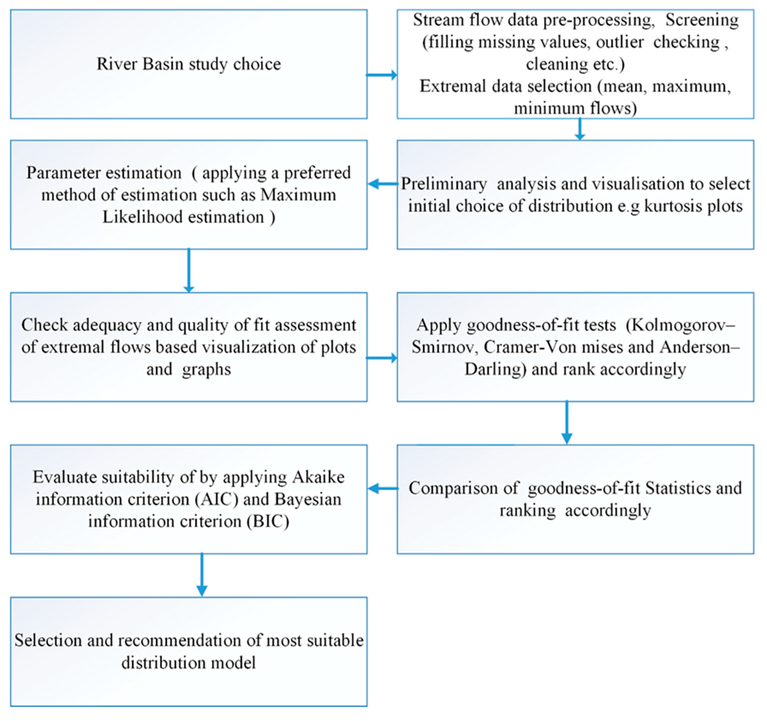
The study assesses the probability distribution for FFA; therefore, data processing and visualisation for application is a prerequisite. Firstly, classical descriptive statistics of the extremal data were processed (Table 2), and a skewness-kurtosis plot for the empirical distribution [59] showing values for common distributions was made to assist in the initial visualisation and choice of distributions to fit to the data. Thereafter, PDFs for FFA were prepared; secondly, the determination of the parameter of distributions was carried out using the MLE. Thirdly, goodness-of-fit (GoF) statistics were computed. The quality of fit was assessed using empirical and theoretical distributions, the cumulative density function, P–P and Q–Q plots, and classical goodness-of-fit statistics (Kolmogorov–Smirnov, Cramer–von Mises, and Anderson–Darling statistics [56,60]. Model estimation and selection of the best-fit distribution for the site was accomplished using information criteria-based model selection—Akaike Information Criterion (AIC) [61] and Bayesian Information Criterion (BIC) [62]—where both model estimation and selection could be simultaneously accomplished. The whole procedure and framework used in this study is as shown in Figure 2.
The method used for river discharge analysis was RStudio (2014 version), which is an integrated development environment [63] for the R programming language [64] (1996). The freely available hydroTSM [65] package in R was applied to extract and visualise the extreme data values (maximum, minimum, and mean monthly discharges) from river daily discharges. This package has robust capability functions in the management, analysis, and visualisation of the time series of hydrological flows [66]. Flood flow extreme value analysis was done by fitting a parametric distribution to the extremal data using fitdistrplus [67], which is also a free package. The package uses the maximum likelihood estimation method but also provides moment matching [8], quantile matching (QME), and maximum goodness-of fit estimation (MGE) methods. The bootstrap method [68] was used to calculate confidence intervals on quantiles of the fitted distribution from the marginal distribution of the nonparametric bootstrapped values to help understand the potential structural correlation between parameters and characterise the uncertainty in the distribution parameters [51]. The whole bootstrap sample was used to improve the estimates’ reliability [69], and also because of their importance in risk assessment.
4. Results
4.1. Preliminary Assessment and Visualisation
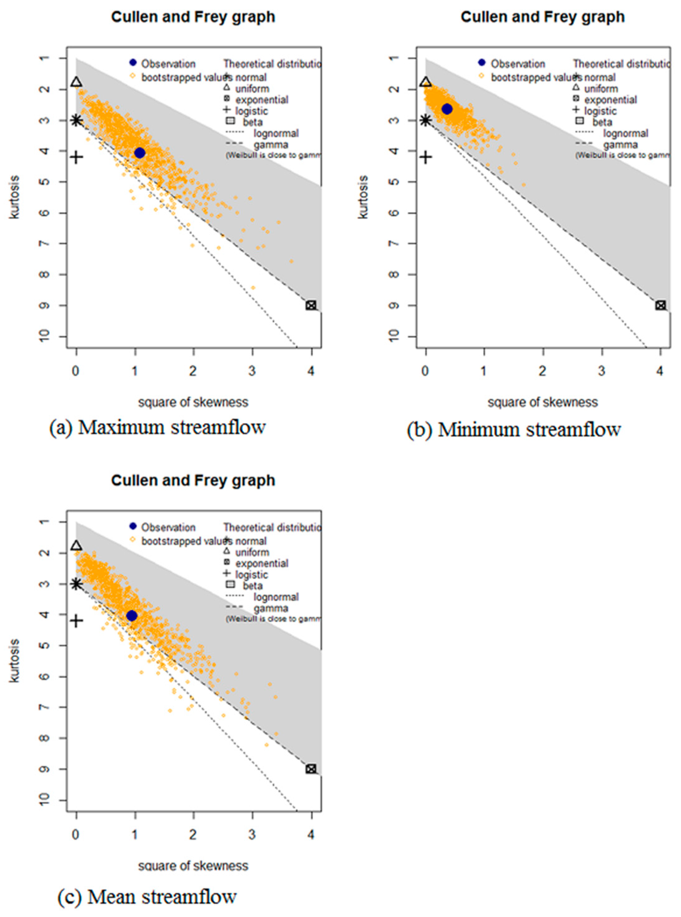
Figure 3 shows an initial skewness-kurtosis graph of the unbiased distribution [59] of the extremal data to assist in the visualisation and choice of distribution models to fit to the data. In this research, four out of the six selected models for assessment are displayed. Uniform, exponential, and logistic models have one possible value of distribution for the skewness and the kurtosis, while the possible lognormal, gamma, and Weibull areas are represented by lines, while the possible Beta areas are represented by larger areas. The kurtosis and squared skewness of extremal datasets are plotted as a blue point representing “observation” in the Cullen and Frey graph. A zero skewness shows a presence of symmetry exhibited by the empirical distribution, whereas the weight of tails as compared to the normal distribution is quantified by the kurtosis. A kurtosis value of three indicates normal distribution [59]. From Figure 3, normal, lognormal, gamma, and Weibull, being common right skewed distributions, are indicated as possible model distribution candidates because of the positive skewness and a kurtosis value that is close to three. However, the skewness and kurtosis exhibited high variations for all the distributions, and therefore, this inference can only be taken as indicative.
4.2. Goodness of Fit Using Assessment-Based Graphs
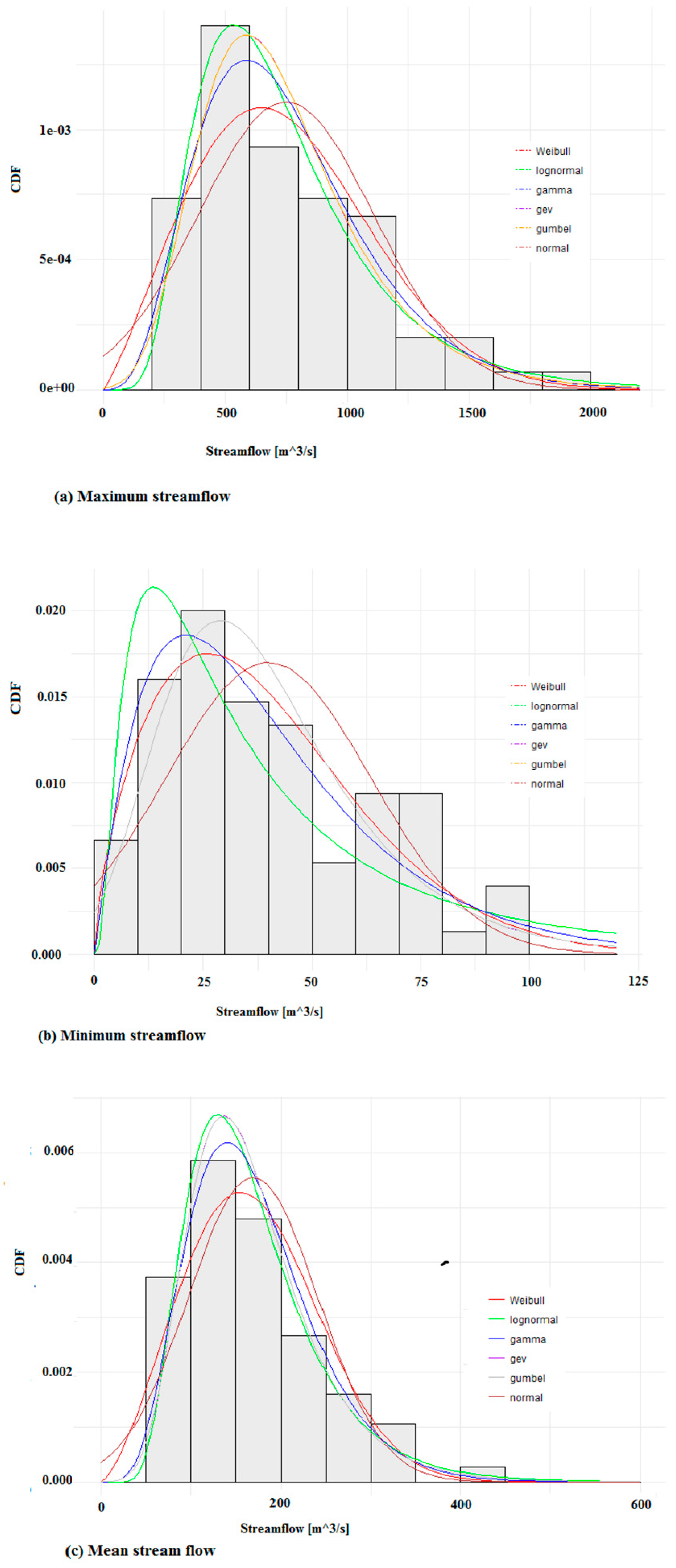
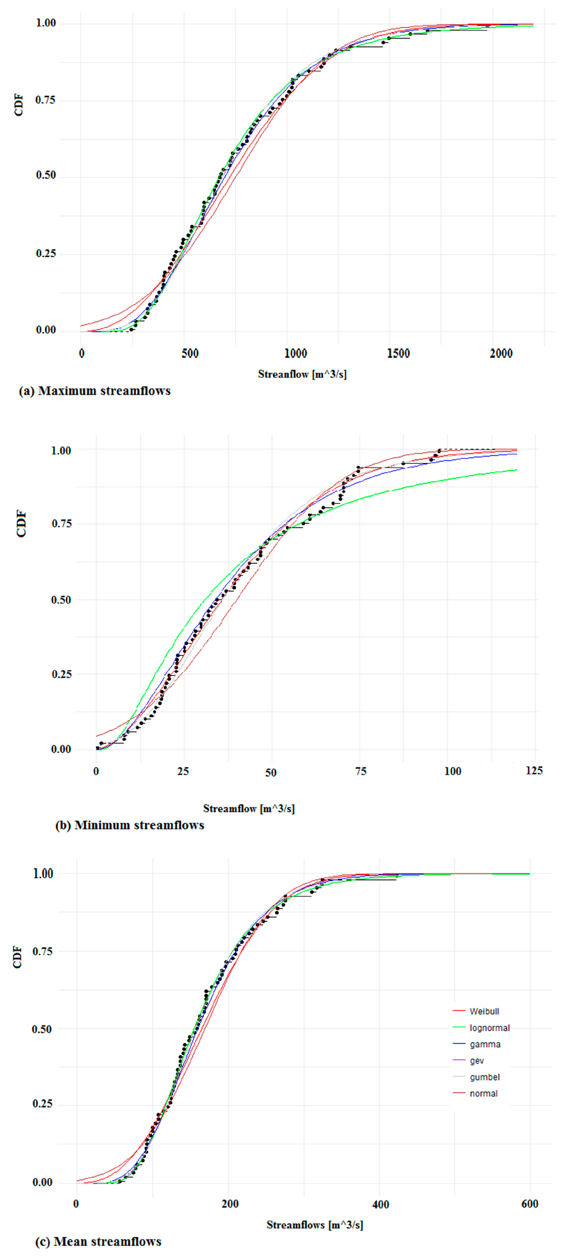
The goodness-of-fit of fitted distributions can be explored using various graphical functions. Figure 4 gives the output for the fitted six distributions to the extremal streamflow datasets using the MLE method. The histogram of the empirical distribution (data) calculated in accordance with Blom [70] superimposed with the PDF of the theoretical fitted distributions is shown in Figure 4. It illustrates the results of fitting of the six selected distribution functions to the streamflow datasets. Information on the normality or non-normality of a data is crucial in data analytics because it plays a big role in determining which algorithms may be applied and the way that the dataset should be treated. From Figure 4, the plots of the Weibull, lognormal, and gamma models seem to fit the maximum flow dataset series and thus may be the preferred models for this dataset. For low flows, the lognormal and gamma models’ loglikelihood values are heavily skewed to the left, but the Weibull and Gumbel models seem to be best suited for this dataset series. Thus, the lognormal, Weibull and gamma models are the best possible choices for mean streamflows at this site.
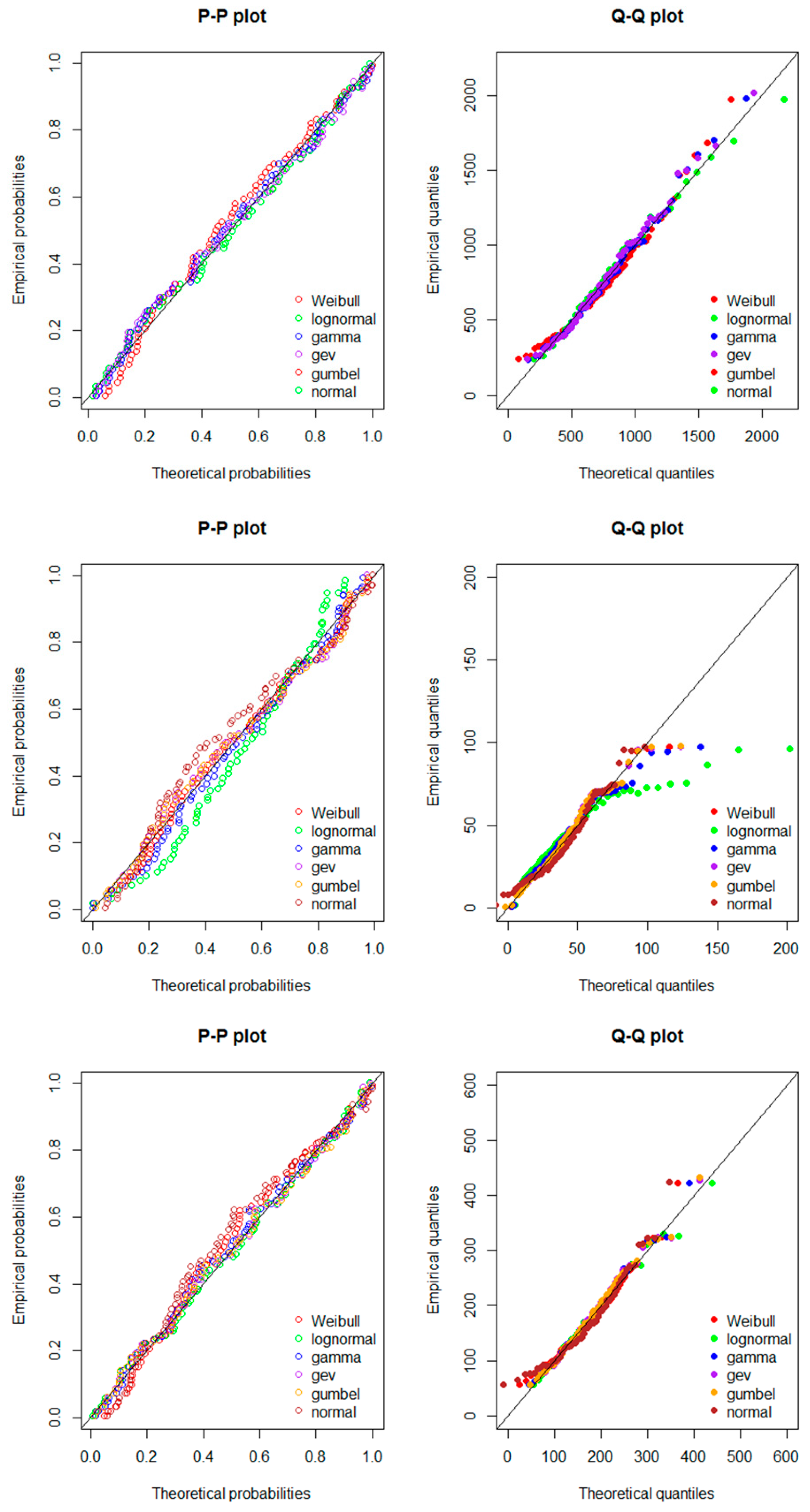
Quantile–quantile (Q–Q) plots were constructed for the graphical assessment and visualisation of the goodness of fit of the selected model distributions and to test whether or not the dataset series were derived from the six selected theoretical distributions. A probability–probability (P–P) plot is a simple graphical procedure that is used to assess the quality of the forecast prediction and assess the forecast uncertainty [71]. It plots the probability values of observed streamflow in the 0 to 1.0 range within the streamflow ensemble against a uniform distribution. If the dataset series were exactly normally distributed, then the P–P plot would be 1:1. This condition is also true for the Q–Q plot. Figure 5 shows the P–P and Q–Q plots drawn for the data series related to the maximum, minimum, and mean flows for the six selected theoretical distributions. From Figure 5, it can be seen that the P–P plots for the extremal data series are almost normally distributed. The Q–Q probability plots in Figure 5 indicate very small gaps between the fitted or theoretical line and the simulated values for all the distribution models at low and medium theoretical quantile ranges, but big gaps at high theoretical quantiles, particularly for the minimum and mean flows. Therefore, the observed data series were taken to be the true distribution, and the quantiles estimated from the observed data were also assumed to be the true quantiles of the theoretical distribution. All the selected distribution models provided a reasonable fit.
The MLE method optimises the scale and shape parameters during the computation process and provides the parameter estimates of the fitted distribution. The standard errors were calculated from the estimate of the Hessian matrix at the maximum likelihood simulation solution and the correlation matrix between the parameter estimates. The standard error (std error) indicates the reliability of the mean in a sample dataset, and that the sample mean is a more accurate representative of the actual dataset. A relatively small std error gives an indication that the mean of the sample dataset is relatively close to the true mean of the whole dataset. The probability plots simulation that is associated with the parameter estimates is shown in Table 3, and the fitted empirical and theoretical CDFs are presented in Figure 6. Inspecting the visual agreement between the simulated and fitted empirical data, it can be seen that the simulated and the observed data for all the extremal data series are very close to the y = x line, as shown in Fig. 6 and indicated by the correlation matrix in Table 3. However, large standard errors for the shape and scale parameters were returned by the Weibull, GEV, Gumbel, and normal distribution models for maximum flows. Also, the gamma (Pearson type 3), lognormal, and Weibull distributions showed large differences in errors between the shape and scale parameter estimations, which was again true for the mean flows.
4.3. GoF Test-Based Analysis
The present study considers three three-parameter distributions (gamma, GEV, and lognormal) and three two-parameter distributions (Weibull, normal, and Gumbel) in the statistical analysis. The Kolmogorov–Smirnov test, and Cramer–von Mises test were used to examine the six probability distributions at a 95% significance level (α = 0.05), as shown in Table 4. GoF test statistics were computed using Equations (3) and (4) for the extremal streamflow data that are given in Table 4. As shown in Table 3, all the classical goodness-of-fit test statistics for the Kolmogorov–Smirnov, Cramer–von Mises, and Anderson–Darling tests were acceptable at this stage for the estimation of extremal streamflow based on the test hypothesis at a 95% significance level. The computed values of test statistics are lower than the theoretical values for the six probability distributions at the chosen significance level. Each distribution was assigned a rank between one and six, with one indicating the best-fitting distribution, and six indicating the worst-fitting distribution. The goodness-of-fit tests indicated the lognormal model as the best quality of fit for the maximum streamflow dataset for Tana River at the Garissa site, followed by the gamma and GEV distribution models in the ranking order based upon the goodness-of-fit results at the site. The Weibull and normal distribution models had the least quality of performance for the maximum streamflow at this site. As for the minimum streamflow dataset, Weibull, GEV, and Gumbel showed the best goodness-of-fit statistics for all the test statistics, although GEV ranked third alongside the Anderson–Darling statistics. All three tests placed the lognormal, GEV, and Gumbel distribution models as the first, second, and third best-fit models, respectively, for the mean streamflow dataset.
4.4. Best-Fit Distribution Model
The model selection AIC uses the same response variables for all the candidate distributions while retaining all the components of each likelihood for comparing the different probability distributions and does not mingle null hypothesis testing with information criterion models. The best model is selected on the basis of the minimum AIC value calculated. The BIC, similar to the AIC, is a criterion for model selection based on the likelihood function. Lower BIC values imply both fewer explanatory variables and a better fit. The best-fit distribution is the one that best meets the criterion of the goodness-of-fit statistics and information criteria-based model selection for the extremal datasets. The results of the best-fit distribution model based on AIC and BIC within the extremal type of distribution for the Garissa site is given in Table 5.
The gamma (Pearson type 3) and lognormal distribution models were selected as the best-fitting functions for the maximum streamflows at Garissa site in the Tana River Basin due to having the lowest AIC and BIC values, as shown in Table 5. The Weibull, GEV, and Gumbel functions were the best-fit functions for the Tana River’s annual minimum flows at the site, while the lognormal and GEV distribution functions were the best-fit functions for the Tana River’s mean flows, since both the AIC and BIC returned low values. For the annual mean flows of the river, the Gumbel model seemed to be the best function with AIC, but not with BIC; this could be because BIC tends to penalise free parameters more strongly than AIC.
5. Discussion
The results obtained from maximum stream flow data series analysis by MLE for the Garissa site and its vicinity indicate that, based on most credible functions of probability distribution by AIC and BIC, lognormal and gamma (Pearson type 3), which are both three-parameter distributions, are the most suited models for maximum flood prediction studies. These findings largely agree with other recommendations elsewhere in Kenya and the world. Pearson type 3 distributions have been extensively used in the study of floods in the United States and Australia [72] since their adoption and recommendation in Bulletin 17B. Recent work recommended lognormal annual maximum flood analysis in the Tel Basin of the Mahanadi River System, India using MLE [73].
Maximum flows are related to engineering flood risks, water systems infrastructure, and developing flood response strategies, whereas mean and minimum streamflow flood frequencies are important for understanding the hydrological drought, monitoring environmental flows, irrigation, and agriculture, and managing ecosystems and natural resources. Vogel and Wilson [74] found lognormal and gamma (pearson type 3) to be the best-fit probability distributions for annual mean and minimum streamflows in 1455 river basins in the United States. The minimum streamflow (low-flow) characteristics of a stream largely govern its utilisation in terms of the type and the use economics [75]. The frequency analysis of low flows is used to determine whether an irrigation scheme needs storage or not, and for planning and designing such storage if required. However, low-flow frequency analysis has not received as much attention as maximum flows in recent years [20], despite its relevance in eastern and southern African regions where both peak floods and droughts have almost equally devastating effects. The results from this research show that the Weibull, generalised extreme value, and Gumbel distribution models are the low-flow best-fit probability distribution functions for the Tana River Basin site. However, the Weibull and Gumbel distribution models have two parameters, while the generalised extreme value distribution has three parameters. It is recommended that future research considers whether a direct statistical comparison of two-parameter and three-parameter models can have different results. Agwata [76] used an L-moments statistics approach to assess probability distributions in the Upper Tana Basin, and found that Pearson type 3 is not the best-fit model in the area, which is also reflected in this study. Elsewhere in the world, Eris, Aksoy [77] showed that the lognormal and Weibull distribution functions mostly conform to low flows in hydrological basins in Turkey [5]. Furthermore, using the maximum likelihood approach, Eris selected the Weibull function as the best probability distribution function suitable for the analysis of eight sites in the Niger Basin. The results of this research have shown that different distribution functions may be suitable for low, mean, and maximum flood frequency estimations at same site, and therefore, the choice of a suitable model for flood frequency analysis at a site with the same climatic, catchment, and hydrological characteristics depends on the frequency regime of the data series.
The MLE approach has been used in this at-site flood frequency distribution analysis and recommendations of distribution functions made for extremal streamflow data series. The MLE estimates are consistent, and the maximum likelihood estimators are asymptotically unbiased and efficient; thus, the MLE is generally preferred over the method-of-moments (MoM) approach [78]. Therefore, the recommended distributions for the frequency regimes at this site may be used to estimate the flood frequency distribution (return periods for various flood extremes and droughts) and indeed climate change impact studies to account for the non-stationarity in the area.
6. Conclusions
Flood frequency analysis is a common hydrological engineering practice and has been an active field for researchers. The paper reviews the current methods of identifying the probability distribution models in flood frequency analyses that can best describe the hydrological events of a river basin of interest. A case study is also presented where long-term flood discharge magnitudes and frequencies were extracted from streamflow data for the TRB to give an annual extremal time series for this hydrological frequency analysis. Six probability distribution models were assessed using the MLE approach, GoF tests-based analysis, and information criteria-based selection procedures to identify the most suitable distribution model for FFA for the TRB. The following conclusions are drawn from this case study analysis:
- a.
- Gamma (Pearson type 3) and lognormal distribution models were selected as the best-fit functions for maximum streamflows. The Weibull, GEV, and Gumbel functions were the best-fit functions for the Tana River annual minimum flows, while the lognormal and GEV distribution functions were the best-fit functions for the Tana River annual mean flows. The models may be used in forecasting hydrologic events, detecting the inherent stochastic characteristics of hydrologic variables, filling missing data of observations in proximal areas, and extending records for predictions and water engineering purposes.
- b.
- The GoF tests-based analysis and procedures are useful in the selection of suitable distribution model functions for the site
- c.
- Different distribution functions may be suitable for the minimum, mean, and maximum flood frequency estimations at the same site; therefore, the choice of a suitable model for flood frequency analysis at a site with the same climatic, catchment, and hydrological characteristics depends on the frequency regime of the data series.
The extremal streamflow quantile estimation methods currently in use have critical limitations and assumptions. Statistical techniques require flood data that is representative of the river basin within a reasonable period of observation, and these records need to be adjusted to reflect the changes in the characteristics of the watershed and climate variability. Also, there is a need to expand the analysis from annual to daily and seasonal daily streamflow timeseries to check whether the best-fit marginal distribution of the daily streamflow matches that of the annual extreme [79] and understand the clustering effects of short-term and long-term behavior [80,81].
Furthermore, flood data are stochastic in nature, and often assumed to be spatially and temporally independent. Practically, true probability distribution of the data at a given site or region remains uncertain. However, to date, distributions are often used to characterise the relationship between flood magnitudes, and their frequencies are evaluated to assess their performance and selected by using statistical tests. The choice of a distribution model may further be subjected to other means of selection criteria such as theoretical assessment to verify their appropriateness [82]. An upcoming paper will assess how the selected most suitable extreme distribution models affect the flood inundation at this site, including global sensitivity analysis on the input and output parameters of the flood inundation model [83]. These distribution models may be used to estimate the return periods for various flood and drought extremes at the Garissa site and its vicinity in the TRB. The continuous appraisal of streamflow using appropriate and efficient distribution models in environmental monitoring, water resources planning, sustainable agriculture, ecosystem management, and sustainable water systems infrastructure is recommended due to climate change and variability [84]. Readers are also referred to [85] for more information on the evolution of stochastic modelling for engineering applications.
Author Contributions
The conceptualisation of this research article, methodology design, analysis, and original draft were by P.K.L. Review and editing were done by L.K. and R.K.
Acknowledgments
This study did not receive any specific grant from funding agencies in the public, commercial, or not-for-profit sectors. The University of New England provided postgraduate research support to the first author. We also thank the journal’s anonymous reviewers for their constructive comments, whose help in improving the scientific quality of this manuscript is highly appreciated.
Conflicts of Interest
The authors declare that they have no conflict of interest
References
- Myronidis, D.; Stathis, D.; Sapountzis, M. Post-Evaluation of Flood Hazards Induced by Former Artificial Interventions along a Coastal Mediterranean Settlement. J. Hydrol. Eng. 2016, 21, 05016022. [Google Scholar] [CrossRef]
- Smith, J.A.; Baeck, M.L.; Villarini, G.; Wright, D.B.; Krajewski, W. Extreme flood response: The June 2008 flooding in Iowa. J. Hydrometeorol. 2013, 14, 1810–1825. [Google Scholar] [CrossRef]
- Tegos, A.; Schlüter, W.; Gibbons, N.; Katselis, Y.; Efstratiadis, A. Assessment of Environmental Flows from Complexity to Parsimony—Lessons from Lesotho. Water 2018, 10, 1293. [Google Scholar] [CrossRef]
- Srikanthan, R.; Amirthanathan, G.; Kuczera, G. Real-time flood forecasting using ensemble kalman filter. In MODSIM 2007 International Congress on Modelling and Simulation; Modelling and Simulation Society of Australia and New Zealand: Christchurch, New Zealand, 2007; pp. 1789–1795. [Google Scholar]
- Bolaji, G.; Agbede, O.; Adewumi, J.; Akinyemi, J. Selection of flood frequency model in niger basin using maximum likelihood method. In Water and Urban Development Paradigms: Towards an Integration of Engineering, Design and Management Approaches; Taylor & Francis: Abingdon, UK, 2008; p. 337. [Google Scholar]
- Cunnane, C. Statistical distributions for flood frequency analysis. In Operational Hydrology Report (WMO); WMO: Geneva, Switzerland, 1989. [Google Scholar]
- Myronidis, D.; Ioannou, K. Forecasting the urban expansion effects on the design storm hydrograph and sediment yield using artificial neural networks. Water 2019, 11, 31. [Google Scholar] [CrossRef]
- Flynn, K.M.; Kirby, W.H.; Hummel, P.R. User’s Manual for Program Peakfq, Annual Flood-Frequency Analysis Using Bulletin 17b Guidelines; U.S. Geological Survey: Reston, VA, USA, 2006; pp. 2328–7055.
- Hill, P.; Graszkiewicz, Z.; Sih, K.; Nathan, R.; Loveridge, M.; Rahman, A. Outcomes from a pilot study on modelling losses for design flood estimation. In Proceedings of the Hydrology and Water Resources Symposium 2012, Sydney, Australia, 19–22 November 2012; p. 1449. [Google Scholar]
- Loveridge, M.; Rahman, A. Probabilistic losses for design flood estimation: A case study in new south wales. In Proceedings of the Hydrology and Water Resources Symposium 2012, Sydney, Australia, 19–22 Noveber 2012; p. 9. [Google Scholar]
- Helsel, D.R.; Hirsch, R.M. Statistical Methods in Water Resources; US Geological Survey: Reston, VA, USA, 2002; Volume 323. [Google Scholar]
- Ndetei, C.; Opere, A.; Mutua, F. Flood frequency analysis in lake victoria basin based on tail behaviour of distributions. J. Kenya Meteorol. Soc. 2007, 1, 44–54. [Google Scholar]
- Khosravi, G.; Majidi, A.; Nohegar, A. Determination of suitable probability distribution for annual mean and peak discharges estimation (case study: Minab river-barantin gage, iran). Int. J. Probab. Stat. 2012, 1, 160–163. [Google Scholar] [CrossRef]
- Bobee, B.; Cavadias, G.; Ashkar, F.; Bernier, J.; Rasmussen, P. Towards a systematic approach to comparing distributions used in flood frequency analysis. J. Hydrol. 1993, 142, 121–136. [Google Scholar] [CrossRef]
- Serinaldi, F.; Kilsby, C.G.; Lombardo, F. Untenable nonstationarity: An assessment of the fitness for purpose of trend tests in hydrology. Adv. Water Resour. 2018, 111, 132–155. [Google Scholar] [CrossRef]
- Thomas, W.O., Jr. A uniform technique for flood frequency analysis. J. Water Resour. Plan. Manag. 1985, 111, 321–337. [Google Scholar] [CrossRef]
- Stedinger, J.R.; Griffis, V.W. Flood Frequency Analysis in the United States: Time to Update; American Society of Civil Engineers: Reston, VA, USA, 2008. [Google Scholar]
- Koskinas, A.; Tegos, A.; Tsira, P.; Dimitriadis, P.; Iliopoulou, T.; Papanicolaou, P.; Koutsoyiannis, D.; Williamson, T. Insights into the oroville dam 2017 spillway incident. Geosciences 2019, 9, 37. [Google Scholar]
- Olofintoye, O.; Sule, B.; Salami, A. Best–fit probability distribution model for peak daily rainfall of selected cities in nigeria. N. Y. Sci. J. 2009, 2, 1–12. [Google Scholar]
- Engeland, K.; Hisdal, H.; Frigessi, A. Practical extreme value modelling of hydrological floods and droughts: A case study. Extremes 2004, 7, 5–30. [Google Scholar] [CrossRef]
- Potter, K.W.; Lettenmaier, D.P. A comparison of regional flood frequency estimation methods using a resampling method. Water Resour. Res. 1990, 26, 415–424. [Google Scholar] [CrossRef]
- Hosking, J.R. L-moments: Analysis and estimation of distributions using linear combinations of order statistics. J. R. Stat. Soc. Ser. B (Methodol.) 1990, 105–124. [Google Scholar] [CrossRef]
- Vogel, R.M.; McMahon, T.A.; Chiew, F.H. Floodflow frequency model selection in australia. J. Hydrol. 1993, 146, 421–449. [Google Scholar] [CrossRef]
- Hoskins, J.; Wallis, J. Regional Frequency Analysis: An Approach Based on L-Moments; Cambridge University: Cambridge, UK, 1997. [Google Scholar]
- Kysely, J.; Picek, J. Regional growth curves and improved design value estimates of extreme precipitation events in the czech republic. Clim. Res. 2007, 33, 243–255. [Google Scholar] [CrossRef]
- Elamir, E.A.; Seheult, A.H. Trimmed l-moments. Comput. Stat. Data Anal. 2003, 43, 299–314. [Google Scholar] [CrossRef]
- Wang, Q.J. Lh moments for statistical analysis of extreme events. Water Resour. Res. 1997, 33, 2841–2848. [Google Scholar] [CrossRef]
- Nouri Gheidari, M.H. Comparisons of the l-and lh-moments in the selection of the best distribution for regional flood frequency analysis in lake urmia basin. Civ. Eng. Environ. Syst. 2013, 30, 72–84. [Google Scholar] [CrossRef]
- Cohn, T.; Lane, W.; Baier, W. An algorithm for computing moments-based flood quantile estimates when historical flood information is available. Water Resour. Res. 1997, 33, 2089–2096. [Google Scholar] [CrossRef]
- Griffis, V.; Stedinger, J.; Cohn, T. Log pearson type 3 quantile estimators with regional skew information and low outlier adjustments. Water Resour. Res. 2004, 40. [Google Scholar] [CrossRef]
- Greenwood, J.A.; Landwehr, J.M.; Matalas, N.C.; Wallis, J.R. Probability weighted moments: Definition and relation to parameters of several distributions expressable in inverse form. Water Resour. Res. 1979, 15, 1049–1054. [Google Scholar] [CrossRef]
- Kuczera, G. Comprehensive at-site flood frequency analysis using monte carlo bayesian inference. Water Resour. Res. 1999, 35, 1551–1557. [Google Scholar] [CrossRef]
- Ribatet, M.; Sauquet, E.; Grésillon, J.-M.; Ouarda, T.B.M.J. A regional bayesian pot model for flood frequency analysis. Stoch. Environ. Res. Risk Assess. 2007, 21, 327–339. [Google Scholar] [CrossRef]
- Ouarda, T.; El-Adlouni, S. Bayesian nonstationary frequency analysis of hydrological variables 1. J. Am. Water Resour. Assoc. 2011, 47, 496–505. [Google Scholar] [CrossRef]
- Wang, X.; Zhou, J.; Zhang, L. The probability density evolution method for flood frequency analysis: A case study of the nen river in china. Water 2015, 7, 5134–5151. [Google Scholar] [CrossRef]
- Strupczewski, W.; Singh, V.; Feluch, W. Non-stationary approach to at-site flood frequency modelling i. Maximum likelihood estimation. J. Hydrol. 2001, 248, 123–142. [Google Scholar] [CrossRef]
- Jin, M.; Stedinger, J.R. Flood frequency analysis with regional and historical information. Water Resour. Res. 1989, 25, 925–936. [Google Scholar] [CrossRef]
- Martins, E.S.; Stedinger, J.R. Generalized maximum-likelihood generalized extreme-value quantile estimators for hydrologic data. Water Resour. Res. 2000, 36, 737–744. [Google Scholar] [CrossRef]
- Hosking, J.R. Moments or l moments? An example comparing two measures of distributional shape. Am. Stat. 1992, 46, 186–189. [Google Scholar] [CrossRef]
- Madsen, H.; Pearson, C.P.; Rosbjerg, D. Comparison of annual maximum series and partial duration series methods for modeling extreme hydrologic events: 2. Regional modeling. Water Resour. Res. 1997, 33, 759–769. [Google Scholar] [CrossRef]
- Laio, F.; Di Baldassarre, G.; Montanari, A. Model selection techniques for the frequency analysis of hydrological extremes. Water Resour. Res. 2009, 45. [Google Scholar] [CrossRef]
- Haddad, K.; Rahman, A. Selection of the best fit flood frequency distribution and parameter estimation procedure: A case study for tasmania in australia. Stoch. Environ. Res. Risk Assess. 2011, 25, 415–428. [Google Scholar] [CrossRef]
- Griffis, V.; Stedinger, J. Log-pearson type 3 distribution and its application in flood frequency analysis. I: Distribution characteristics. J. Hydrol. Eng. 2007, 12, 482–491. [Google Scholar] [CrossRef]
- Rahman, A.S.; Rahman, A.; Zaman, M.A.; Haddad, K.; Ahsan, A.; Imteaz, M. A study on selection of probability distributions for at-site flood frequency analysis in australia. Natural Hazards 2013, 69, 1803–1813. [Google Scholar] [CrossRef]
- Vogel, R.M.; Thomas, W.O., Jr.; McMahon, T.A. Flood-flow frequency model selection in southwestern united states. J. Water Resour. Plan. Manag. 1993, 119, 353–366. [Google Scholar] [CrossRef]
- Langat, P.K.; Kumar, L.; Koech, R. Understanding water and land use within tana and athi river basins in kenya: Opportunities for improvement. Sustain. Water Resour. Manag. 2018, 1–11. [Google Scholar] [CrossRef]
- van Beukering, P.; de Moel, H.; Botzen, W.; Eiselin, M.; Kamau, P.; Lange, K.; van Maanen, E.; Mogol, S.; Mulwa, R.; Otieno, P. The economics of ecosystem services of the tana river basin-assessment of the impact of large infrastructural interventions. R-Report 2015, 15, 3. [Google Scholar]
- Saji, N.; Goswami, B.; Vinayachandran, P.; Yamagata, T. A dipole mode in the tropical indian ocean. Nature 1999, 401, 360. [Google Scholar] [CrossRef]
- Birkett, C.; Murtugudde, R.; Allan, T. Indian ocean climate event brings floods to east africa’s lakes and the sudd marsh. Geophys. Res. Lett. 1999, 26, 1031–1034. [Google Scholar] [CrossRef]
- Koei, N. The Project on the Development of the National Water Master Plan 2030; Final Report; Volume v Sectoral Report (e)—Agriculture and Irrigation; the Republic of Kenya; Water Resources Management Authority: Nairobi, Kenya, 2013.
- Langat, P.K.; Kumar, L.; Koech, R. Temporal variability and trends of rainfall and streamflow in tana river basin, kenya. Sustainability 2017, 9, 1963. [Google Scholar] [CrossRef]
- Seckin, N.; Yurtal, R.; Haktanir, T.; Dogan, A. Comparison of probability weighted moments and maximum likelihood methods used in flood frequency analysis for ceyhan river basin. Arab. J. Sci. Eng. 2010, 35, 49. [Google Scholar]
- Ojha, C.; Berndtsson, R.; Bhunya, P.A. Books published. Environ. Manag. 2009, 1, 117–131. [Google Scholar]
- Rao, A.; Hamed, K. The logistic distribution. In Flood Frequency Analysis; CRC Press: Boca Raton, FL, USA, 2000; pp. 291–321. [Google Scholar]
- Zhang, J. Powerful goodness-of-fit tests based on the likelihood ratio. J. R. Stat.Soc. Ser. B (Stat. Methodol.) 2002, 64, 281–294. [Google Scholar] [CrossRef]
- Anderson, T.W.; Darling, D.A. Asymptotic theory of certain” goodness of fit” criteria based on stochastic processes. Ann. Math. Stat. 1952, 23, 193–212. [Google Scholar] [CrossRef]
- Chakravarti, I.M.; Laha, R.G.; Roy, J. Handbook of Methods of Applied Statistics; Wiley Series in Probability and Mathematical Statistics (USA) eng; Wiley: Hoboken, NJ, USA, 1967. [Google Scholar]
- Stephens, M.A. Tests based on edf statistics. In Goodness-of-Fit Techniques; d’agostino, R.B., Stephens, M.A., Eds.; Marcel Dekker: New York, NY, USA, 1986; pp. 1–15. [Google Scholar]
- Cullen, A.C.; Frey, H.C.; Frey, C.H. Probabilistic Techniques in Exposure Assessment: A Handbook for Dealing with Variability and Uncertainty in Models and Inputs; Springer Science & Business Media: New York, NY, USA, 1999. [Google Scholar]
- D’Agostino, R.B.; Stephens, M.A. Goodness-fo-Fit-Techniques; Taylor & Francis: Abingdon, UK, 1986. [Google Scholar]
- Akaike, H. Information theory and an extension of the maximum likelihood principle. In Selected Papers of Hirotugu Akaike; Springer: Berlin/Heidelberg, Germany, 1998; pp. 199–213. [Google Scholar]
- Raftery, A.E. Bayesian model selection in social research. Sociol. Methodol. 1995, 25, 111–163. [Google Scholar] [CrossRef]
- Dewan, A.; Corner, R.; Saleem, A.; Rahman, M.M.; Haider, M.R.; Rahman, M.M.; Sarker, M.H. Assessing channel changes of the ganges-padma river system in bangladesh using landsat and hydrological data. Geomorphology 2017, 276, 257–279. [Google Scholar] [CrossRef]
- Ihaka, R.; Gentleman, R. R: A language for data analysis and graphics. J. Comput. Graph. Stat. 1996, 5, 299–314. [Google Scholar]
- Zambrano-Bigiarini, M. Package ‘hydroTSM: Time Series Management, Analyis and Interpolation for Hydrological Modelling. 2017. Available online: https://cran.r-project.org/package=hydroTSM (accessed on 25 October 2017).
- Cisty, M.; Celar, L. Using r in water resources education. Int. J. Innov. Educ. Res. 2015, 3, 97–117. [Google Scholar]
- Delignette-Muller, M.L.; Dutang, C.; Pouillot, R.; Denis, J.-B.; Siberchicot, A.; Siberchicot, M.A. Package ‘fitdistrplus’. R Foundation for Statistical Computing, Vienna, Austria. 2017. Available online: http://www. R-project. org (accessed on 25 October 2017).
- Babu, G.J.; Rao, C. Goodness-of-fit tests when parameters are estimated. Sankhya 2004, 66, 63–74. [Google Scholar]
- Volpi, E.; Fiori, A.; Grimaldi, S.; Lombardo, F.; Koutsoyiannis, D. Save hydrological observations! Return period estimation without data decimation. J. Hydrol. 2019, 571, 782–792. [Google Scholar] [CrossRef]
- Blom, G. Statistical Estimates and Transformed Beta Variables; Wiley: New York, NY, USA, 1958. [Google Scholar]
- Thyer, M.; Renard, B.; Kavetski, D.; Kuczera, G.; Franks, S.W.; Srikanthan, S. Critical evaluation of parameter consistency and predictive uncertainty in hydrological modeling: A case study using bayesian total error analysis. Water Resour. Res. 2009, 45. [Google Scholar] [CrossRef]
- Beard, L.R. Book review: The gamma family and derived distributions applied in hydrology. By bernard bobee and fahim ashkar, water resources publications, littleton, co 80161-2841, USA, 1991, 203 pp., soft cover, $38.00, isbn 0-918334-68-3. J. Hydrol. 1992, 132, 383. [Google Scholar] [CrossRef]
- Guru, N.; Jha, R. Flood frequency analysis of tel basin of mahanadi river system, india using annual maximum and pot flood data. Aquat. Procedia 2015, 4, 427–434. [Google Scholar] [CrossRef]
- Vogel, R.M.; Wilson, I. Probability distribution of annual maximum, mean, and minimum streamflows in the united states. J. Hydrol. Eng. 1996, 1, 69–76. [Google Scholar] [CrossRef]
- Survey, G.; Speer, P.R.; Golden, H.G. Low-Flow Characteristics of Streams in the Mississippi Embayment in Mississippi and Alabama; US Government Printing Office: Washington, DC, USA, 1964.
- Agwata, J.F. Water resources utilization, conflicts and interventions in the tana basin of Kenya. FWU Water Resour. Publ. 2005, 3, 13–23. [Google Scholar]
- Eris, E.; Aksoy, H.; Onoz, B.; Cetin, M.; Yuce, M.I.; Selek, B.; Aksu, H.; Burgan, H.I.; Esit, M.; Yildirim, I. Frequency analysis of low flows in intermittent and non-intermittent rivers from hydrological basins in turkey. Water Sci. Technol. Water Supp. 2019, 19, 30–39. [Google Scholar] [CrossRef]
- Laio, F. Cramer–von mises and anderson-darling goodness of fit tests for extreme value distributions with unknown parameters. Water Resour. Res. 2004, 40. [Google Scholar] [CrossRef]
- Blum, A.G.; Archfield, S.A.; Vogel, R.M. On the probability distribution of daily streamflow in the united states. Hydrol. Earth Syst. Sci. 2017, 21, 3093–3103. [Google Scholar] [CrossRef]
- Dimitriadis, P.; Koutsoyiannis, D. Stochastic synthesis approximating any process dependence and distribution. Stoch. Environ. Res. Risk Assess. 2018, 32, 1493–1515. [Google Scholar] [CrossRef]
- Dimitriadis, P.; Koutsoyiannis, D. Climacogram versus autocovariance and power spectrum in stochastic modelling for markovian and hurst–kolmogorov processes. Stoch. Environ. Res. Risk Assess. 2015, 29, 1649–1669. [Google Scholar] [CrossRef]
- Koutsoyiannis, D. Statistics of extremes and estimation of extreme rainfall: I. Theoretical investigation/statistiques de valeurs extrêmes et estimation de précipitations extrêmes: I. Recherche théorique. Hydrol. Sci. J. 2004, 49. [Google Scholar] [CrossRef]
- Dimitriadis, P.; Tegos, A.; Oikonomou, A.; Pagana, V.; Koukouvinos, A.; Mamassis, N.; Koutsoyiannis, D.; Efstratiadis, A. Comparative evaluation of 1d and quasi-2d hydraulic models based on benchmark and real-world applications for uncertainty assessment in flood mapping. J. Hydrol. 2016, 534, 478–492. [Google Scholar] [CrossRef]
- Ngongondo, C.; Li, L.; Gong, L.; Xu, C.-Y.; Alemaw, B.F. Flood frequency under changing climate in the upper kafue river basin, southern africa: A large scale hydrological model application. Stoch. Environ. Res. Risk Assess. 2013, 27, 1883–1898. [Google Scholar] [CrossRef]
- Koutsoyiannis, D. Generic and parsimonious stochastic modelling for hydrology and beyond. Hydrol. Sci. J. 2016, 61, 225–244. [Google Scholar] [CrossRef]
Figure 1.
Map of the study area showing the geographic features of the Tana River Basin (TRB) in Kenya, including the Tana River stream system in detail, the lower Tana floodplains and wetlands, and the Garissa hydrometric station used in the study.
Figure 1.
Map of the study area showing the geographic features of the Tana River Basin (TRB) in Kenya, including the Tana River stream system in detail, the lower Tana floodplains and wetlands, and the Garissa hydrometric station used in the study.

Figure 2.
Flowchart for data analysis, fitting test, and evaluation and selection of the appropriate distribution model.
Figure 2.
Flowchart for data analysis, fitting test, and evaluation and selection of the appropriate distribution model.

Figure 3.
Description of extreme streamflow samples from a normal distribution with uncertainty on skewness and kurtosis estimated by bootstrap. The extreme floods are (a) maximum streamflow, (b) minimum streamflow and (c) mean streamflow.
Figure 3.
Description of extreme streamflow samples from a normal distribution with uncertainty on skewness and kurtosis estimated by bootstrap. The extreme floods are (a) maximum streamflow, (b) minimum streamflow and (c) mean streamflow.

Figure 4.
Fitted Cumulative distribution functions (CDF) of the six selected distribution models: (a) maximum streamflow, (b) minimum streamflow, and (c) mean streamflow.
Figure 4.
Fitted Cumulative distribution functions (CDF) of the six selected distribution models: (a) maximum streamflow, (b) minimum streamflow, and (c) mean streamflow.

Figure 5.
Probability–probability (P–P) and quantile–quantile (Q–Q) plots for the observed daily.

Figure 6.
Fitted empirical and theoretical CDFs of the Tana River extremal daily data series (a) maximum streamflow, (b) minimum streamflow and (c) mean streamflow.
Figure 6.
Fitted empirical and theoretical CDFs of the Tana River extremal daily data series (a) maximum streamflow, (b) minimum streamflow and (c) mean streamflow.


Table 1.
General description of distribution functions and their ranges used in this study. GEV: generalised extreme value.
Table 1.
General description of distribution functions and their ranges used in this study. GEV: generalised extreme value.
| Distribution Model | Probability Distribution Function (PDF) | Range |
|---|---|---|
| Gamma (Pearson type 3) | Q ≥ 0, α, β > 0 | |
| Lognormal | < Q < | |
| Weibull | ||
| GEV | Q > for | |
| Gumbel | ||
| Normal |
Γ = the gamma function, F = cumulative density function of Q.
Table 2.
Classical descriptive statistics for Tana River extremal daily discharge (1941–2016) at the Garissa river gauging station.
Table 2.
Classical descriptive statistics for Tana River extremal daily discharge (1941–2016) at the Garissa river gauging station.
| Statistic | Extreme Streamflow Datasets | ||
|---|---|---|---|
| Maximum Streamflow | Minimum Streamflow | Mean Streamflow | |
| Minimum (m3/s) | 244.89 | 0.22 | 56.73 |
| Maximum (m3/s) | 1974.02 | 97.61 | 423.04 |
| Median (m3/s) | 674.05 | 34.37 | 157.93 |
| Mean (m3/s) | 749.22 | 39.98 | 169.21 |
| Estimated standard deviation (m3/s) | 363.10 | 23.65 | 72.29 |
| Estimated skewness | 1.04 | 0.62 | 0.98 |
| Estimated kurtosis | 4.063 | 2.645 | 4.048 |
Table 3.
Distribution sample estimates, standard errors, and correlation matrix of parameter shape and scale values estimated using the maximum likelihood estimation (MLE) method.
Table 3.
Distribution sample estimates, standard errors, and correlation matrix of parameter shape and scale values estimated using the maximum likelihood estimation (MLE) method.
| Maximum Flows | Minimum Flows | Mean Flows | |||||||||||
|---|---|---|---|---|---|---|---|---|---|---|---|---|---|
| Distribution | Standard Error | Correlation Matrix | Standard Error | Correlation Matrix | Standard Error | Correlation Matrix | |||||||
| Sample estimate | Standard Error | Shape | Scale | Sample Estimate | Standard Error | Shape | Scale | Sample estimate | Standard Error | Shape | Scale | ||
| Gamma (Pearson type 3) | shape | 4.65 | 0.64 | 1.00 | 0.93 | 2.11 | 0.32 | 1.00 | 0.89 | 5.92 | 0.93 | 1.00 | 0.96 |
| scale | 0.01 | 0.00 | 0.93 | 1.00 | 0.05 | 0.01 | 0.89 | 1.00 | 0.03 | 0.01 | 0.96 | 1.00 | |
| Lognormal | shape | 6.51 | 0.48 | 1.00 | 0.00 | 3.43 | 0.11 | 0.00 | 1.00 | 5.04 | 0.05 | 1.00 | 0.00 |
| scale | 0.05 | 0.04 | 0.00 | 1.00 | 0.91 | 0.07 | 1.00 | 0.00 | 0.42 | 0.03 | 0.00 | 1.00 | |
| Weibull | shape | 2.22 | 0.19 | 1.00 | 0.33 | 1.68 | 0.16 | 1.00 | 0.30 | 2.50 | 0.05 | 1.00 | 0.00 |
| scale | 849.40 | 46.93 | 0.33 | 1.00 | 44.49 | 3.20 | 0.30 | 1.00 | 0.42 | 0.03 | 0.00 | 1.00 | |
| GEV | shape | 587.02 | 32.71 | 1.00 | 0.31 | 28.99 | 2.30 | 1.00 | 0.32 | 136.67 | 6.70 | 1.00 | 0.31 |
| scale | 269.54 | 25.18 | 0.31 | 1.00 | 18.92 | 1.73 | 0.32 | 1.00 | 55.12 | 5.08 | 0.31 | 1.00 | |
| Gumbel | shape | 587.07 | 32.72 | 1.00 | 0.31 | 28.99 | 2.30 | 1.00 | 0.32 | 136.66 | 6.70 | 1.00 | 0.31 |
| scale | 269.62 | 25.20 | 0.31 | 1.00 | 18.92 | 1.73 | 0.32 | 1.00 | 55.17 | 5.09 | 0.31 | 1.00 | |
| Normal | shape | 749.22 | 41.65 | 1.00 | 0.00 | 39.98 | 2.71 | 1.00 | 0.00 | 169.21 | 8.29 | 1.00 | 0.00 |
| scale | 360.66 | 29.45 | 0.00 | 1.00 | 23.49 | 1.92 | 0.00 | 1.00 | 71.81 | 5.86 | 0.00 | 1.00 | |
Table 4.
Fitted distributions to extremal Tana River streamflow data by maximum likelihood estimation and comparison of goodness-of-fit statistics.
Table 4.
Fitted distributions to extremal Tana River streamflow data by maximum likelihood estimation and comparison of goodness-of-fit statistics.
| Distribution | Kolmogorov–Smirnov (Critical Value at 0.05 = 0.20517) | Cramer–von Mises (Critical Value at 0.05 = 0.221) | Anderson–Darling (Critical Value at 0.05 = 2.5018) | |||
|---|---|---|---|---|---|---|
| Statistic | Rank | Statistic | Rank | Statistic | Rank | |
| Maximum Streamflow | ||||||
| Gamma (Pearson type 3) | 0.0568 | 2 | 0.0377 | 2 | 0.2771 | 2 |
| Lognormal | 0.0545 | 1 | 0.0307 | 1 | 0.2048 | 1 |
| Weibull | 0.0705 | 5 | 0.0845 | 5 | 0.6521 | 5 |
| GEV | 0.0635 | 3 | 0.0452 | 3 | 0.3294 | 3 |
| Gumbel | 0.0692 | 4 | 0.0633 | 4 | 0.4271 | 4 |
| Normal | 0.1011 | 6 | 0.2088 | 6 | 1.2463 | 6 |
| Minimum Streamflow | ||||||
| Gamma (Pearson type 3) | 0.0711 | 4 | 0.0668 | 4 | 0.6331 | 4 |
| Lognormal | 0.1296 | 6 | 0.3389 | 6 | 2.4926 | 6 |
| Weibull | 0.0549 | 1 | 0.0411 | 1 | 0.4007 | 1 |
| GEV | 0.0693 | 2 | 0.0633 | 2 | 0.4272 | 3 |
| Gumbel | 0.0693 | 2 | 0.0633 | 2 | 0.4271 | 2 |
| Normal | 0.1011 | 5 | 0.2088 | 5 | 1.2463 | 5 |
| Mean Streamflow | ||||||
| Gamma (Pearson type 3) | 0.0621 | 4 | 0.0349 | 4 | 0.2341 | 4 |
| Lognormal | 0.0410 | 1 | 0.0193 | 1 | 0.1425 | 1 |
| Weibull | 0.0956 | 5 | 0.1068 | 5 | 0.7245 | 5 |
| GEV | 0.0455 | 3 | 0.0269 | 3 | 0.1988 | 3 |
| Gumbel | 0.0453 | 2 | 0.0267 | 2 | 0.1972 | 2 |
| Normal | 0.1168 | 6 | 0.1883 | 6 | 1.1685 | 6 |
Table 5.
Goodness-of-fit information criterion. AIC: Akaike Information Criterion, BIC: Bayesian Information Criterion.
Table 5.
Goodness-of-fit information criterion. AIC: Akaike Information Criterion, BIC: Bayesian Information Criterion.
| Distribution | Maximum Streamflow | Minimum Streamflow | Mean Streamflow | |||
|---|---|---|---|---|---|---|
| AIC | BIC | AIC | BIC | AIC | BIC | |
| Gamma (Pearson type 3) | 1083.1 | 1087.7 | 687.3 | 691.9 | 844.4 | 849.0 |
| Lognormal | 1081.4 | 1086.0 | 718.0 | 722.7 | 843.2 | 847.8 |
| Weibull | 1089.5 | 1094.1 | 682.1 | 686.8 | 851.5 | 856.2 |
| GEV | 1083.7 | 1088.4 | 682.2 | 686.8 | 844.1 | 848.7 |
| Gumbel | 1083.7 | 1088.4 | 682.2 | 686.8 | 844.1 | 857.9 |
| Normal | 1100.0 | 1104.7 | 690.3 | 694.9 | 848.7 | 862.6 |
© 2019 by the authors. Licensee MDPI, Basel, Switzerland. This article is an open access article distributed under the terms and conditions of the Creative Commons Attribution (CC BY) license (http://creativecommons.org/licenses/by/4.0/).
Share and Cite
MDPI and ACS Style
Langat, P.K.; Kumar, L.; Koech, R. Identification of the Most Suitable Probability Distribution Models for Maximum, Minimum, and Mean Streamflow. Water 2019, 11, 734. https://doi.org/10.3390/w11040734
AMA Style
Langat PK, Kumar L, Koech R. Identification of the Most Suitable Probability Distribution Models for Maximum, Minimum, and Mean Streamflow. Water. 2019; 11(4):734. https://doi.org/10.3390/w11040734
Chicago/Turabian StyleLangat, Philip Kibet, Lalit Kumar, and Richard Koech. 2019. "Identification of the Most Suitable Probability Distribution Models for Maximum, Minimum, and Mean Streamflow" Water 11, no. 4: 734. https://doi.org/10.3390/w11040734
Note that from the first issue of 2016, this journal uses article numbers instead of page numbers. See further details here.