Empirical Validation of MesoHABSIM Models Developed with Different Habitat Suitability Criteria for Bullhead Cottus Gobio L. as an Indicator Species

 , , , and
Abstract
:1. Introduction
- (1)
- Which of the two methods (inductive or deductive) more accurately describes the habitat suitability of aquatic organisms?
- (2)
- Are the results of both approaches even comparable or would they lead to drastically different conclusions and therefore management actions?
2. Materials and Methods
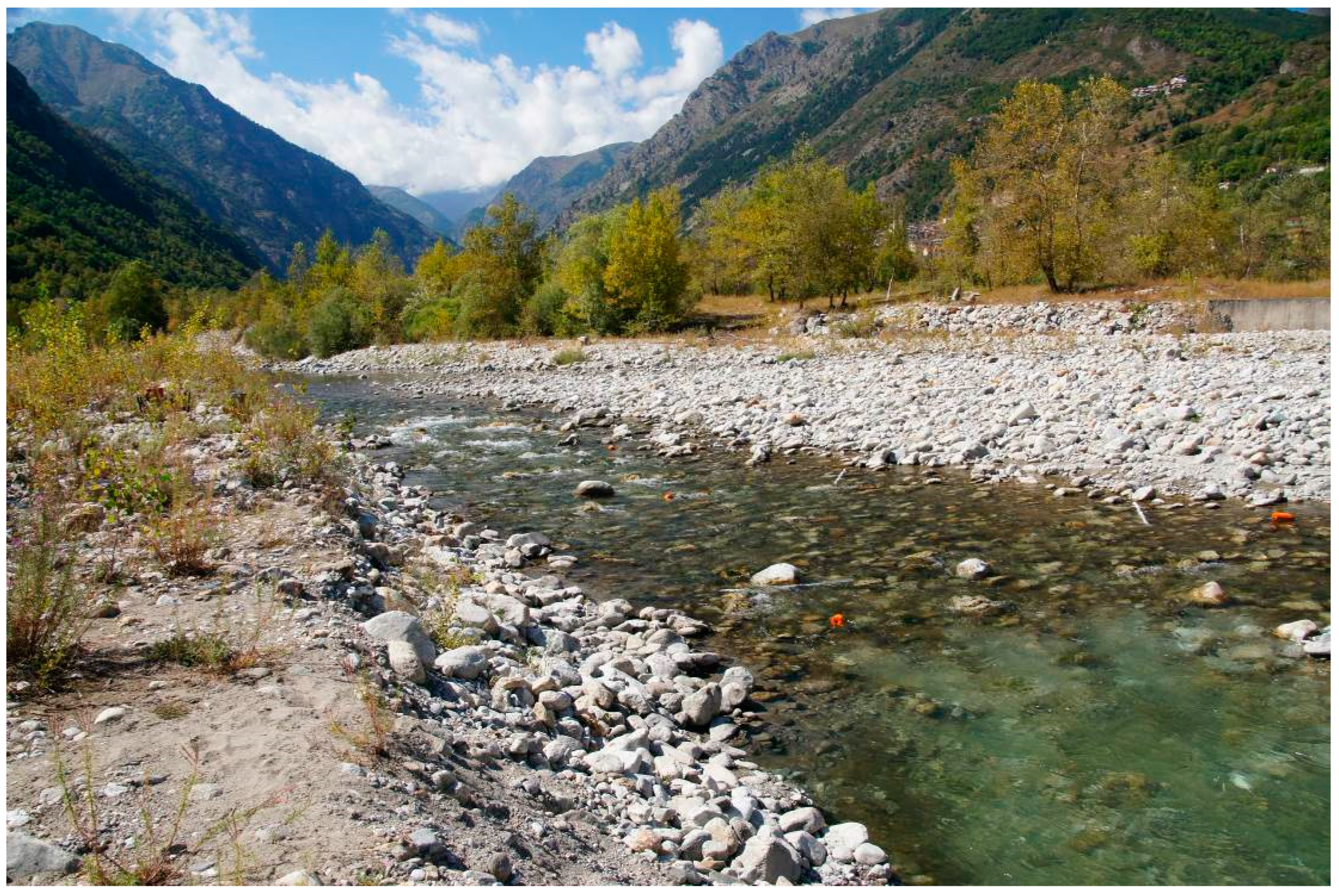
2.1. Study Area
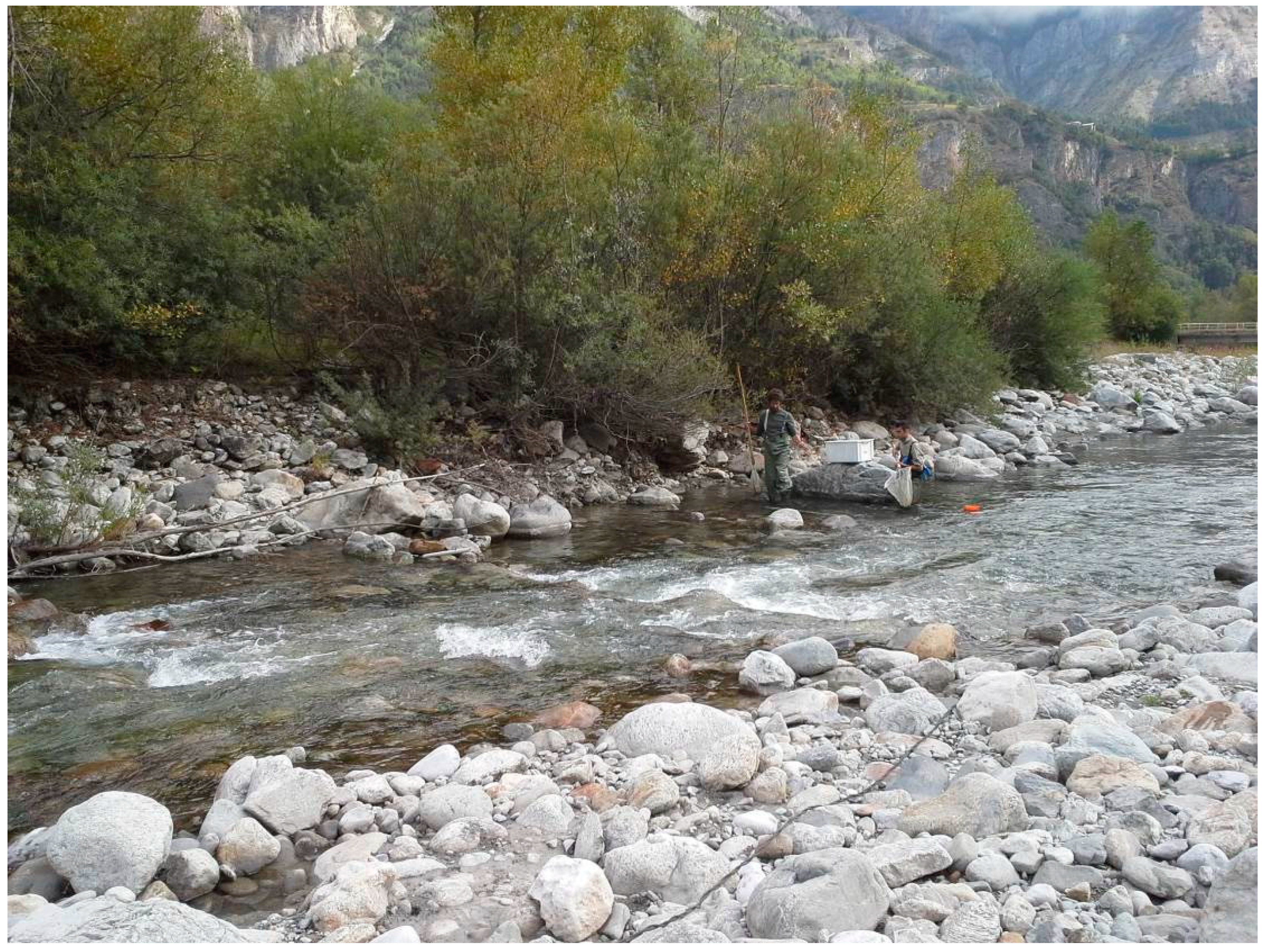
2.2. Habitat Mapping and Electrofishing
2.3. Indicator Species
2.4. Models
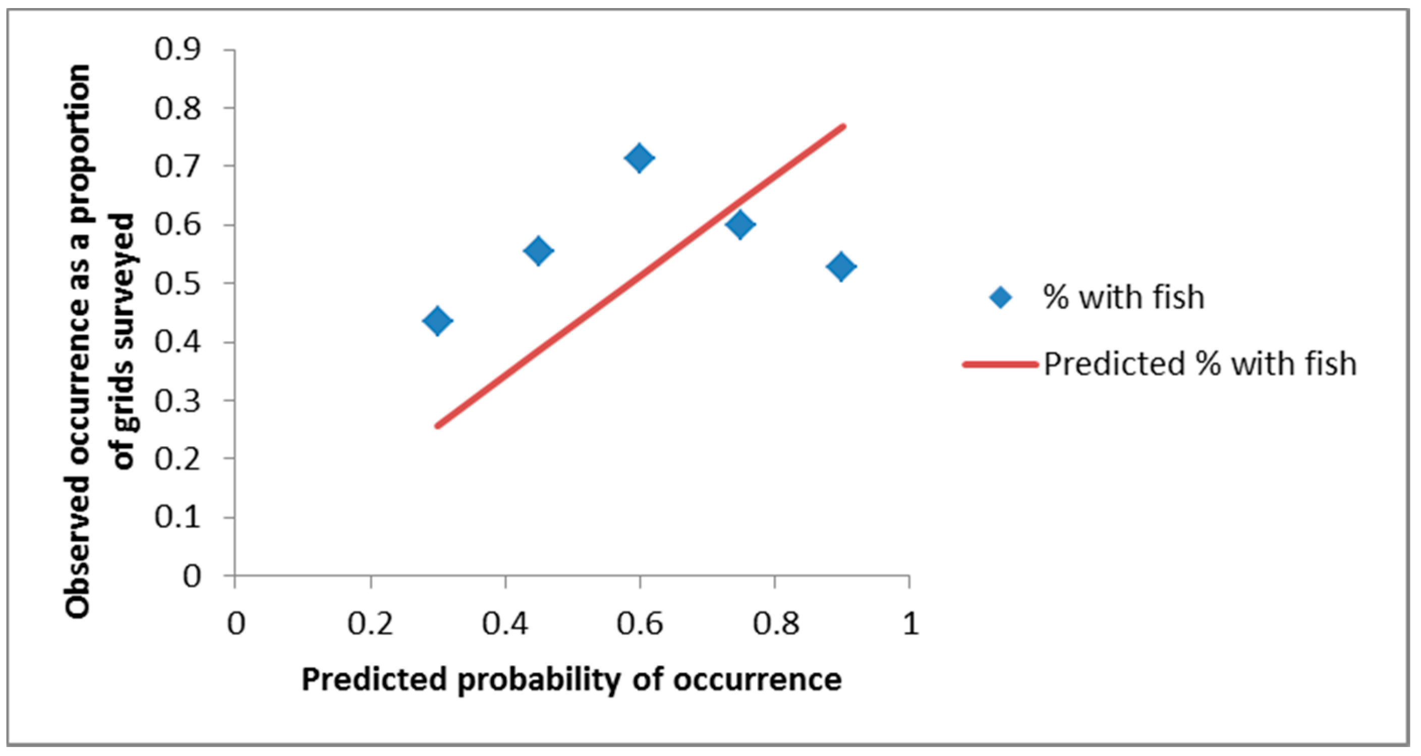
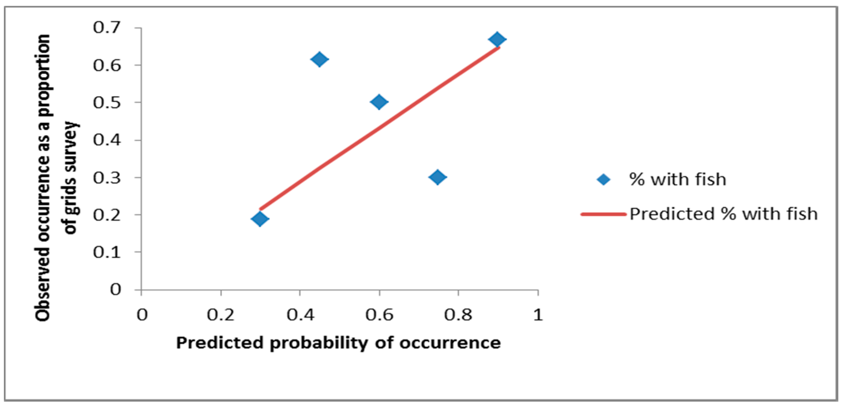
3. Results
4. Discussion
5. Conclusions
- (1)
- Inductive and deductive models do not offer statistically identical results, and the choice of model can have some influence on the results.
- (2)
- Lowering the cutoff value in a standard statistical model results in greater similarity to the CHSC model (Spearman rank correlation).
- (3)
- The statistical model underestimates suitable habitats and is more appropriate for endangered species studies according to precautionary principle.
- (4)
- Application of properly constructed MesoHABSIM literature-based models complemented by expert opinion like the CHSC model provides more generic information about habitat suitability.
- (5)
- Nevertheless, the CHSC model validated very well and beyond expectations. It could easily be better calibrated with a relatively small sample of field data.
Author Contributions
Funding
Acknowledgments
Conflicts of Interest
Appendix

| HMU No | HMU Type | GRID No | SPECIES | Sum | ||
|---|---|---|---|---|---|---|
| Brown Trout | Bullhead | Fallfish | ||||
| 11001 | RAPID | 1 | 9 | 9 | ||
| 2 | 5 | 5 | ||||
| 3 | 3 | 3 | ||||
| 4 | 1 | 1 | ||||
| 11002 | RIFFLE | 1 | 1 | 4 | 5 | |
| 2 | 0 | |||||
| 3 | 4 | 4 | ||||
| 4 | 0 | |||||
| 5 | 1 | 1 | ||||
| 11003 | SIDEARM | 1 | 0 | |||
| 2 | 0 | |||||
| 3 | 1 | 1 | ||||
| 4 | 1 | 1 | ||||
| 5 | 0 | |||||
| 11004 | RIFFLE | 1 | 1 | 3 | 4 | |
| 2 | 2 | 2 | ||||
| 3 | 0 | |||||
| 4 | 2 | 2 | ||||
| 5 | 1 | 2 | 3 | |||
| 11005 | RIFFLE | 1 | 1 | 4 | 5 | |
| 2 | 0 | |||||
| 3 | 2 | 4 | 6 | |||
| 11006 | COMPLEXHIGH | 1 | 0 | |||
| 2 | 0 | |||||
| 11007 | GLIDE | 1 | 5 | 5 | ||
| 2 | 5 | 5 | ||||
| 3 | 1 | 1 | ||||
| 4 | 2 | 2 | ||||
| 5 | 1 | 1 | ||||
| 11008 | PLUNGEPOOL | 1 | 1 | 4 | 5 | |
| 2 | 4 | 2 | 6 | |||
| 3 | 2 | 3 | 5 | |||
| 4 | 3 | 2 | 5 | |||
| 11009 | RAPID | 1 | 2 | 2 | ||
| 2 | 2 | 1 | 3 | |||
| 11010 | RIFFLE | 1 | 5 | 5 | ||
| 2 | 1 | 1 | ||||
| 3 | 1 | 1 | ||||
| 11011 | GLIDE | 1 | 1 | 1 | 2 | |
| 2 | 5 | 5 | ||||
| 3 | 2 | 2 | ||||
| 4 | 1 | 1 | ||||
| 11012 | POOL | 1 | 1 | 1 | ||
| 2 | 2 | 2 | ||||
| 3 | 0 | |||||
| 4 | 3 | 3 | ||||
| 5 | 0 | |||||
| 11013 | RUFFLE | 1 | 2 | 2 | ||
| 2 | 0 | |||||
| 3 | 1 | 1 | ||||
| 11014 | RAPID | 1 | 1 | 1 | ||
| 2 | 5 | 5 | ||||
| 21001 | BACKWATER | 1 | 0 | |||
| 2 | 0 | |||||
| 21002 | SIDEARM | 1 | 0 | |||
| 2 | 0 | |||||
| 21003 | POOL | 1 | 0 | |||
| 2 | 0 | |||||
| 21004 | RUFFLE | 1 | 1 | 1 | ||
| 2 | 2 | 2 | ||||
| 3 | 2 | 2 | ||||
| 4 | 0 | |||||
| 5 | 1 | 1 | ||||
| 21005 | RAPID | 1 | 0 | |||
| 2 | 0 | |||||
| 3 | 2 | 2 | ||||
| 4 | 2 | 2 | ||||
| 5 | 0 | |||||
| 21006 | COMPLEXHIGH | 1 | 2 | 2 | ||
| 2 | 0 | |||||
| 3 | 1 | 1 | ||||
| 21007 | SIDEARM | 1 | 1 | 1 | 2 | |
| 2 | 0 | |||||
| 21008 | RUFFLE | 1 | 1 | 1 | ||
| 2 | 2 | 2 | ||||
| 3 | 1 | 1 | ||||
| 21009 | COMPLEXHIGH | 1 | 0 | |||
| 2 | 0 | |||||
| 21010 | POOL | 1 | 0 | |||
| 2 | 0 | |||||
| Sum | 24 | 80 | 25 | 116 | 2 | 143 |
References
- EEA—European Environmental Agency. European Waters—Assessment of Status and Pressures; EEA Report No 8/2012; European Environmental Agency: Copenhagen, Denmark, 2012. [Google Scholar]
- Directive of the European Parliament and the Council 2000/60/EC Establishing a Framework for Community Action in the Field of Water Policy; European Union: Brussels, Belgium, 2000; pp. 1–73.
- Borsányi, P.; Alfredsen, K.; Harby, A.; Ugedal, O.; Kraxner, C. A meso-scale habitat classification method for production modelling of Atlantic Salmon in Norway. Hydroécol. Appl. 2004, 14, 119–138. [Google Scholar] [CrossRef]
- Parasiewicz, P.; Adamczyk, M. MesoHABSIM simulation model for riparian ichthyofauna habitats in consideration of stock conservation and fisheries management requirements. Komun. Rybackie 2014, 5, 5–10. [Google Scholar]
- Zingraff-Hamed, A.; Noack, M.; Greulich, S.; Schwarzwälder, K.; Pauleit, S.; Wantzen, K.M. Model-Based Evaluation of the Effects of River Discharge Modulations on Physical Fish Habitat Quality. Water 2018, 10, 374. [Google Scholar] [CrossRef]
- Parasiewicz, P.; Dunbar, M.J. Physical habitat modelling for fish—A developing approach. Large Rivers 2001, 12, 239–268. [Google Scholar] [CrossRef]
- Jorde, K. Ökologisch Begründete, Dynamische Mindest-Wasserregelungen bei Ausleitungskraftwerken; Mitteilungen des Instituts für Wasserbau Heft 90, University of Stuttgart: Stuttgart, Germany, 1997. [Google Scholar]
- Mouton, A.M.; Schneider, M.; Depestele, J.; Goethals, P.L.M.; De Pauw, N. Fish habitat modelling as a tool for river management. Ecol. Eng. 2007, 29, 305–315. [Google Scholar] [CrossRef]
- Blandford, B.; Ripy, J.; Grossardt, T. GIS-based expert systems model for predicting habitat suitability of Blackside dace in Southeastern Kentucky. In Proceedings of the TRB Annual Meeting, Washington, DC, USA, 13–17 January 2013; pp. 1–17. [Google Scholar]
- Raleigh, R.F.; Zuckerman, L.D.; Nelson, P.C. Habitat Suitability Index Models and Instream Flow Suitability Curves: Brown Trout; U.S. Fish Wildl. Serv. Biol. Rep.; National Ecology Center Division of Wildlife and Contaminant Research Research and Development Fish and Wildlife Service U.S. Department of the Interior: Washington, DC, USA, 1986; Volume 82, 65p.
- Bovee, K.D.; Lamb, B.L.; Bartholow, J.M.; Stalnaker, C.B.; Taylor, J.; Henriksen, J. Stream Habitat Analysis Using the Instream Flow Incremental Methodology; Information and Technical Report USGS/BRD-1998-0004; US Geological Survey, Biological Resources Division: Fort Collins, CO, USA, 1998; p. 131.
- Parasiewicz, P. MesoHABSIM—A concept for application of instream flow models in river restoration planning. Fisheries 2001, 29, 6–13. [Google Scholar] [CrossRef]
- Parasiewicz, P. The MesoHABSIM model revisited. River Res. Appl. 2007, 23, 893–903. [Google Scholar] [CrossRef]
- Vezza, P.; Parasiewicz, P.; Calles, O.; Spairani, M.; Comoglio, C. Modelling habitat requirements of bullhead (Cottus gobio) in Alpine streams. Aquat. Sci. 2013, 76, 1–15. [Google Scholar] [CrossRef]
- Mastrorillo, S.; Lek, S.; Dauba, F.; Belaud, A. The use of artificial neural networks to predict the presence of small-bodied fish in a river. Freshw. Biol. 1997, 38, 237–246. [Google Scholar] [CrossRef]
- Vezza, P.; Parasiewicz, P.; Spairani, M.; Comoglio, C. Habitat modeling in high gradient streams: The mesoscale approach and application. Ecol. Appl. 2014, 24, 844–861. [Google Scholar] [CrossRef] [PubMed]
- Zarkami, R.; Goethals, P.; De Pauw, N. Use of classification tree methods to study the habitat requirements of tench (Tinca tinca) (L., 1758). Caspian J. Environ. Sci. 2010, 8, 55–63. [Google Scholar]
- Ottaviani, D.; Lasinio, G.J.; Boitani, L. Two statistical methods to validate habitat suitability models using presence-only data. Ecol. Model. 2004, 179, 417–443. [Google Scholar] [CrossRef]
- Corsi, F.; de Leeuw, J.; Skidmore, A. Modeling species distribution with GIS. In Research Techniques in Animal Ecology. Controversies and Consequences; Boitani, L., Fuller, T.K., Eds.; Columbia University Press: New York, NY, USA, 2000; pp. 389–434. [Google Scholar]
- Stoms, D.M.; Davis, F.W.; Cogan, C.B. Sensitivity of wildlife habitat models to uncertainties in GIS data. Photogr. Eng. Remote Sens. 1992, 58, 843–850. [Google Scholar]
- Lamouroux, N.; Capra, H.; Pouilly, M. Predicting habitat suitability for lotic fish: Linking statistical hydraulic models with multivariate habitat use models. River Res. Appl. 1998, 14, 1–11. [Google Scholar] [CrossRef]
- Bilby, R.E.; Bisson, P.A.; Coutant, C.C.; Goodman, D.; Gramling, R.; Hanna, S.; Loudenslager, E.; McDonald, L.; Philipp, D.; Riddell, B. A Review of Strategies for Recovering Tributary Habitat; ISAB Report 2003-2; Independent Scientific Advisory Board for the Northwest Power Planning Council, the National Marine Fisheries Service, and the Columbia River Basin Indian Tribes: Portland, OR, USA, 2003; p. 55.
- Mouton, A.M.; De Baets, B.; Goethals, P.L.M. Data-driven fuzzy habitat models: Impact of performance criteria and opportunities for ecohydraulics. In Ecohydraulics: An Integrated Approach; Maddock, I., Harby, A., Kemp, P., Wood, P., Eds.; John Wiley & Sons Ltd.: Chichester, UK, 2013; pp. 93–107. [Google Scholar]
- Parasiewicz, P.; Rogers, J.N.; Vezza, P.; Gortazar, J.; Seager, T.; Pegg, M.; Wiśniewolski, W.; Comoglio, C. Applications of the MesoHABSIM simulation model. In Ecohydraulics: An Integrated Approach; Maddock, I., Harby, A., Kemp, P., Wood, P., Eds.; John Wiley & Sons Ltd.: Chichester, UK, 2013; pp. 109–125. [Google Scholar]
- Vaughan, I.P.; Ormerod, S.J. The continuing challenges of testing species distribution models. J. Appl. Ecol. 2005, 42, 720–730. [Google Scholar] [CrossRef]
- Kemp, J.L.; Harper, D.M.; Crosa, G.A. Use of ‘functional habitats’ to link ecology with morphology and hydrology in river rehabilitation. Aquat. Conserv. 1999, 9, 159–178. [Google Scholar] [CrossRef]
- Parasiewicz, P. Developing a reference habitat template and ecological management scenarios using the MesoHABSIM model. River Res. Appl. 2007, 23, 924–932. [Google Scholar] [CrossRef]
- Parasiewicz, P. Habitat time-series analysis to define flow-augmentation strategy for the Quinebaug River, Connecticut and Massachusetts, USA. River Res. Appl. 2008, 24, 439–452. [Google Scholar] [CrossRef]
- Parasiewicz, P. Application of MesoHABSIM and target fish community approaches for selecting restoration measures of the Quinebaug River, Connecticut and Massachusetts, USA. River Res. Appl. 2008, 24, 459–471. [Google Scholar] [CrossRef]
- Parasiewicz, P.; Walker, J.D. Comparing and testing results of three different micro and meso river habitat models. River Res. Appl. 2007, 23, 904–923. [Google Scholar] [CrossRef]
- Fausch, K.D.; Torgersen, C.E.; Baxter, C.V.; Li, H.W. Landscapes to riverscapes: Bridging the gap between research and conservation of stream fishes. BioScience 2002, 52, 483–498. [Google Scholar] [CrossRef]
- Vezza, P.; Parasiewicz, P.; Rosso, M.; Comoglio, C. Defining minimum environmental flows at regional scale: Application of mesoscale habitat models and catchments classification. River Res. Appl. 2012, 28, 675–792. [Google Scholar] [CrossRef]
- Regione Piemonte Direzione Pianificazione Risorse Idrische. Piano di Tutela delle Acque; Regione Piemonte: Turin, Italy, 2007; p. 55. [Google Scholar]
- Regione Piemonte, Official Data 2014. Available online: http://www.arpa.piemonte.it/approfondimenti/temi-ambientali/geologia-e-dissesto/bancadatiged/iqm#2014 (accessed on 12 March 2019).
- Jens, G. Tauchstäbe zur Messung der Strömungsgeschwindigkeit und des Abflusses. Dtsch. Gewässerkundl. Mitt. 1968, 12, 90–95. [Google Scholar]
- Austrian Standard ÖNORM 6232. Richtlinien fuer die Oekologische Untersuchung und Bewertung von Fleissgewaessern; Oesterreichische Normungsinstitut: Vienna, Austria, 1995; 38p. [Google Scholar]
- Dolloff, C.A.; Hankin, D.G.; Reeves, G.H. Basinwide Estimation of Habitat and Fish Populations in Streams; U.S. Forest Service General Technical Report SE-83; U.S. Forest Service: Blacksburg, VA, USA, 1993; p. 36.
- Bisson, P.A.; Montgomery, D.R. Valley segments, stream reaches, and channel units. In Methods in Stream Ecology; Hauer, R.F., Lambert, G.A., Eds.; Academic Press: San Diego, CA, USA, 1996; pp. 23–52. [Google Scholar]
- Belletti, B.; Rinaldia, M.; Bussettinib, M.; Comitic, F.; Gurnelld, A.M.; Maoe, L.; Nardia, L.; Vezza, P. Characterising physical habitats and fluvial hydromorphology: A new system for the survey and classification of river geomorphic units. Geomorphology 2017, 283, 143–157. [Google Scholar] [CrossRef]
- Bain, M.B.; Finn, J.T.; Booke, H.T. A quantitative method for sampling riverine microhabitats by electrofishing. N. Am. J. Fish. Manag. 1985, 5, 489–493. [Google Scholar] [CrossRef]
- Starmach, J. Charakterystyka głowaczy: Cottus poecilopus Heckel i Cottus gobio L. Acta Hydrobiol. 1972, 14, 67–102. [Google Scholar]
- Prenda, J.; Rossomanno, S.; Armitage, P.D. Species interactions and substrate preferences in three small benthic fishes. Limnetica 1997, 13, 47–53. [Google Scholar]
- Brylińska, M. Ryby Słodkowodne Polski; Wydawnictwo Naukowe PWN: Warszawa, Poland, 2000; p. 521. [Google Scholar]
- Tomlinson, M.L.; Perrow, M.R. Ecology of the Bullhead; Conserving Natura 2000 Rivers Ecology Series No. 4; English Nature: Peterborough, UK, 2003; pp. 1–16. [Google Scholar]
- Kotusz, J. Głowacz białopetwy Cottus gobio. In Monitoring Gatunków Zwierząt; Przewodnik Metodyczny; Makomaska-Juchniewicz, M., Baran, P., Eds.; Cześć III GIOŚ: Warszawa, Poland, 2012; pp. 171–185. [Google Scholar]
- Elliott, J.M. Periodic habitat loss alters the competitive coexistence between brown trout and bullheads in small stream over 34 years. J. Anim. Ecol. 2006, 75, 54–63. [Google Scholar] [CrossRef]
- Adamicka, P. Nahrungduntersuchungen an der Koppe (Cottus gobio L.) im Gebiet von Lunz. Wissensch. Österr. Fisch. 1987, 40, 8–10. [Google Scholar]
- Gaudin, P.; Caillere, L. Microdistribution of Cottus gobio L. and fry of Salmo trutta L. in a first order stream. Polsk. Arch. Hydrobiol. 1990, 37, 81–83. [Google Scholar]
- Elliott, J.M.; Elliott, J.A. The critical thermal limits for the bullhead, Cottus gobio, from three populations in north-west England. Freshw. Biol. 1995, 33, 1–418. [Google Scholar] [CrossRef]
- Logez, M.; Bady, P.; Pont, D. Modelling the habitat requirement of riverine fish species at the European scale: Sensitivity to temperature and precipitation and associated uncertainty. Ecol. Freshw. Fish 2012, 21, 266–282. [Google Scholar] [CrossRef]
- Jungwirth, M. Bypass channels at weirs as appropriate aids for fish migration in rhithral rivers. River Res. Appl. 1996, 12, 483–492. [Google Scholar] [CrossRef]
- Utzinger, J.; Roth, C.; Peter, A. Effects of environmental parameters on the distribution of bullhead Cottus gobio with particular consideration of the effects of obstructions. J. Appl. Ecol. 1998, 35, 882–892. [Google Scholar] [CrossRef]
- Junker, J.; Peter, A.; Wagner, C.E.; Mwaiko, S.; Germann, B.; Seehausen, O.; Keller, I. River fragmentation increases localized population genetic structure and enhances asymmetry of dispersal in bullhead (Cottus gobio). Conserv. Genet. 2012, 13, 545–556. [Google Scholar] [CrossRef]
- Fischer, S.; Kummer, H. Effects of residual flow and habitat fragmentation on distribution and movement of bullhead (Cottus gobio L.) in an alpine stream. Hydrobiologia 2000, 422/423, 305–317. [Google Scholar] [CrossRef]
- Welcomme, R.L.; Winemiller, K.O.; Cowx, I.G. Fish environmental guilds as a tool for assessment of ecological condition of rivers. River Res. Appl. 2006, 22, 377–396. [Google Scholar] [CrossRef]
- New European Fish Index. Manual for the Application of the New European Fish Index EFI+. 2009. Available online: http://efi-plus.boku.ac.at/software/documentation.php (accessed on 25 January 2019).
- Adamczyk, M.; Prus, P.; Wiśniewolski, W. Possibilities of applying the European Fish Index (EFI+) to assess the ecological status of rivers in Poland. Sci. Ann. Pol. Angl. Assoc. 2013, 26, 21–51. [Google Scholar]
- Adamczyk, M.; Prus, P.; Buras, P.; Wiśniewolski, W.; Ligięza, J.; Szlakowski, J.; Borzęcka, I.; Parasiewicz, P. Development of a new tool for fish-based river ecological status assessment in Poland (EFI+IBI_PL). Acta Ichthyol. Piscat. 2017, 47, 173–184. [Google Scholar] [CrossRef]
- Sakamoto, Y. Categorical Data Analysis by AIC; Kluwer Academic: Dordrecht, The Netherlands, 1991. [Google Scholar]
- Hosmer, D.; Lemeshow, S. Applied Logistic Regression, 2nd ed.; Wiley: Chichester, UK; New York, NY, USA, 2000. [Google Scholar]
- Fox, J. Polychoric and Polyserial Correlations. R Package Version 0.7-5. 2007. Available online: http://CRAN.R-project.org/package/polycor (accessed on 3 April 2010).
- O’Connor, M.P.; Juanes, F.; McGarigal, K.; Caris, J. Describing juvenile American shad and striped bass habitat use in the Hudson River Estuary using species distribution models. Ecol. Eng. 2012, 48, 101–108. [Google Scholar] [CrossRef]
- Schneider, M.; Peter, A. “Ökostrom”: Field study and use of the simulation model CASiMiR for fish habitat forecasting in River Brenno. In Proceedings of the 3rd International Symposium on Ecohydraulics, Salt Lake City, UT, USA, 12–16 July 1999. [Google Scholar]
- Roussel, J.M.; Bardonnet, A. Differences in habitat use by day and night for brown trout (Salmo trutta) and sculpin (Cottus gobio) in a natural brook: Multivariate and multi-scale analyses. Cybium 1996, 20, 45–53. [Google Scholar]
- Cowx, I.G.; Harvey, J.P. Monitoring the Bullhead, Cottus gobio; Conserving Natura (2000) Rivers; English Nature: Peterborough, UK, 2003. [Google Scholar]
- Langford, T.E.L.; Langford, J.; Hawkins, S.J. Conflicting effects of woody debris on stream fish populations: Implications for management. Freshw. Biol. 2012, 57, 1096–1111. [Google Scholar] [CrossRef]
- Gosselin, M.; Petts, G.; Maddock, I. Mesohabitat use by bullhead (Cottus gobio). Hydrobiologia 2010, 652, 299–310. [Google Scholar] [CrossRef]
- Fielding, A.H.; Bell, J.F. A review of methods for assessment of predictions errors in conservation presence/absence models. Environ. Conserv. 1997, 24, 38–49. [Google Scholar] [CrossRef]
- Logez, M. Functional Traits, Environmental Variability & Bioindication: Fish Communities of European Rivers. Ph.D. Thesis, L’Universite de Provence Aix-Marseille, Provence, France, 2010; p. 395. [Google Scholar]
- Logez, M.; Pont, D.; Ferreira, M. Do Iberian and European fish faunas exhibit convergent functional structure along environmental gradients? J. N. Am. Benthol. Soc. 2010, 29, 1310–1323. [Google Scholar] [CrossRef]


| HMU | Description of Hydromorphological Unit | |
|---|---|---|
| Fast | Riffle | Shallow stream reaches with moderate water velocity, some surface turbulence, and higher gradient. Convex streambed shape. |
| Rapid | Higher gradient reaches with faster water velocity, coarser substrate, and more surface turbulence. Convex streambed shape. | |
| Cascade | Stepped rapids with small waterfalls and very small pools behind boulders. | |
| Ruffle | Dewatered rapids in transition to either run or riffle. | |
| Plungepool | Main flow passes over a complete channel obstruction and drops vertically to scour the streambed. | |
| Fast run | Uniform fast-flowing stream channels. | |
| Run | Monotone stream channels with well-determined thalweg. Streambed is longitudinally flat and laterally concave. | |
| Slow | Pool | Deep water impounded by a channel blockage or partial channel obstruction. Slow. Concave streambed shape. |
| Glide | Moderately shallow stream channels with laminar flow, lacking pronounced turbulence. Flat streambed shape. | |
| Backwater | Slack areas along channel margins, caused by eddies behind obstructions. | |
| Sidearm | Channels around islands, smaller than half river width, frequently at different elevation than main channel. | |
| Complex-high | Shallow areas with water flowing through the stones, frequently at different elevation than main channel (more water than choriotop). | |
| Complex-low | Dewatered shallow areas with water flowing through the stones, frequently at different elevation than main channel (more choriotop than water). |
| Presence | Regression Coefficient | Abundance | Regression Coefficient |
|---|---|---|---|
| Constant | −5.9359 | Constant | −0.3185 |
| Run (yes/no) | 2.3823 | Ruffle (yes/no) | −3.0067 |
| Depth 15–30 cm (%) | −1.8063 | Depth 15–30 cm (%) | 3.2451 |
| Velocity 0–15 cm/s (%) | −2.3177 | Velocity 0–15 cm/s (%) | −6.7445 |
| Macrolithal (yes/no) | 7.3479 | ||
| Mesolithal (yes/no) | 9.7954 |
| Conditional Habitat Suitability Criteria | |
|---|---|
| Choriotop: | |
| Microlithal | Present |
| Mesolithal | Present |
| Macrolithal | Present |
| Velocity range (cm/s) | (30–105) |
| Depth range (cm) | (25–75) |
| Cover: | |
| Undercut banks | Present |
| Boulders | Present |
| Woody debris | Present |
| HMU: | |
| Rapids | Present |
| Riffle | Present |
| Ruffle | Present |
| Statistical Model | Statistical Model with Cutoff 0.3 | CHSC Model | ||||
|---|---|---|---|---|---|---|
| % of Grids | ||||||
| Misclassification | Correct | Misclassification | Correct | Misclassification | Correct | |
| Presence/absence | 42 | 58 | 41 | 59 | 35 | 65 |
| Sensitivity | 0.66 | 0.77 | 1 | |||
| Specificity | 0.47 | 0.36 | 0.22 | |||
| Exact values (agree to the class) | 55 | 45 | 56 | 44 | 65 | 35 |
© 2019 by the authors. Licensee MDPI, Basel, Switzerland. This article is an open access article distributed under the terms and conditions of the Creative Commons Attribution (CC BY) license (http://creativecommons.org/licenses/by/4.0/).
Share and Cite
Adamczyk, M.; Parasiewicz, P.; Vezza, P.; Prus, P.; De Cesare, G. Empirical Validation of MesoHABSIM Models Developed with Different Habitat Suitability Criteria for Bullhead Cottus Gobio L. as an Indicator Species. Water 2019, 11, 726. https://doi.org/10.3390/w11040726
Adamczyk M, Parasiewicz P, Vezza P, Prus P, De Cesare G. Empirical Validation of MesoHABSIM Models Developed with Different Habitat Suitability Criteria for Bullhead Cottus Gobio L. as an Indicator Species. Water. 2019; 11(4):726. https://doi.org/10.3390/w11040726
Chicago/Turabian StyleAdamczyk, Mikołaj, Piotr Parasiewicz, Paolo Vezza, Paweł Prus, and Giovanni De Cesare. 2019. "Empirical Validation of MesoHABSIM Models Developed with Different Habitat Suitability Criteria for Bullhead Cottus Gobio L. as an Indicator Species" Water 11, no. 4: 726. https://doi.org/10.3390/w11040726