Effect of Land Use Changes on Water Quality in an Ephemeral Coastal Plain: Khambhat City, Gujarat, India

 ,
,  ,
,  ,
,  ,
,
Abstract
:1. Introduction
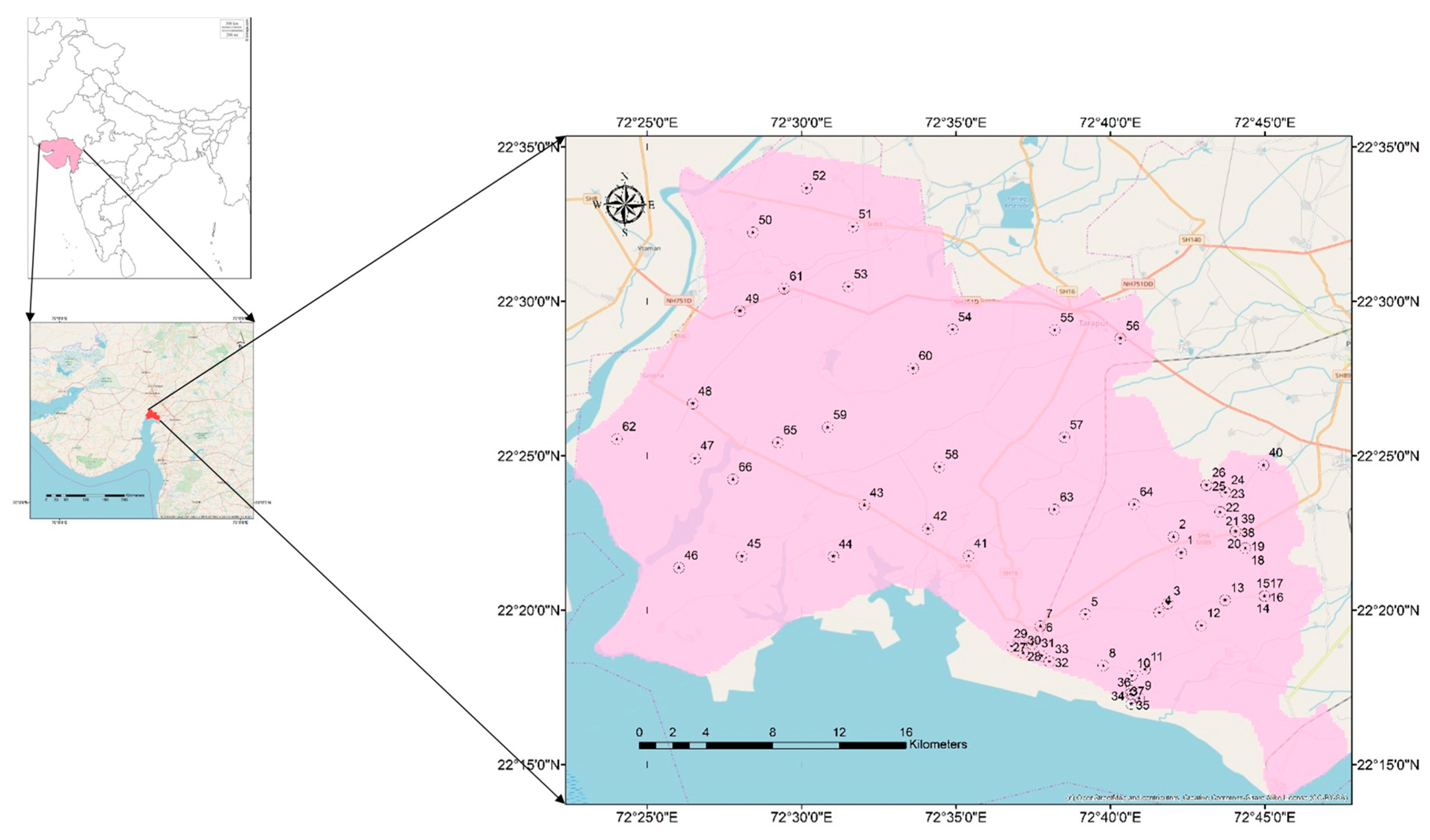
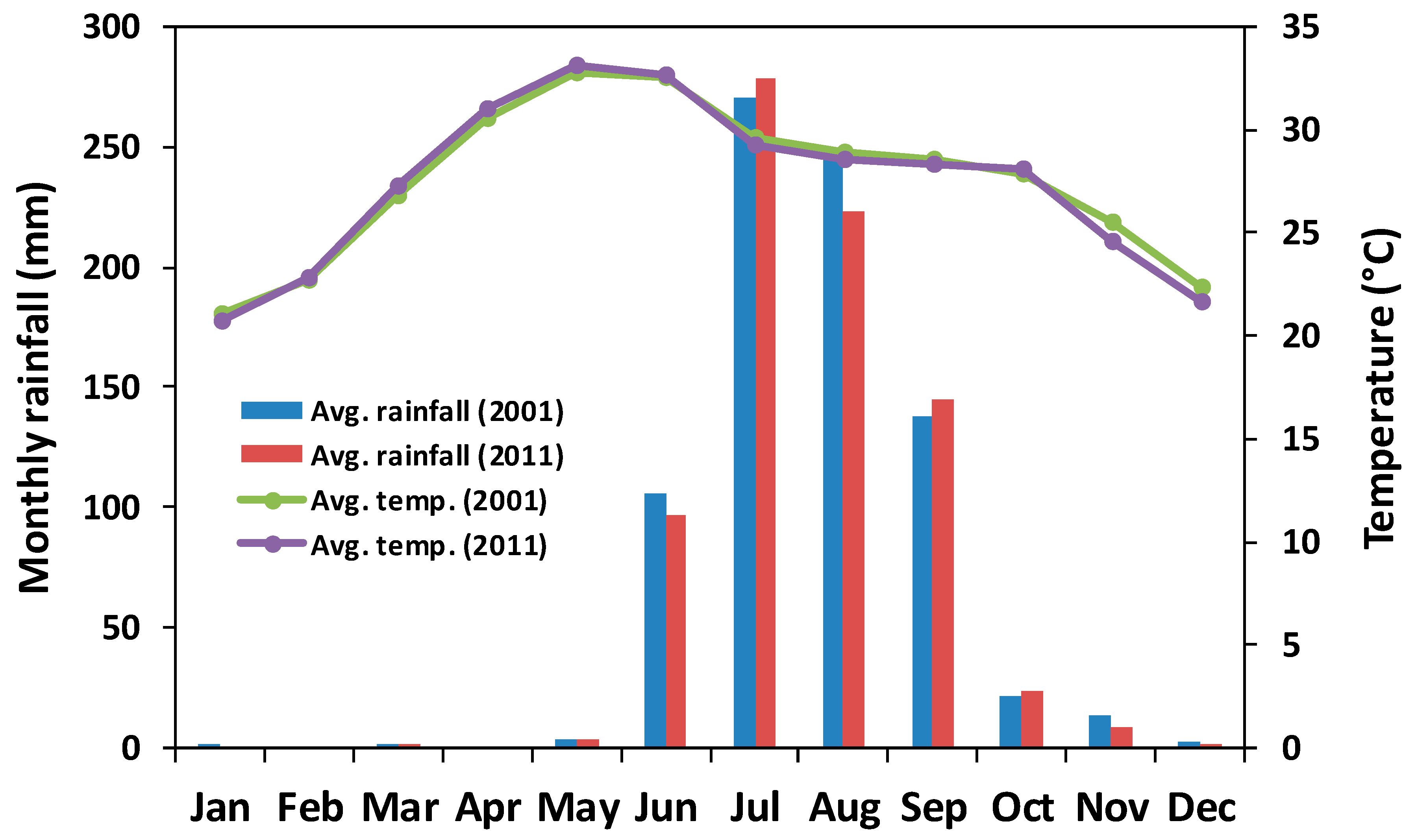
2. Study Area
3. Materials and Methods
3.1. Water Quality Analysis
3.2. Decadal Land Use Changes
3.3. Preparation of Contour Maps and Spatial Analysis of the Impacts of LU Changes of GW Quality
4. Results
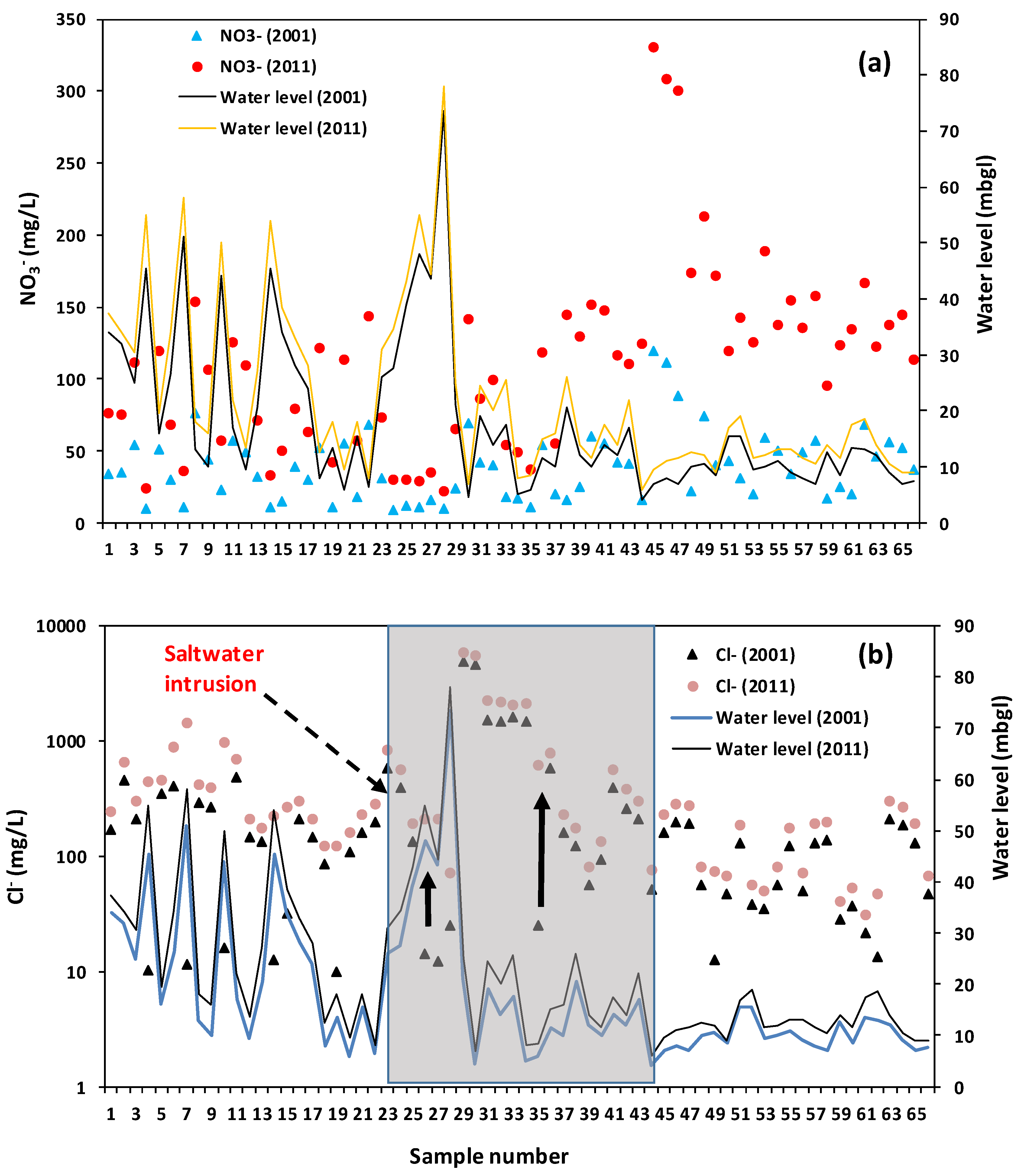
4.1. Water Quality Changes
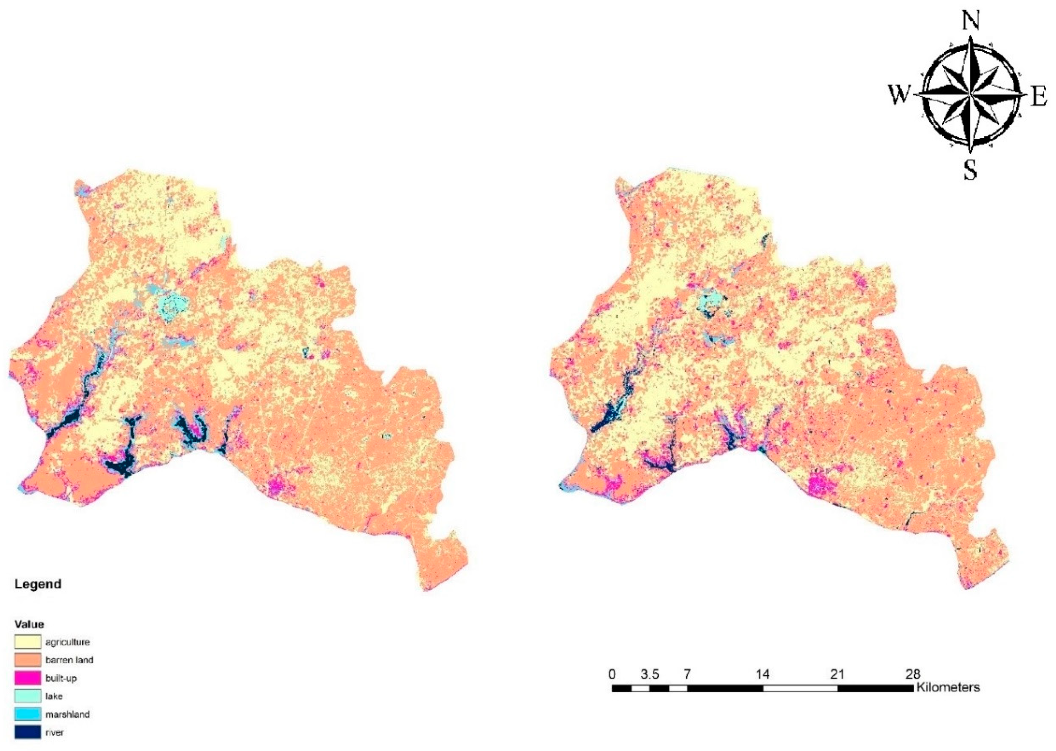
4.2. Land Use Changes
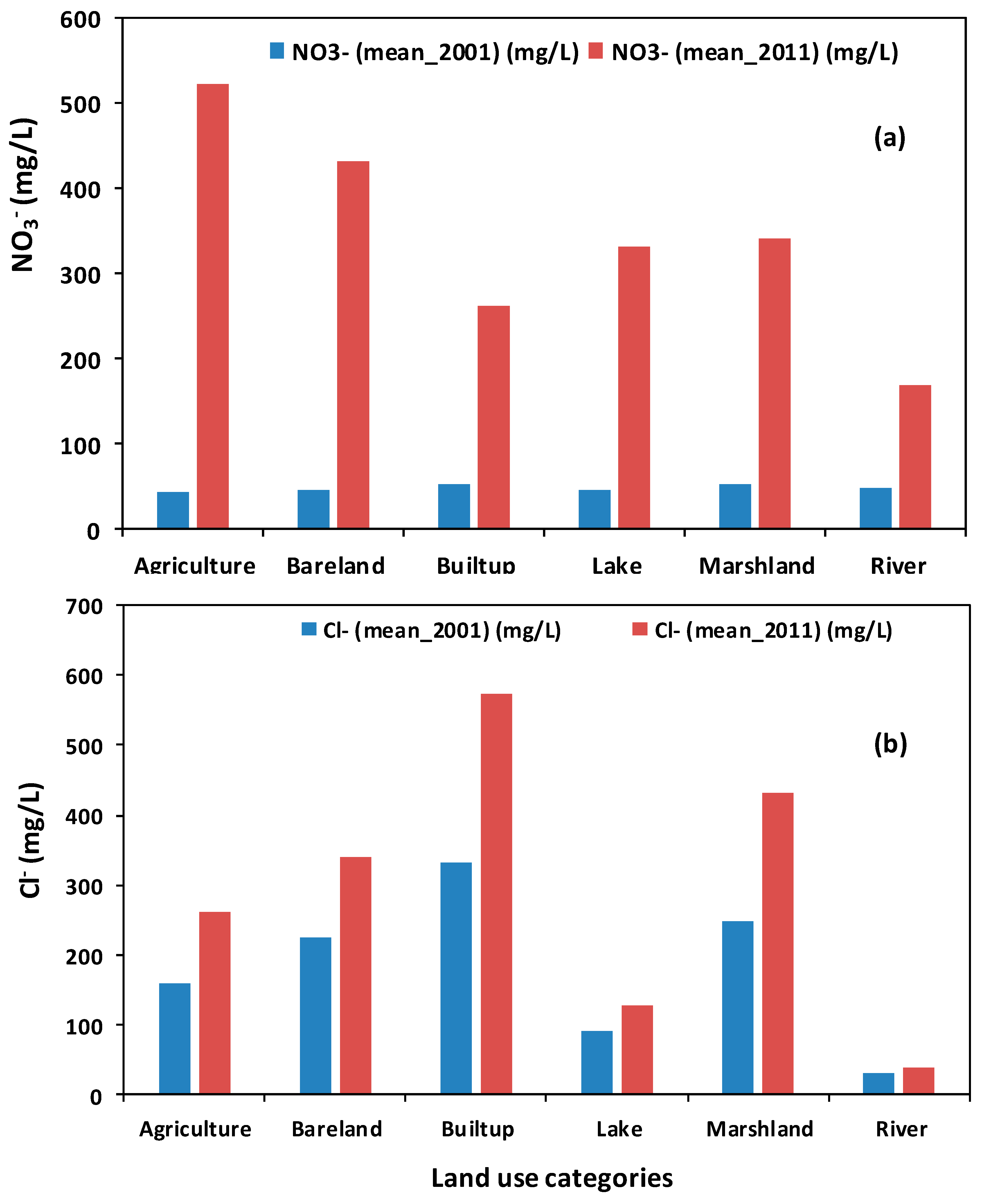
4.3. Relationship between Land Use Change and Water Quality
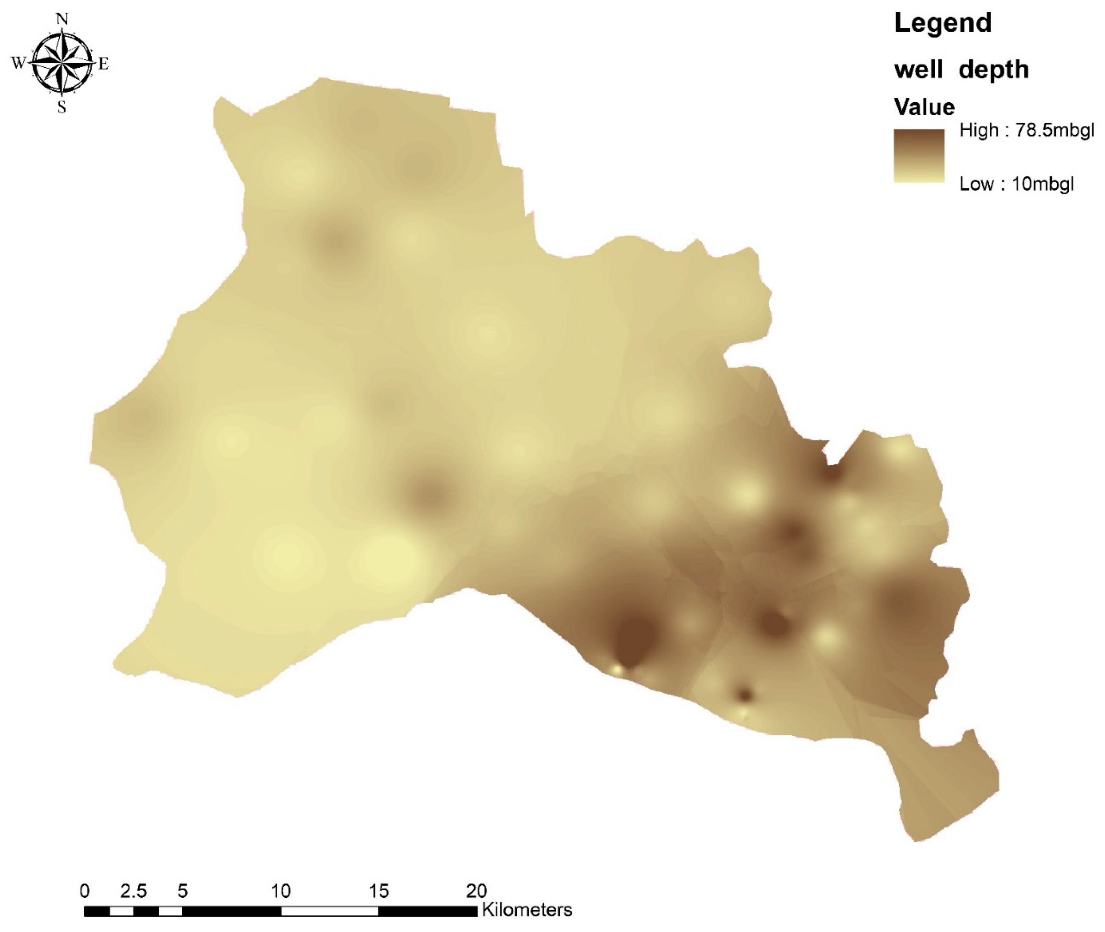
4.4. Zonal Statistics
5. Conclusions
Author Contributions
Conflicts of Interest
References
- Dabrowski, J.M.; De Klerk, L.P. An Assessment of the Impact of Different Land Use Activities on Water Quality in the Upper Olifants River Catchment. Water Sa 2013, 39, 231–241. [Google Scholar] [CrossRef]
- Saraswat, C.; Mishra, B.K.; Kumar, P. Integrated urban water management scenario modeling for sustainable water governance in Kathmandu Valley, Nepal. Sustain. Sci. 2017, 12, 1037–1053. [Google Scholar] [CrossRef]
- Chu, H.J.; Liu, C.; Wang, C. Identifying the Relationships Between Water Quality and Land Cover Changes in the Tseng-Wen Reservoir Watershed of Taiwan. Int. J. Environ. Res. Public Health 2013, 10, 478–489. [Google Scholar] [CrossRef]
- Gardner, K.K.; Vogel, R.M. Predicting Ground Water Nitrate Concentration from Land Use. Ground Water 2005, 43, 343–352. [Google Scholar] [CrossRef] [PubMed]
- Zeilhofer, P.; Lima, E.B.N.R.; Lima, G.A.R. Spatial patterns of water quality in the Cuiaba river basin, Central Brazil. Environ. Monit. Assess. 2006, 123, 41–62. [Google Scholar] [CrossRef] [PubMed]
- Ding, J.; Jiang, J.; Fu, L.; Liu, Q.; Peng, Q.; Kang, M. Impacts of Land Use on Surface Water Quality in a Subtropical River Basin: A Case Study of the Dongjiang River Basin, Southeastern China. J. Water 2015, 7, 4427–4445. [Google Scholar] [CrossRef] [Green Version]
- United Nation Sustainable Development Goals. The 2030 Agenda for Sustainable Development; A/RES/70/1; United Nation Sustainable Development Goals: New York, NY, USA, 2015; p. 41. [Google Scholar]
- Keesstra, S.; Mol, G.; de Leeuw, J.; Okx, J.; de Cleen, M.; Visser, S. Soil-related sustainable development goals: Four concepts to make land degradation neutrality and restoration work. Land 2018, 7, 133. [Google Scholar] [CrossRef]
- Steyl, G.; Dennis, I. Review of coastal-area aquifers in Africa. Hydrogeol. J. 2010, 18, 217–225. [Google Scholar] [CrossRef]
- Anderson, F.; Al-Thani, N. Effect of Sea Level Rise and Groundwater Withdrawal on Seawater Intrusion in the Gulf Coast Aquifer: Implications for Agriculture. J. Geosci. Environ. Prot. 2016, 4, 116–124. [Google Scholar] [CrossRef]
- Grundmann, J.; Khatri, A.A.; Schütze, N. Managing saltwater intrusion in coastal arid regions and its societal implications for agriculture. Proc. IAHS 2016, 373, 31–35. [Google Scholar] [CrossRef] [Green Version]
- Puckett, L. Nonpoint and Point Sources of Nitrogen in Major Watersheds of the United States; USGS Water Resources Investigations Report 94–4001; United States Geological Survey: Reston, VA, USA, 1994.
- Pérez-Fernández, M.A.; Calvo-Magro, E.; Valentine, A. Benefits of the symbiotic association of shrubby legumes for the rehabilitation of degraded soils under Mediterranean climatic conditions. Land Degrad. Dev. 2016, 27, 395–405. [Google Scholar] [CrossRef]
- WHO. Guidelines or Drinking-Water Quality, 4th ed.; World Health Organization: Geneva, Switzerland, 2011; p. 563. [Google Scholar]
- Bureau of Indian Standards (BIS). Indian Standard Drinking Water Specification, 2nd ed.; BIS 10500:2012; Bureau of Indian Standards: New Delhi, India, 2012.
- Manassaram, D.M.; Backer, L.C.; Messing, R.; Fleming, L.E.; Luke, B.; Monteilh, C.P. Nitrates in drinking water and methemoglobin levels in pregnancy: A longitudinal study. Environ. Health 2010, 9, 60. [Google Scholar] [CrossRef]
- Alfarrah, N.; Walraevens, K. Groundwater overexploitation and seawater intrusion in coastal areas of arid and semi-arid regions. Water 2018, 10, 143. [Google Scholar] [CrossRef]
- Kumar, P. Multi isotopic approach to study temporal variation of groundwater quality in coastal aquifer of Saijo Plain, Shikoku Island, Japan. Water Resour. 2013, 40, 208–216. [Google Scholar] [CrossRef]
- Hua, A.K. Land use land cover changes in detection of water quality: A study based on remote sensing and multivariate statistics. J. Environ. Public Health 2017, 2017, 7515130. [Google Scholar] [CrossRef]
- Huang, J.; Zhan, J.; Yan, H.; Wu, F.; Deng, X. Evaluation of the impacts of land use on water quality: A case study in the Chaohu Lake Basin. Sci. J. 2013, 2013, 329187. [Google Scholar] [CrossRef]
- Khan, A.; Khan, H.H.; Umar, R. Impact of land-use on groundwater quality: GIS-based study from an alluvial aquifer in the Western Ganges Basin. Appl. Water Sci. 2017, 7, 4593–4603. [Google Scholar] [CrossRef]
- Narany, T.S.; Aris, A.Z.; Sefie, A.; Keesstra, S. Detecting and predicting the impact of land use changes on groundwater quality, a case study in Northern Kelantan, Malaysia. Sci. Total Environ. 2017, 599–600, 844–853. [Google Scholar] [CrossRef]
- Persky, J.H. The Relation of Ground-Water Quality to Housing Density; USGS Water Resources Investigation Report 86-4093; USGS: Cape Cod, MA, USA, 1986.
- Kumar, P.; Kumar, A.; Singh, C.K.; Saraswat, C.; Avtar, R.; Ramanathan, A.L.; Herath, S. Hydrogeochemical Evolution and Appraisal of Groundwater Quality in Panna District, Central India. Expo. Health 2016, 8, 19–30. [Google Scholar] [CrossRef]
- Sarangi, R.K.; Chauhan, P.; Nayak, S.R. Inter-annual variability of phytoplankton blooms in the northern Arabian Sea during winter monsoon period (February-March) using IRS-P4 OCM data. Indian J. Mar. Sci. 2005, 34, 163–173. [Google Scholar]
- Kumar, N.; Kumar, P.; Basil, G.; Kumar, R.; Kharrazi, A.; Avtar, R. Chemo-metric analysis for evaluating geochemical processes responsible for spatio-temporal variation of surface water quality at Narmada estuarine region in Gujarat, India. Appl. Water Sci. 2015, 5, 261–270. [Google Scholar] [CrossRef]
- Central Ground Water Board (CGWB). District Groundwater Brochure; CGWB: Anand District, Gujarat, India, 2013; p. 20.
- Kumar, P.; Kumar, M.; Ramanathan, A.L.; Tsujimura, M. Tracing the factors responsible for arsenic enrichment in groundwater of the middle Gangetic Plain, India: A sourec identification perspective. Environ. Geochem. Health 2010, 32, 129–146. [Google Scholar] [CrossRef] [PubMed]
- Yen, S.T.; Liu, S.; Kolpin, D.W. Analysis of nitrate in near-surface aquifers in the Midcontinental United States: An application of the inverse hyperbolic sine Tobit model. Water Resour. Res. 1996, 32, 3003–3011. [Google Scholar] [CrossRef]


| Satellite/Sensor | Date of Pass | Path/Row | Spatial Resolution (m) | Band Considered with Spectral Resolution (μm) |
|---|---|---|---|---|
| Landsat-7 ETM+ | 10th November, 2001 | 148/45 | 30 | 0.45–0.52 (blue) |
| 30 | 0.52–0.60 (green) | |||
| 30 | 0.63–0.69 (red) | |||
| 30 | 0.77–0.90 (NIR) | |||
| Landsat-5 TM | 14th November, 2011 | 148/45 | 30 | 0.45–0.52 (blue) |
| 30 | 0.52–0.60 (green) | |||
| 30 | 0.63–0.69 (red) | |||
| 30 | 0.76–0.90 (NIR) |
| 2001 | 2011 | |||||
|---|---|---|---|---|---|---|
| Parameter | Range | Average | St Dev | Range | Average | St Dev |
| Well depth (mbgl) | 10.0–90.0 | 30.8 | 18.0 | 10.0–90.0 | 30.8 | 18.0 |
| Water level (mbgl) | 4.0–73.5 | 18.2 | 13.9 | 6.0–78.0 | 22.1 | 15.0 |
| pH | 6.8–7.8 | 7.3 | 0.3 | 6.4–7.7 | 7.4 | 0.5 |
| EC (µs/cm) | 362.0–8230.0 | 572.3 | 271.0 | 478.0–9792.0 | 837.8 | 415.0 |
| Na+ (mg/L) | 29.0–611.7 | 81.6 | 112.2 | 41.1–737.5 | 99.4 | 135.9 |
| K+ (mg/L) | 4.2–36.7 | 14.4 | 8.9 | 4.2–36.7 | 19.7 | 8.9 |
| Ca2+ (mg/L) | 13.8–251.6 | 101.2 | 10.1 | 40.2–303.7 | 138.0 | 34.7 |
| Mg2+ (mg/L) | 6.0–424.7 | 186.1 | 36.6 | 11.5–558.6 | 215.9 | 107.7 |
| HCO3− (mg/L) | 62.1–1032.3 | 156.5 | 135.6 | 68.2–1204.8 | 180.3 | 201.5 |
| SO42− (mg/L) | 13.3–234.8 | 42.4 | 25.7 | 20.0–366.7 | 63.3 | 76.1 |
| Cl− (mg/L) | 9.8–4874.9 | 375.1 | 862.6 | 31.0–5804.5 | 570.8 | 1004.3 |
| NO3− (mg/L) | 8.9–119.8 | 38.6 | 23.9 | 12.1–211.9 | 73.1 | 45.4 |
| PO43− (mg/L) | 1.3–44.1 | 3.9 | 5.6 | 5.4–78.6 | 5.7 | 20.2 |
| 2001 | 2011 | |||||
|---|---|---|---|---|---|---|
| LULC (Category) | Area (km2) | Proportion (%) | Area (km2) | Proportion (%) | Change in the Area | Change in Proportion (%) |
| Agriculture | 303.06 | 35.44 | 344.81 | 40.32 | 41.75 | 4.88 |
| Barren land | 465.64 | 54.45 | 429.45 | 50.21 | −36.19 | −4.23 |
| Built-up | 31.67 | 3.70 | 42.32 | 4.95 | 10.65 | 1.25 |
| Lake | 6.83 | 0.80 | 6.33 | 0.74 | −0.50 | −0.06 |
| Marshland | 33.87 | 3.96 | 18.96 | 2.22 | −14.91 | −1.74 |
| River | 14.18 | 1.66 | 13.37 | 1.56 | −0.81 | −0.09 |
| Agriculture | Barren Land | Built-Up | Lake | Marsh Land | River | Nitrate | Chloride | Water Level Reduction | |
|---|---|---|---|---|---|---|---|---|---|
| Agriculture | 1.00 | ||||||||
| Barren land | −0.78 | 1.00 | |||||||
| Built-up | 0.59 | −0.62 | 1.00 | ||||||
| Lake | 0.12 | 0.16 | 0.40 | 1.00 | |||||
| Marsh land | −0.51 | 0.20 | 0.37 | 0.03 | 1.00 | ||||
| River | −0.22 | −0.13 | 0.06 | 0.09 | 0.08 | 1.00 | |||
| Nitrate | 0.84 | −0.65 | 0.55 | 0.41 | −0.44 | 0.45 | 1.00 | ||
| Chloride | 0.47 | 0.33 | 0.17 | 0.12 | 0.67 | 0.36 | 0.24 | 1.00 | |
| Water level reduction | 0.79 | −0.45 | 0.88 | −0.23 | −0.31 | −0.28 | 0.66 | 0.80 | 1.00 |
© 2019 by the authors. Licensee MDPI, Basel, Switzerland. This article is an open access article distributed under the terms and conditions of the Creative Commons Attribution (CC BY) license (http://creativecommons.org/licenses/by/4.0/).
Share and Cite
Kumar, P.; Dasgupta, R.; Johnson, B.A.; Saraswat, C.; Basu, M.; Kefi, M.; Mishra, B.K. Effect of Land Use Changes on Water Quality in an Ephemeral Coastal Plain: Khambhat City, Gujarat, India. Water 2019, 11, 724. https://doi.org/10.3390/w11040724
Kumar P, Dasgupta R, Johnson BA, Saraswat C, Basu M, Kefi M, Mishra BK. Effect of Land Use Changes on Water Quality in an Ephemeral Coastal Plain: Khambhat City, Gujarat, India. Water. 2019; 11(4):724. https://doi.org/10.3390/w11040724
Chicago/Turabian StyleKumar, Pankaj, Rajarshi Dasgupta, Brian Alan Johnson, Chitresh Saraswat, Mrittika Basu, Mohamed Kefi, and Binaya Kumar Mishra. 2019. "Effect of Land Use Changes on Water Quality in an Ephemeral Coastal Plain: Khambhat City, Gujarat, India" Water 11, no. 4: 724. https://doi.org/10.3390/w11040724