Analysis of Shear Stress and Stream Power Spatial Distributions for Detection of Operational Problems in the Stare Miasto Reservoir


Department of Hydraulic and Sanitary Engineering, Poznan University of Life Sciences, ul. Wojska Polskiego 28, 60-637 Poznan, Poland
Water 2019, 11(4), 691; https://doi.org/10.3390/w11040691
Submission received: 8 March 2019
/
Revised: 28 March 2019
/
Accepted: 1 April 2019
/
Published: 4 April 2019
(This article belongs to the Special Issue The Application of Hydraulic and Sediment Transport Models in Fluvial Geomorphology)
Abstract
:In this paper an analysis of the lowland reservoir operation in atypical conditions is presented. The chosen study object is the Stare Miasto reservoir in the Powa river (Poland), which has been in operation since 2006. It is a two-stage reservoir, consisting of an upper sedimentation part and a lower main reservoir. The upper part is separated from the main part by an internal dam with a sluice gate. Such a construction enabled better control of sediment deposits and their removal. The atypical conditions were caused by flood wave propagation in the Powa river and the reservoir in 2014. In the research, three reservoir bathymetries are analyzed—from 2006, 2013, and 2018. Two-dimensional (2D) hydrodynamic modeling is applied to analyze spatial variability of investigated hydraulic parameters. Such an approach enabled better recognition of the changes observed in the reservoir during 2006–2018. In the research, the spatial distributions of the velocities, the shear stresses, and the stream power are the basis for the analyses and comparisons. The simulations enabled identification of the main elements prone to collapse during flood wave propagation. The presented results and approach may be applied for improvement of reservoir design, with special emphasis on specific structures located in a reservoir basin.
1. Introduction
This paper presents the problem of reservoir operation in the specific conditions of lowland areas. The paper focuses on special type of reservoir, whose construction has become rather popular. These are two-stage reservoirs, consisting of a preliminary sedimentation zone and a main zone. Only the main zone stores water for basic purposes of reservoir operation. The popularity of the two-stage reservoir is related to the fact that its construction reflects the nature of the reservoir sedimentation process. This feature simplifies removal of sediments without raising additional problems in the reservoir operation. Because in the past such solutions were not very popular and have become quite popular recently, the functioning of two-stage reservoirs is not understood at a satisfactory level.
The water resources in Poland compared to other European countries are relatively limited. Hence, it is important to build water reservoirs improving water balance, environmental water conditions, as well as microclimate. Typical reservoirs may be used for different purposes including drinking water supply, industrial water supply, and flood protection. Building reservoirs is economically profitable due to the production of electricity in water power plants. Reservoirs also may play an important role in tourism or as elements of the inland waterway.
The Wielkopolska (Great Poland) district is the region with the lowest rainfalls level in Poland. This is the reason why small retention is intensively developed in this area. There are 38 reservoirs classified as small retention objects. According to the Polish regulations, these are the reservoirs with storage smaller than 5 hm3. In Wielkopolska, there are also two large reservoirs with storage exceeding 5 hm3 [1]. The number of reservoirs indicates the significance of the discussed problem. Additionally, it is worth noting the economic importance of the reservoirs.
Operation of the water reservoir may cause several problems. In general, processes which are difficult to control occur in the reservoir and around it. Two problems are common for small and large reservoirs. These are, (1) erosion downstream of the reservoir dam, and (2) sediment deposition in the backward part of the inflowing river [2,3,4]. These processes occur relatively fast and cause a direct threat of reservoir catastrophe [3,5]. Although the processes occurring in the entire reservoir volume are also very important, they are slower and less visible in general [4,5,6,7]. The sediment transport in equilibrium conditions, occurring in the inflowing river, changes when water flows into the reservoir. The sediment transport potential rapidly decreases and the stream is not able to transport the same amount of sediments. Suspended and bed-loaded grains are deposited, creating alluvial fans and deltas in the inlet part of the reservoir. The density currents influence the water circulation in the reservoir. Finally, the fine sediments deposited in the deeper parts of the reservoir reduce the available volume and change the operational conditions in the longer time horizon [8,9,10,11,12]. In the inlet part of the reservoir, the deposition causes a decrease in the local depths and expansion of the riparian vegetation [6,13]. In two-stage reservoirs, these processes occur in the preliminary sedimentation zone. Water pollutants are also inhibited there, which improves water quality in the main part of the reservoir. However, pollutants are frequently deposited in the sediments (e.g., heavy metals) [14,15,16,17].
The object analyzed is the Stare Miasto reservoir, located in the Powa river in central Poland. This is a lowland reservoir with specific construction of the bottom. There is a preliminary zone separated from the rest of the reservoir by an internal dam. The flow between the upper and lower parts of the reservoir is limited. The upper part is usually smaller and plays the role of the initial sediment container, whereas the lower part is greater and it is designed to provide water for the main purpose of the reservoir operation. Hence, the lower part is usually called the main reservoir. There are basic reservoir capacities (i.e., active conservation storage, flood storage capacity, flood surcharge capacity, as well as dead storage). The described solution is one of the methods applied for prevention of sedimentation and water quality degradation in reservoirs [11,18,19]. Such an approach is not prohibitively expensive, though there are also some drawbacks. From the economic point of view, separation of the upper part means the loss of its conservation or flood storage. For this reason, broad research on such reservoirs, describing their operational conditions, seems worthwhile.
Taking into account the simplicity of the described concept, it is expected that such reservoirs will be built more frequently. In literature such objects have been rarely analyzed. Two other problems are discussed: (a) water and sediment quality [15,16,17,19,20]; (b) reservoir sedimentation [4,5,11,21,22,23]. These two processes make the described reservoir construction so attractive. Today a number of two-stage reservoirs in Poland can be found, for example, the Poraj reservoir in the Warta river, the Rydzyny reservoir in the Sama river, Kowalskie Lake in the Główna river, or the new concept of the Wielowieś Klasztorna reservoir in the Prosna river.
The basic feature of lowland reservoirs is very good vertical mixing of heat and dissolved substances. It means the lack of temperature stratification and uniform distribution of solutes along the depth. Due to the small depths, density currents caused by temperature and salinity gradients should not be present in such reservoirs. As reported by Krenkel et al. [24], the processes of heat and dissolved mass exchange in reservoirs without stratification vary in horizontal dimensions as in rivers.
Measurements and field surveys provide limited information on the spatial as well as temporal scale. The sampling techniques provide point information. Detailed description of the spatial distributions of investigated parameters (e.g., velocities, temperature, etc.) requires a huge number of such measurements and, obviously, it is time-consuming and expensive. A similar problem arises when the temporal variability of the selected parameters is formulated. The duration of the analyzed processes is important. The description of their dynamics requires continuous measurements or very frequent momentary measurements. Hence, the application of mathematical modeling in the analysis may help. Different types of models for description of river and reservoir dynamics have been applied for many years. One-dimensional (1D) unsteady flow models are the simplest models applied for reservoirs [25,26]. However, models of this kind are able to reconstruct properly only the variability of the depth in the reservoir. Other hydraulic parameters (e.g., velocities, shear stress, etc.) are determined approximately. Modeling of other processes in 1D mode for reservoirs is burdened with significant inaccuracies. Because of this, 2D and 3D modeling is more frequently used for analysis of reservoirs. In the lowland reservoir, 2D models are preferred due to relatively small depths [25,27,28,29,30]. Such an approach enables determination of quite accurate spatial distributions of basic hydraulic variables (e.g., depth and velocity) and parameters dependent on their values (e.g., shear stress, stream power, and others) [29,30]. More accurate reconstruction of the hydraulic variables range is also the basis for modeling of other processes (e.g., transport of pollutants or sediment transport). The field measurements impact the construction of the model during the procedure of identification and verification. The final product is a model giving results (e.g., depth, velocities, etc.), consistent with observations in the field. It may be applied for test computations and forecasting. Such a model may support analysis of spatial and temporal variability of the investigated variables.
The purpose of the present research is to analyze two-stage reservoir operation, with its hydraulic and operational problems. The presented approach is based on the 2D simulations of a hydrodynamic model made for a flood scenario selected from historical data. The flood wave observed between 10 April and 19 July of 2014 is used. The attention is focused on three variables identified as the measures of potential hazards: (1) magnitude of flow velocity, (2) shear stress, and (3) stream power. The role of the flow velocity in morphodynamical changes in rivers and reservoirs is well known. Such processes as sediment deposition and erosion are observed in locations of significant velocity changes (e.g., reservoir inlets, contractions in channels, etc.). The shear stress describes these processes better with the so-called incipient motion criteria. In such objects as reservoirs, the shear stresses have specific distributions, and they may be concentrated near hydraulic obstacles (e.g., dams and bridge piers). The stream power is a combination of velocity and shear stress, with potential to link the features of both variables. Hence the stream power is a basis of many sediment transport formulae applied for modeling of sediment deposition and erosion in rivers and reservoirs. The spatial distributions of these variables are confronted with the known locations of threats (e.g., internal dam almost crashed in 2014). The main assumption is that the careful analysis of such spatial distributions may help to prevent undesirable threats in the stage of reservoir design. The analyses are made for three bathymetries reconstructed for the years 2006, 2013, and 2018. The comparison of velocity, shear stress, and stream power distributions in these three moments of time could help to understand better the nature of processes responsible for morphodynamic changes in the reservoir.
2. Case Study System
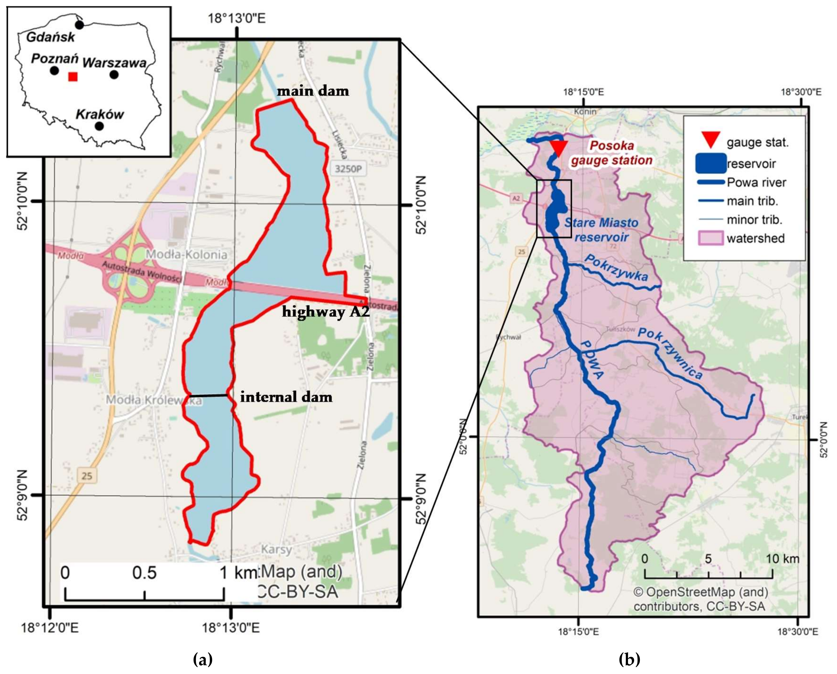
Taking into account the purpose of the research, quite a specific object, the Stare Miasto reservoir in the Powa river, was chosen as a case study. The Powa is a moderately sized river flowing in the lowland of Great Poland province in the central part of Poland. The Stare Miasto reservoir was built as an element of the small retention program [31]. The purposes of this program are the improvement of watershed capacity, flood and drought protection, and prevention of a decrease in the groundwater table. The analyzed reservoir has been in operation since 2006. It is divided into two parts (Figure 1), with an internal dam located at km 12 + 000 of the Powa river. There is a regulated sluice applied to control flow through the dam. The upper zone works as a sediment trap.
The inundation area of the upper part is 27 ha and its storage equals 0.294 hm3. The lower part is the so-called main reservoir. This part is additionally split into two internal parts by highway A2 (Figure 1), running from Poznań to Warsaw [32]. The watershed area of the Stare Miasto reservoir in the cross-section of the main dam is 299.7 km2. The average depth of the reservoir is 2.4 m. The estimated length of this object is 4.5 km. The inundation area for the minimum headwater level (MinPP = 92.0 m a.s.l.) is 75.77 ha. For the normal headwater level (NPP = 93.5 m a.s.l.) the inundation area is 90.68 ha. The maximum headwater level (MaxPP) is 94.0 m a.s.l. The total reservoir capacity is 2.159 hm3. The active conservation storage is 1.216 hm3. The inundation area of the upper zone is 13.62% of the total water surface area. The land use in the neighborhood of the reservoir agriculture. Because the usefulness of the terrain is limited, crop production has been stopped in this region [32,33]. The reservoir is working in an annual compensation cycle, which may cause annual variation in the water level, from MinPP to NPP. The operational water level is from 92.00 m a.s.l. to 94.00 m a.s.l. The reservoir is filled in March and the water surface is kept at the level of NPP until the end of October. After October, the main reservoir is emptied to the level of MinPP. To protect the inlet part from degradation and sediment accumulation, the water surface in the upper part is kept at the NPP level for the entire year.
In the Powa river there is one gauge station called Posoka (Figure 1b). This is located downstream of the reservoir at km 3 + 900 of the Powa course. The watershed area in the cross-section of the gauge is 332 km2. The characteristic flows were determined on the basis of recorded observations at this gauge station during the period 1975–2017 [34]. The results are presented in Figure 2. The total minimum observed was 0.006 m3/s, while the total maximum was 42.6 m3/s. The mean flow was about 1.15 m3/s. During the time of reservoir operation, from 2006 to 2017, the maximum flow of 28.5 m3/s (Figure 2b) occurred in 2014. The minimum and mean flows did not differ much from those estimated for the entire period. In the analyzed period, the average annual outflow from the reservoir was 36.9 hm3.
Operational Problems in the Reservoir
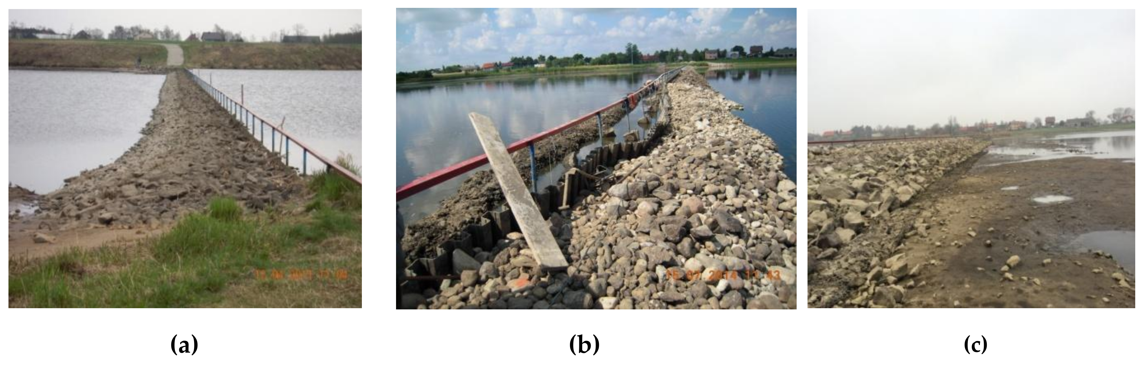
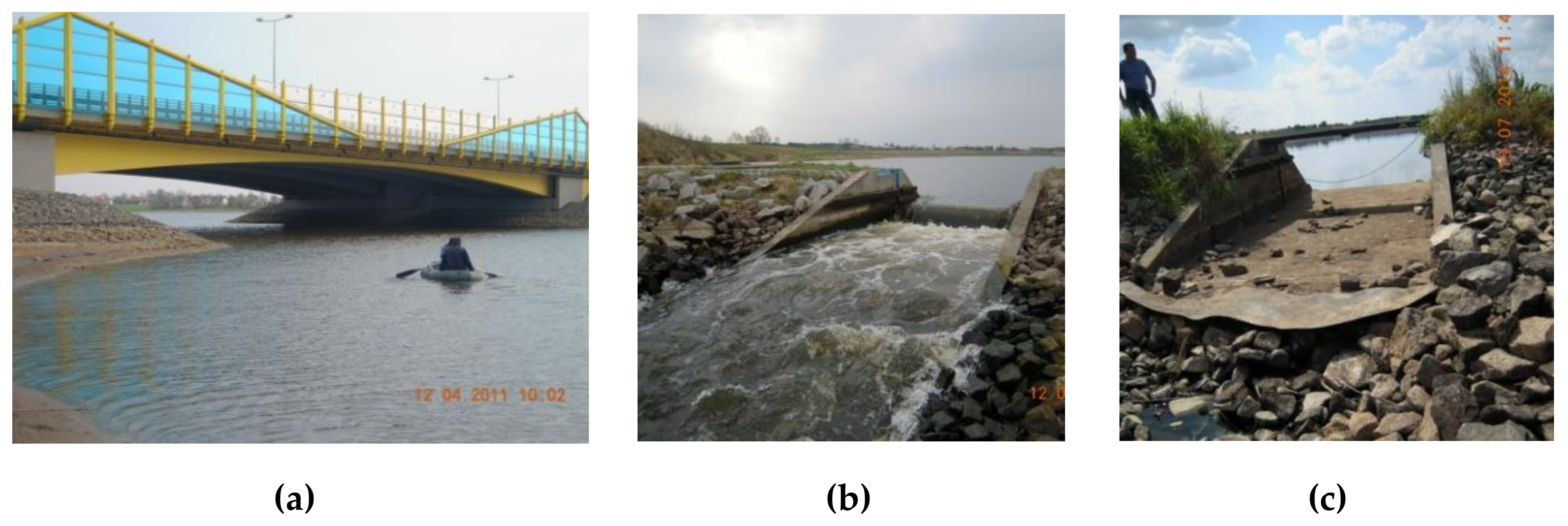
Operational problems have been present in the Stare Miasto reservoir since its construction. The first of them is caused by the internal dam splitting the reservoir into two parts. As mentioned above, the headwater level should be constant over the entire year (Figure 3a–c). The flow through the internal dam from the preliminary sedimentation zone to the main part of the reservoir is regulated by the sluice installed in the internal dam (Figure 4b,c). Due to the internal dam instability and the too small span of the sluice, equal to 3 m, the sluice was totally opened almost all the year. The problems with the internal dam increased in 2014, when huge flows in the Powa river occurred (Figure 4b) after heavy rainfalls in the upper watershed, which caused local flooding.
High water stages and a fast-flowing flood wave reached the reservoir and met the internal dam. Due to the huge force acting on the dam during the flood wave propagation in 2014, the structure was damaged (Figure 3b).
In 2014, it was decided that the internal dam would be reconstructed and the sediments would be removed from the upper part of the reservoir. The construction works were carried out in 2015. In the upper part the layer of sediments from the reservoir bottom was removed. The depth of the layer was 40 cm. The area of removal covered about 2 ha and the estimated volume of the removed sediments was 8000 m3. The soil removed was distributed more or less uniformly along the banks. The sluice gate was reconstructed in such a way that inverted elevation was decreased.
3. Materials and Methods
3.1. Available Data
In the research four types of data were applied: (1) Hydrologic data for the Posoka gauge station; (2) the measurements of reservoir bathymetry made in 2006, 2013, and 2018; (3) a digital elevation model (DEM); and (4) sediment samples collected in 2011 and 2018.
The hydrological data for the Posoka gauge station were obtained from the Institute of Meteorology and Water Management (IMGW—Polish: Instytut Meteorologii i Gospodarki Wodnej). Although the available daily data was for the period 1971–2017 (Figure 2), the single flood wave observed between 10 April and 19 July of 2014 was used for simulations. The DEM applied in this research was obtained from the Head Office of Geodesy and Cartography (GUGiK—Polish Główny Urząd Geodezji i Kartografii). Its spatial resolution was 1 × 1 m. The vertical accuracy was 15 cm.
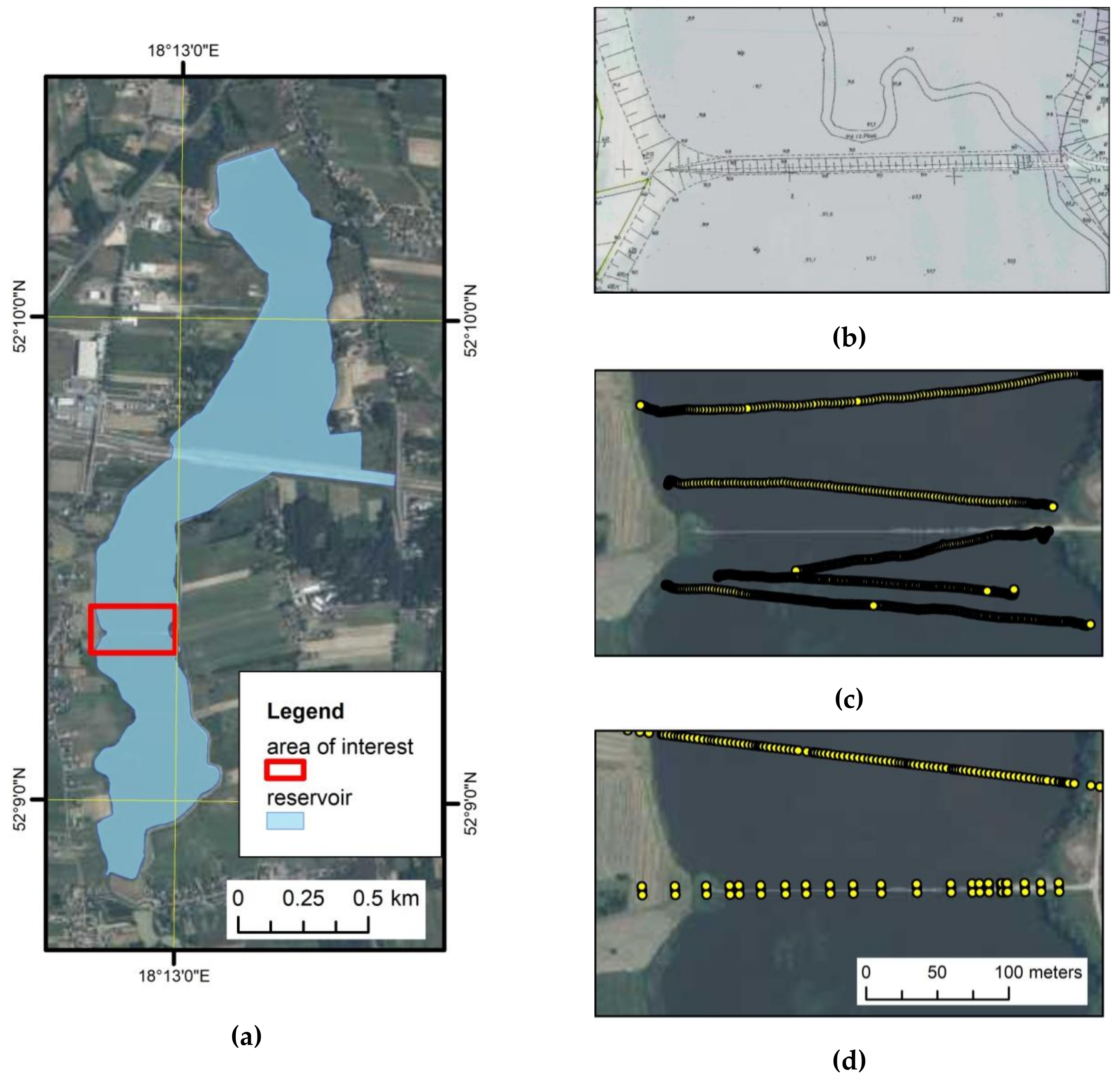
Examples of the data applied to create a computer model of bathymetries are presented in Figure 5. Figure 5a shows the reservoir shape and the location of the area for presentation of details. This area was chosen as a part of the reservoir near the internal dam. The bathymetry reflecting the year 2006 was reconstructed on the basis of topographic maps used for the reservoir design purposes (Figure 5b). The digital elevation model was built on the basis of elevations and isolines presented in the maps. In 2013, the bathymetry of the reservoir was measured in cross-sections with two devices: (1) GPS; and (2) an Echotrac CVM depth sounder. The total number of cross-sections was 98 and the distances between them varied from 50 to 100 m. Examples of these data is shown in Figure 5c. The last bathymetry was measured in 2018 as a part of the ISOK project (Polish: ISOK = Informatyczny System Osłony Kraju przed nadzwyczajnymi zagrożeniami, English: IT system of the Country’s Protection Against Extreme Hazards). The second part of the project started in 2017 and the data from this part were applied for the presented research. The total number of cross-sections was 14 and the distances between them were in the range 200–300 m. Measurement points locations are shown in Figure 5d.
The last set of data applied in the research included sediment samples measured in 2011 and 2018. In 2011, 36 sediment samples were collected. In 2018 the measurements were repeated and 30 samples were taken from the reservoir bottom. The granulation based on 66 samples measured in 2011 and 2018 was determined as a combination of sieve and aerometer analysis, according to Polish norm PN-R-04032:1998 "Soils and minerals—samples and analysis of granulation." The sieve analysis was performed in wet conditions with a normalized set of sieves. The aerometric analysis was performed with a set of aerometric devices produced by Eijkelkamp. According to the above-mentioned Polish norm, the soil fractions taken into account were as follows: sand (2–0.05 mm), silt (0.05–0.002 mm), and clay (0.002 mm).
3.2. Applied Methods
The ArcGIS 10.5.1 software developed by Esri Inc. was applied which is described in e.g., Docan [35]. It enables quite easy processing of GIS data, such as vector and raster layers. An integral part of ArcGIS is the ArcToolbox. It is a module including the main external tools and methods. Some of them are concurrent to the methods available in the basic ArcGIS interface, while others extend the capabilities of the standard interface. Extension of ArcGIS is also possible with specific plug-ins installed as ArcGIS toolbars. One such plug-in is HEC-GeoRAS [36], which is a toolbar with methods designed to support preparation of the river flow model. The tools available in HEC-GeoRAS may also be useful in preparation of a 2D model for simulation of flow in a reservoir.
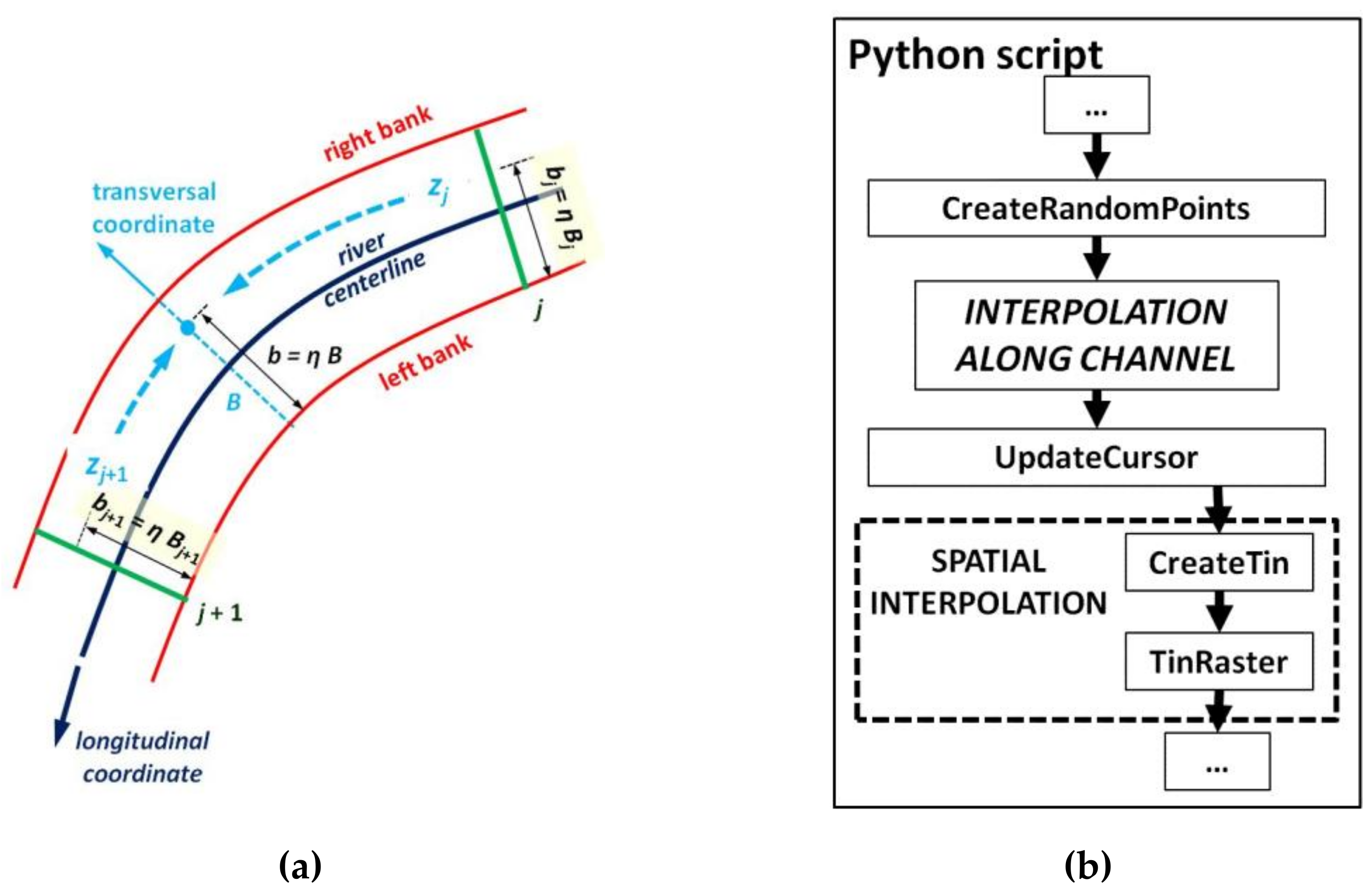
The second plug-in applied is RiverBox, which is a set of geo-processing tools developed in Python by Dysarz [37]. Although the software was designed primarily for reconstruction of a river bed, after preliminary data processing it has been also successfully applied for this reservoir. The basic idea of interpolation in the channel-oriented coordinates is shown in Figure 6a. The bottom elevations are reconstructed from measurement cross-sections (green lines) through linear interpolation in two directions: the longitudinal and the transversal. The plug-in includes a number of algorithms for measurement data processing and three algorithms for reconstruction of the bed. These are described in more detail in the quoted publication [37]. The scheme of the third algorithm applied here is presented in Figure 6b. The main idea was to create a number of random points over the interpolated area, channel-oriented interpolation of the elevations in the points, and finally application of “typical” spatial interpolation. In the third algorithm of the RiverBox, the linear interpolation in the two dimensions was applied for this purpose. It wa implemented by adoption of two tools from ArcToollbox: creation of TIN (Triangular Irregular Network) and transformation of the TIN into standard raster. The choice of the third algorithm was determined by its effectiveness analyzed in Dysarz [37].
Three bathymetries of the analyzed reservoir were reconstructed from available data, they represent the reservoir bed from 2006, 2013, and 2018. The first was composed from detailed design maps of the reservoir, with application of geo-referencing and digitization. The next two were reconstructed with the help of the RiverBox plug-in for ArcGIS Desktop software.
The HEC-RAS is a well-known hydrodynamic model for rivers and water reservoirs. This program was designed at the Hydrologic Engineering Center (HEC). The acronym RAS means River Analysis System, which well defines the application area. The concepts applied in the package are described by [38]. The main features of HEC-RAS are 1D simulations of flow and transport processes in river networks, including floodplains and reservoirs, as well as 2D simulations of pure flow. The HEC-RAS package also includes several useful tools for data preparation and results processing. These tools include the module for GIS data processing called RAS Mapper [39].
The 2D flow module was applied in this research. The basic model for such simulations implemented in HEC-RAS is the full dynamic wave [38] presented below
where the Equation (1) describes mass balance and the next two, Equations (2) and (3), are momentum balance equations. The independent variables are —time and , —spatial dimensions. There are three dependent variables, namely —the water depth, and , —the depth-averaged components of flow velocity. The water surface elevation depends on the depth and is acceleration of gravity. There are also two coefficients of more complex nature. The first is kinematic eddy viscosity coefficient defined as follows
where is non-dimensional empirical constant describing mixing intensity and is well known shear velocity. The second coefficient is bottom friction coefficient derived from Chezy or Manning formulae as follows
where is hydraulic radius and is magnitude of velocity vector. There are also velocity coefficient for Chezy equation and roughness coefficient for Manning equation .
The interpretation of mass balance in Equation (1) is relatively simple. In arbitrary control volume, the inflow and outflow fluxes described by the second and third terms of the equation should be in balance with the increase or decrease in the water volume stored, which is expressed in terms of water surface elevation changes in the first term. The left sides of Equations (2) and (3) describe the change in the momentum stored in the control volume, including the momentum stored locally and the momentum fluxes. The first terms of the right sides represent the pressure and gravity forces, while the second is responsible for internal eddy stresses and mixing. The last terms of the right sides describe the friction force generated on the contact surface of the liquid and bottom.
In HEC-RAS, the simulation may be performed with a simplified version of the model (1)–(3). If the left side of momentum equations and the eddy viscosity terms are neglected, the model (1)–(3) becomes the so-called diffusive wave model [38].
In the above equation plays a role of diffusion coefficient and it is defined as
where is the magnitude of water surface gradient or, in other words, the water surface slope. The model (6) with (7) is the default choice due to stability and efficiency. The simulations presented here were performed with the diffusive wave model.
The equations are approximated with a hybrid scheme based on a combination of finite difference and finite volume methods. Such an approach is applied due to the fact that the computations mesh is composed of rectangular elements inside the flow domain and multi-edge irregular elements near the boundaries [38]. The applied boundary conditions are a flow hydrograph in the reservoir inlet and a constant stage hydrograph in the reservoir outlet.
The obtained results were transformed into the cell-oriented shear stress and stream power values. These two variables are defined as follows
where is energy grade line slope (friction slope).
For the purposes of the present research, three models were developed. All of them were 2D models of the entire reservoir. Elements such as the bridge, internal dam, and main dam were reconstructed by modification of elevations in a digital terrain model representing the reservoir bottom. The basis for the 2D simulations was the numerical mesh covering the entire reservoir area, approximately equaling 1 km2. The imposed cell size of rectangular cells was 2 × 2 m, but the cells near the boundaries may have different shapes. Hence, the minimum cell area was 1.74 m2 and maximum was 7.87 m2, when the total average was 4.01 m2. The total number of cells covering the reservoir was 241,699. Three bottoms were tested, which were the reconstructions of the real reservoir for 2006, 2013, and 2018. The reconstruction process is described above. In all cases the flood wave observed in 2014 was simulated with constant head water kept in the reservoir outlet. The elevation of the head water simulated was 93.50 m a.s.l. This is the so-called normal head water level in the Stare Miasto reservoir. The simulation time step was chosen due to the stability requirements and it equaled 30 s. Because the semi-implicit scheme was used for time discretization, the weighting factor was set to 0.75.
Besides the geometry reconstruction and flow boundary conditions, the important elements determining the flow process in the analyzed area were roughness coefficients. A simplified approach was used for this purpose. The sediment samples collected from the reservoir bottom were the basis for determination of the equivalent roughness coefficient for the entire reservoir bottom. Two step calculations were applied. In the first step, the dimensionless resistance coefficient λ from the Darcy–Weisbach formula was determined for full turbulent flow conditions:
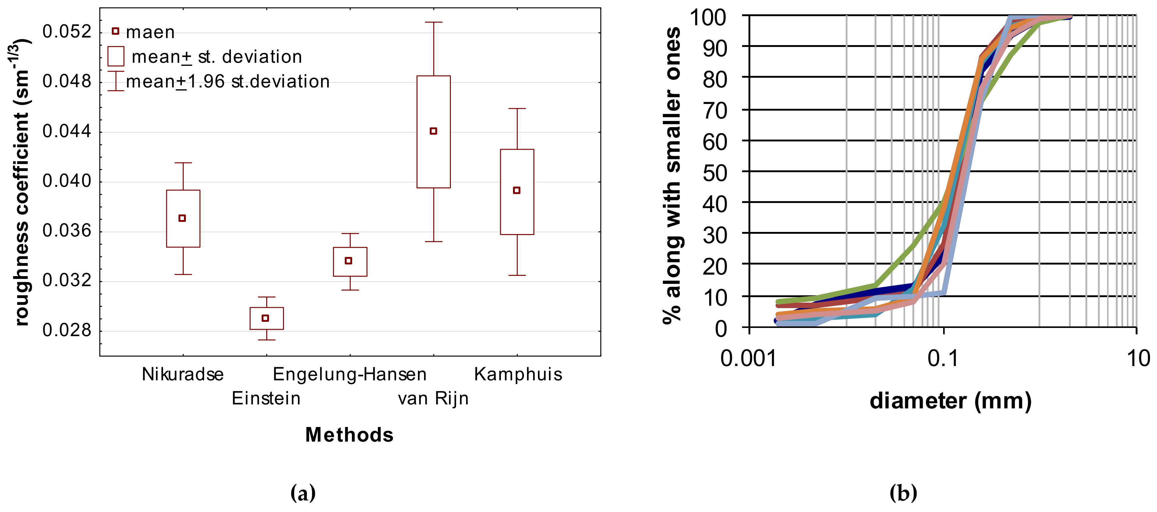
where Rh is the hydraulic radius and ks is the absolute roughness. The second coefficient was defined theoretically as the average height of bottom irregularities. In practice its value was calculated on the basis of sediment characteristics, but a number of formulae have been proposed in literature for this purpose. The chosen and applied approaches are presented in Table 1 [40]. The symbol dx in this table means specific diameter of the grain sample determined on the basis of the sieve curve. The next step was calculation of Manning’s roughness coefficient n from the formula:
In Figure 7a, the box-and-whiskers plot, representing the relationship between the five methods listed in Table 1 and the roughness coefficients, is presented. The sediment characteristics were determined on the basis of the 66 sieve curves obtained from sediment samples, presented in Figure 7b, in which dots represent the mean values. The boxes show the values of the mean ± standard deviation. The whiskers denote the values between mean ± 1.96 standard deviations, which define the 95% confidence level. The plot presented in Figure 7a summarizes 330 calculations of roughness coefficients. The obtained average value was 0.038 sm−1/3, while the minimum and maximum values were 0.026 and 0.059 sm−1/3, respectively.
4. Results and Discussion
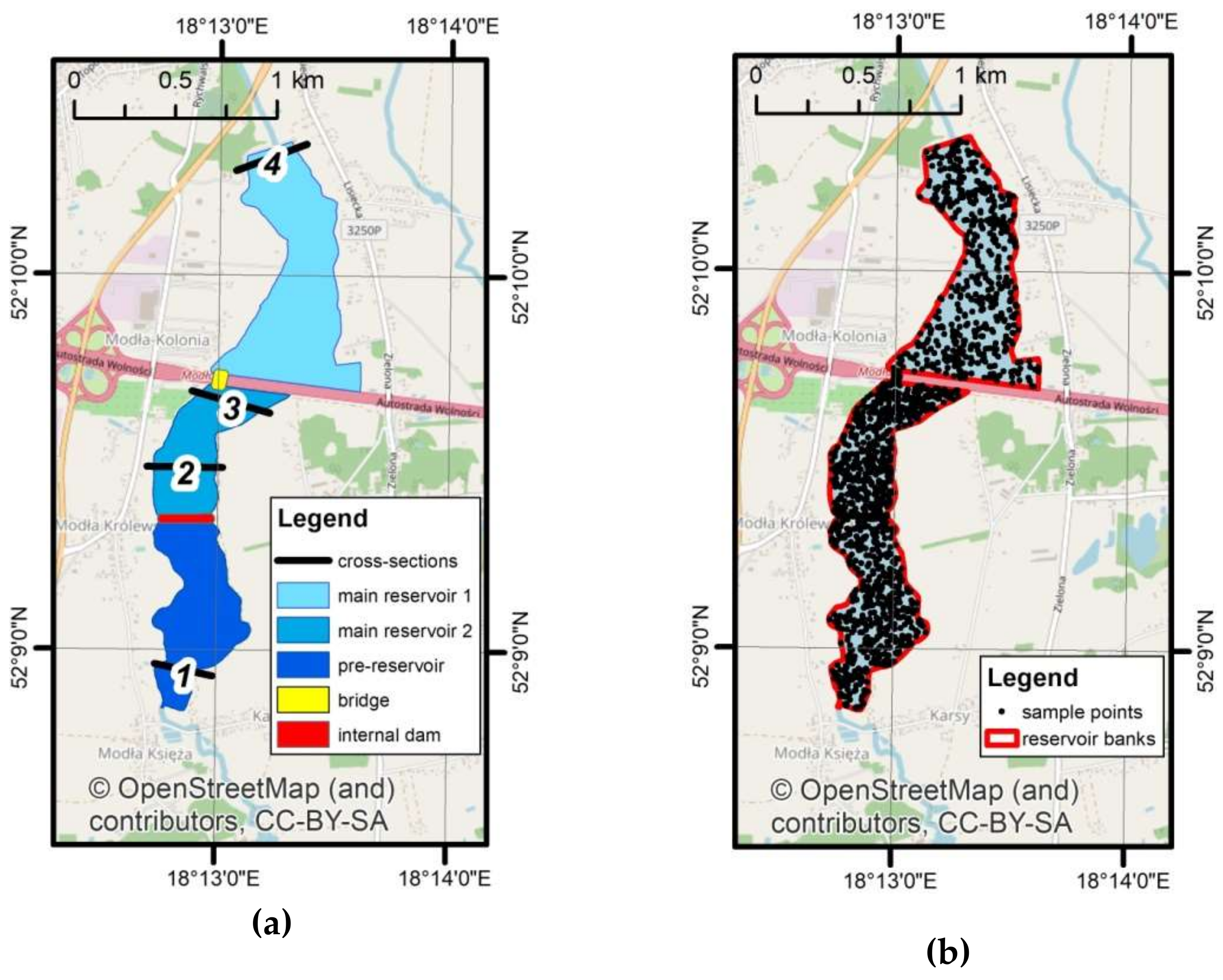
On the basis of 2D simulations, the depths, flow velocities, shear stresses, and stream power were determined for the entire reservoir with each of the three different bathymetries. Due to the huge amount of data, the results were kept in three groups: maps, graphs of selected cross-sections, and graphs with statistical analyses. In Figure 8, the locations of the main elements applied to analyze the results is shown. The reservoir was divided into five parts as presented in Figure 8a. They were, (1) the main reservoir 1, (2) the main reservoir 2, (3) pre-reservoir, (4) area under bridge, and (5) the internal dam. The four cross-sections were located in characteristic places of the greatest parts. There was 241,699 computational cells in the numerical grid. Because this number of cells was difficult for processing, the sample points (Figure 8b) were used for monitoring the obtained results. The total number of sample points was 1670, which was about 0.67% of the available locations of computed values. Although this number was much smaller than the number of computational cells, the sample points covered the entire reservoir with sufficient density. Because the reservoir parts differed in size, their distribution over the parts was not uniform. In the main reservoir 1, the main reservoir 2, and pre-reservoir there were 500 points, while 20 points were generated in the area under the bridge and 150 points generated over the internal dam.
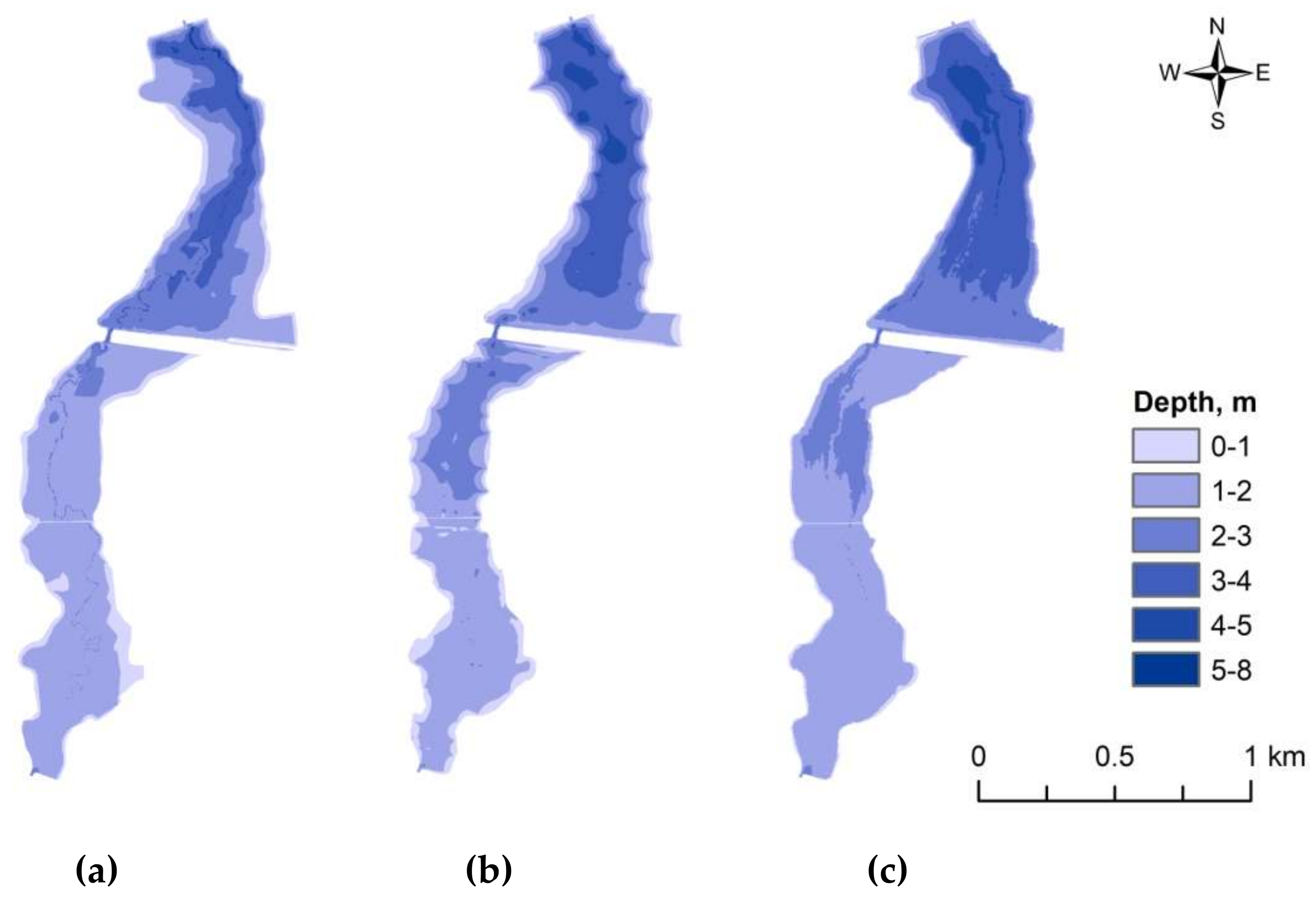
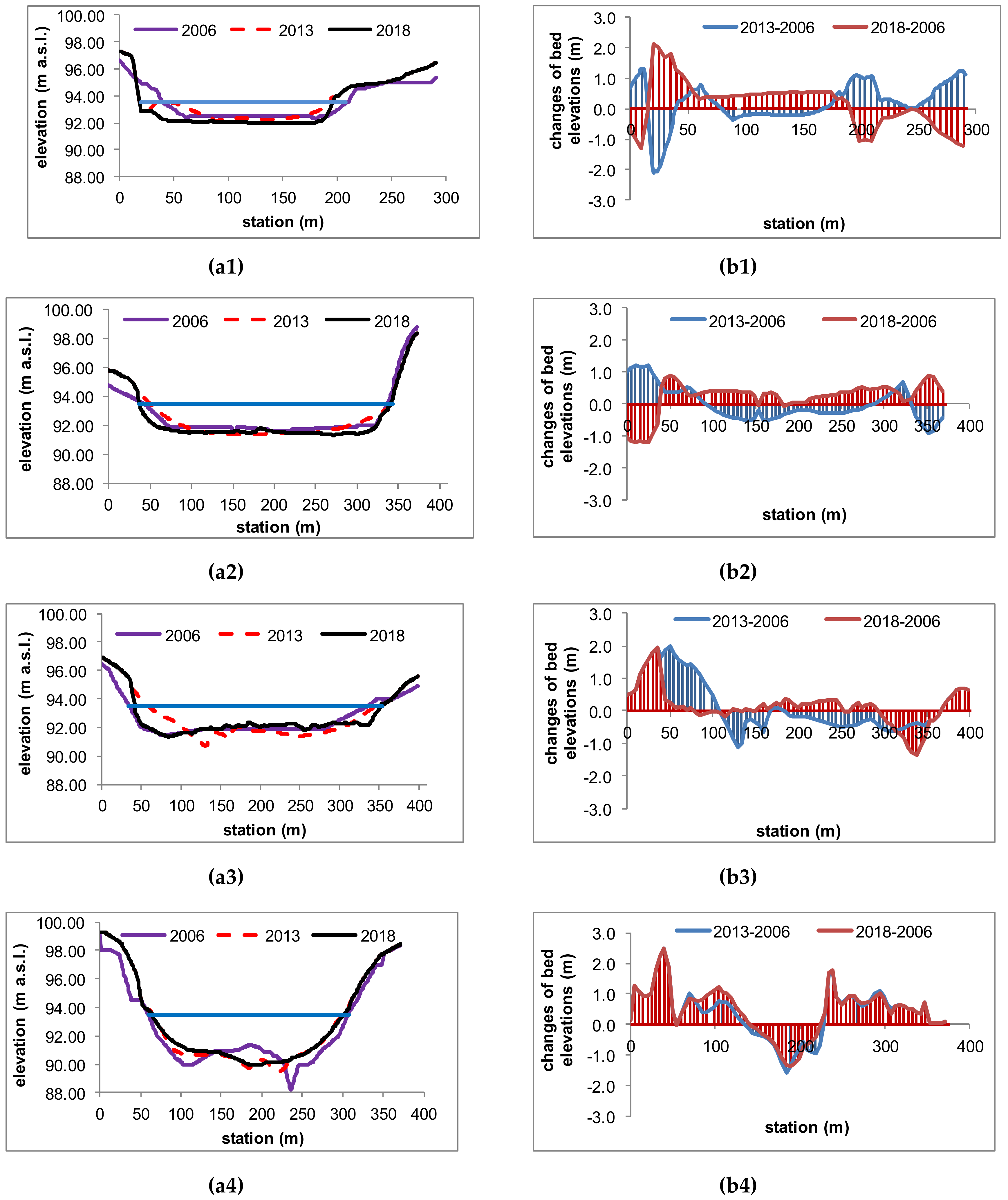
The maps presented in Figure 9, Figure 11, and Figure 12 show the spatial distribution of depth, velocity, and shear stress over the three reservoir bathymetries, namely 2006, 2013, and 2018. As may be observed, the reservoir bottom changed during 12 years. Figure 9 presents the maps of maximum depths obtained as the results of simulations. The following maps (Figure 9a–c) show the results for bathymetries of 2006, 2013, and 2018, respectively. The comparison of bathymetries is made in Figure 10—part A (Figure 10(a1–a4)), where the geometry of cross-sections marked in Figure 8 is shown. In part B of Figure 10 (Figure 10(b1–b4)), the differences of the bottom elevations related to the initial bathymetry 2006 were analyzed. The blue line denotes increase in the elevations, from the initial bathymetry to the bathymetry measurement in 2013. The red lines represent differences between measurements of 2018 and the initial data.
As it can be seen, during the life of the reservoir, since 2006, the reservoir bottom was considerably transformed. Figure 10, graph b1 shows the cross-section located in the inlet of the Stare Miasto reservoir. The differences in the bottom elevations varied from 2 m of accumulated sediments to 2 m of removed sediments. The comparison with the bathymetry of 2006 shows that the greatest differences occurred in 2018 as a result of natural processes, as well as artificial removal of sediments in the end of 2014 and the beginning of 2015. At this time, a 0.4-m layer of sediments was removed from the bottom of the upper part. Figure 10(b2,b3) show similar bottom increases for the bathymetries of 2018 and 2006. In the last cross-section located near the main dam, the sediments were accumulated during 12 years of reservoir life. The only place where erosion occurred was located near the valve tower and spillway.
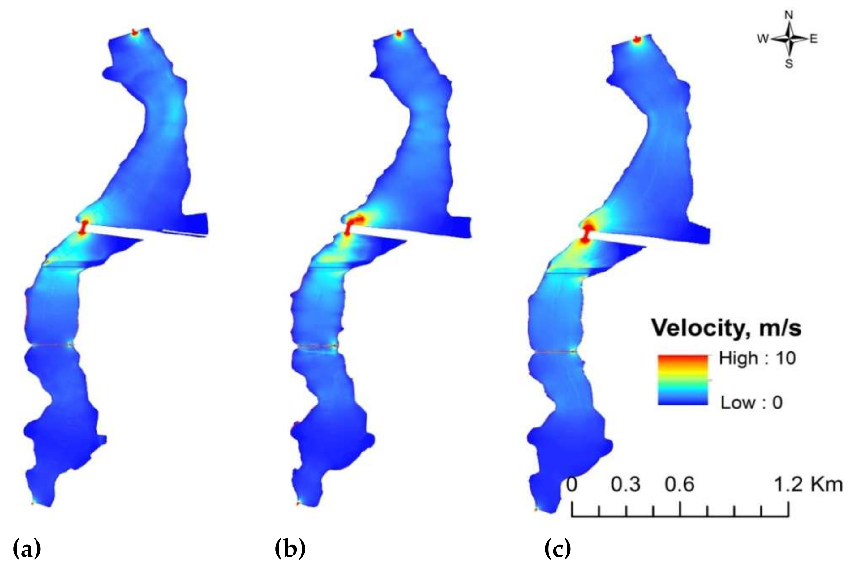
The graphs presented in Figure 11 illustrate the spatial distribution of maximum magnitudes of velocity in the reservoir. According to the maps, the maximum velocities occurred near structures such as the internal dam, the sluice in the internal dam, the flow below the bridge, and the reservoir outflow. There were also greater velocities in the reservoir inlet, though the area is so small that it was not visible well in the scale of Figure 11. The internal dam separates the preliminary part of the reservoir from its main part. The single and very small sluice caused local increase in the velocity magnitude and erosion of the alluvial bed. The maximum velocities over 3 m/s occurred also below the bridge. The reason was the too narrow bridge span.
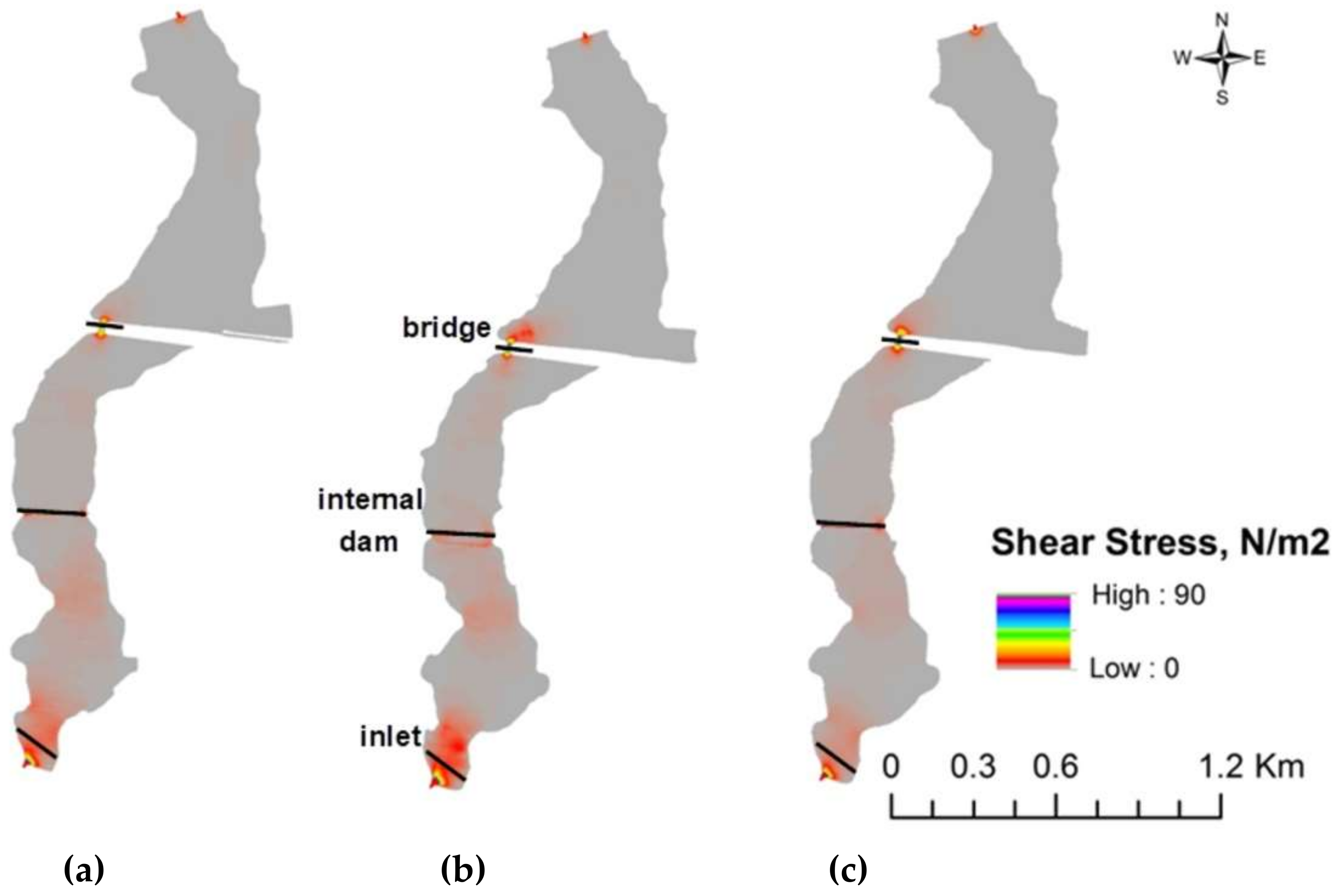
The results presented ealier were confirmed by the results shown in Figure 12a–c, illustrating that the distribution of the shear stresses in the reservoir was similar to that of velocity. The maximum values occurred at the reservoir inlet, near the internal dam, and in the bridge span. Additionally, the reservoir inlet was more prone to shear stress increase. The maximum shear stresses occurred for the bathymetry of 2013 (Figure 12b). In the bathymetry of 2018, the corresponding values were lower, especially, in the pre-reservoir. Supposedly, the artificial change in the bottom configuration as a result of dredging in 2014/2015 was the reason for such a change. Additionally, the very specific cross-sections marked in Figure 12 are cross-sections near the inlet, in the internal dam, and under the bridge. They were applied for analyses presented in Figure 13.
The next variable analyzed was the stream power [41,42,43], but it is shown only in the graphs created with one of two methods: (1) as cross-sections with results extracted from results in raster format (Figure 8a and Figure 12) (2) as statistics of values in the random sample points (Figure 8b). In Figure 13a–c, the graphs of shear stresses (SS) and stream power (SP) in selected cross-sections are shown for comparison. The cross-sections applied were those shown in Figure 12. In Figure 13a, the inlet cross-section is presented. The shear stresses (SS) simulated there were over 20 N/m2, while the stream power (SP) values reached about 100 W/m. The highest values of shear stress as well as stream power were observed for the reservoir in 2013. Supposedly, the accumulation of sediments in the period 2006–2013 changed the configuration of the bottom in such a way that there was an increase in these two factors. The values of shear stress and stream power were lower for the conditions in 2018. The removal of sediments in the pre-reservoir in 2014/2015 induced another kind of change. The next specific cross-section is shown in Figure 13b, at the internal dam with its sluice gate. The shear stresses as well as stream power in the sluice were increasing rapidly, independently of the bottom configuration tested. However, the sluice gate is made of concrete and it should be resistant to such forces. The huge values of the analyzed variable are more dangerous for the rest of the internal dam. The maximum values of shear stress were about 40 N/m2 there, while the stream power reached about 200 W/m. The values of these two factors were relatively small for the conditions in 2006, but in other configurations of the bottom, 2013 and 2018, high shear stresses and stream power were noticed. These values were quite high, especially in the lowland reservoirs where fine sand is deposited with grain sizes smaller than 0.5 mm. It means that, irrespective of the dredging and rebuild of the sluice gate, the internal dam is still exposed to huge forces and is prone to break. In the cross-section of the bridge, the shear stresses were smaller, about 7 N/m2 and seem to be stable. The same was noticed about the stream power values obtained there. The hydraulic conditions under the bridge seemed to be less dependent on the bottom configuration.
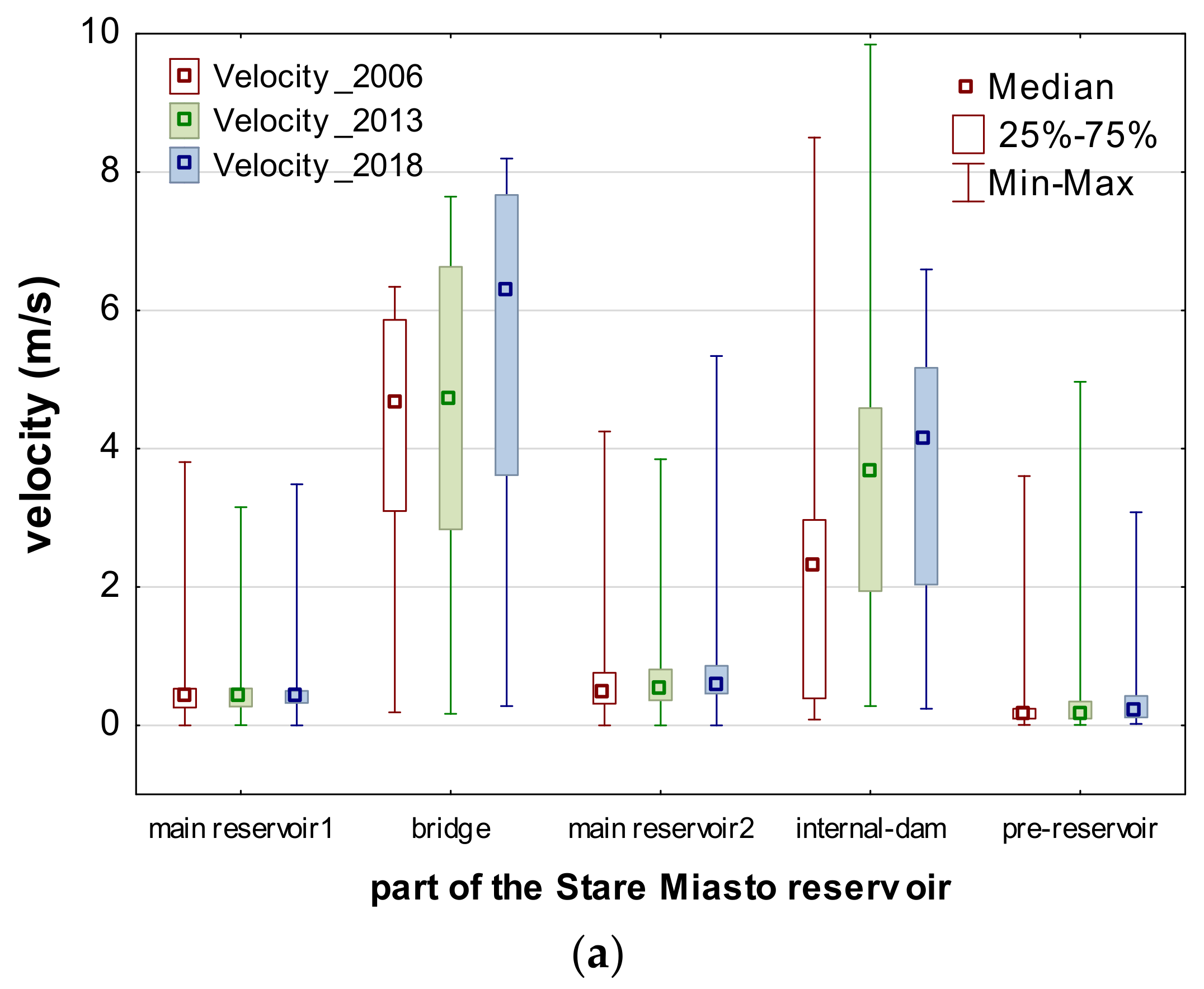
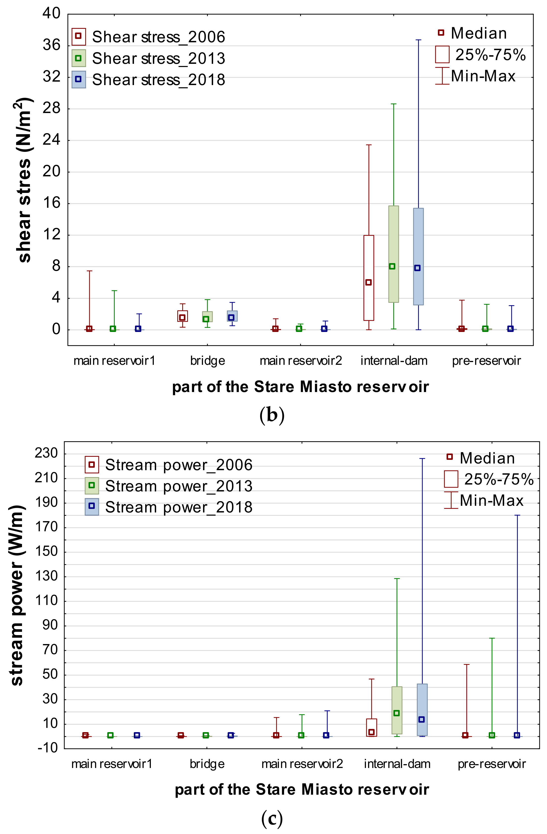
The next stage of the research was statistical analysis performed with Statistica 13. The values of maximum magnitudes of velocity, maximum shear stresses, and maximum stream power were read in the locations of the randomly generated points shown in Figure 8b, and then processed over the set of points and subsets included in particular reservoir parts (Figure 8a). Such results are presented as standard box-and-whisker plots in Figure 14a–c. The graph in Figure 14a shows the maximum flow velocities for different parts of the reservoir indicated in Figure 8a. The total medians were 0.32, 0.41, and 0.44 for bathymetries 2006, 2013, and 2018, respectively, while the mean values were 0.53, 0.67, 0.73 m/s. The significant differences between median and mean values for all bathymetries were caused by greater velocities calculated for the bridge and the internal dam. In the first case, the medians were 4.69, 4.81, and 6.38 m/s for the same bathymetries as previously. In the internal dam these factors reach values 2.33, 3.65, and 4.11 m/s. Such great irregularities indicate the importance of these two locations. The greatest values for all bathymetries were noticed under the bridge and over the internal dam. The velocities simulated with the initial bathymetry were slightly smaller than the others. The similarity of the internal dam median velocities for 2013 and 2018 shows that the dredging in 2014/2015 did not improve the safety of this dam much. Fortunately, the maximum velocities decreased from about 10 m/s in 2013 to 6–7 m/s in 2018. In the other parts of the reservoir, the velocities obtained were much smaller irrespective of the bathymetry tested.
The trends observed in the spatial distributions of shear stresses (Figure 14b) and stream power (Figure 14c) were different. Definitely the highest values of these two variables were observed in the internal dam. The discrepancy of the velocity magnitudes with shear stress and stream power observed under the bridge may be explained by relatively great narrowing of the flow area but small hydraulic slope governed by the head in the main dam. The internal dam influenced from the upstream and downstream was in different conditions. Hence, the shear stress and stream power confirm the observations of velocities.
It is also important that there is a difference in trend between the median and maximum values. The median values of the shear stress as well as stream power more or less decreased between 2013 and 2018. The simulation over the bottom for 2013 provided median shear stress equal to 7.95 N/m2 and median stream power of 27.97 W/m over the internal dam. The median results obtained for bathymetry 2018 were 7.77 N/m2 and 19.27 W/m, respectively. Hence, the decreases were 2.2% and 31.1% for shear stress and stream power, respectively. The same results indicate significant increases of the maximum values in the case of these two factors. The maximum shear stress and stream power values for bottom for 2013 were 28.63 N/m2 and 653.78 W/m, respectively. The results for the bathymetry 2018 gave maximum values of the same variables equaling 36.75 N/m2 and 815.12 W/m. Hence, the increase of shear stress was 28.4% and the increase of the stream power was 24.7%. It confirms the previous conclusion that the rebuild of the internal dam and sluice gate did not improve the safety of this object.
The analysis of bed changes and shear stress or stream power in reservoirs is relatively difficult for modeling. In many papers there is a description of the shear stresses acting on the river bed in mountainous as well as lowland conditions [30,44,45]. The majority of such concepts is based on the simulation in 1D or calculated with empirical formulae [30,45]. In results provided by Glock et al. [30], who simulated flow in Austrian rivers and a laboratory flume, shear stresses varied from 0.4 to 93 N/m2. The course of the channel, meandering or straight, influenced the obtained values greatly. The results were also dependent on the type of model applied. They compared results of 1D, 2D, and 3D models. It is obvious that shear stresses are impacted by the roughness of the channel bed and flow velocities. In the Stare Miasto reservoir maximum velocities up to 10 m/s (Figure 14a) generated huge shear stresses, reaching values of 90 N/m2 (Figure 13b). Such magnitudes were noted in the internal dam and near the sluice installed there. Huge velocities and shear stresses caused huge values of stream power. In the sluice it was 900 W/m (Figure 13b). During the flood wave propagation in the reservoir, the most critical location was the reservoir inlet. The velocities simulated there equaled 5 m/s (Figure 11), which was related to huge shear stresses reaching values of 25 N/m2 (Figure 13a).
5. Conclusions
The impact of hydraulic parameters, such as velocity, shear stress, and stream power, on the operational conditions in a two-stage reservoir was analyzed. The basis for the investigations was simulations assuming the 2D hydrodynamic model. Such an approach enabled better illustration of the processes and changes in the reservoir for different moments of time. The method applied was different from the 1D models usually applied, as it enabled better recognition of the advantages and drawbacks of two-stage constructions. The shear stresses were calculated for the entire reservoir basin and especially for the structures located in it, and visualization revealed significant differences in response to impacts such as flood wave propagation. The simulations were made for the bathymetries of 2006, 2013, and 2018. The conclusions drawn from the results indicated really great stresses exerted on the internal dam, which may lead to breakage of the dam structure. In general, the analyses proved that structures in the reservoir are prone to profound stresses. The magnitudes of shear stresses in specific flood conditions are not observed frequently in lowland rivers and reservoirs. The contraction caused by the bridge span is also very dangerous. In flooding conditions, it may cause great acceleration of water flow. The highway bridge is a massive construction and no direct threat related to great stress has been detected in this case. However, it is not possible to exclude the probability of erosion below the bridge and collapse of the construction due to bridge scour in future. One thing is obvious—the velocities, the shear stress, and stream power values are not typical of lowland conditions if the flood propagates through the reservoir. The presented analyses confirm that two-stage reservoirs are a good solution of some reservoir problems, if the inflows are moderate. However, the increase in inflows up to flood magnitudes may generate new problems related to the stability of the structures located in the reservoir basin.
The applied 2D hydrodynamic modeling enabled more detailed analysis focused on spatial distributions of important factors: the velocity, the shear stress, and the stream power. The obtained results are satisfactory and they may be applied in several ways. The approach presented enabled identification of potential threats, which is well shown on the example of the internal dam. However, such an approach required greater computational costs than in other cases—more simulation time, faster processors, more effective models, more memory on disks, etc. Although, the use of three different bathymetries and comparisons between them increased the complexity of the problem, it also enabled simplified verification of the object vulnerability to flood hazard. As indicated, the rebuild of the internal dam did not improve the safety of this structure and future breakage could be expected. Some application areas of the results presented seem to be obvious—improvement of reservoir design, optimization of structure shapes, invention of protective elements reducing detected threats. Others are not so obvious (e.g., operational control of reservoir to safely propagate the flood wave). However, such an approach requires greater computational power than that applied in this research.
As can be seen, the two-stage reservoirs are quite an interesting alternative approach to prevention of reservoir sedimentation. However, their construction should be carefully analyzed and computationally tested before the main dam is built. The results of the present research could help in the design of crucial elements, such as the sluice in the internal dam, the span of the bridge, etc. All such elements could cause unexpected effects dangerous for the stability of the reservoir construction and safety of the water management in the reservoir.
Author Contributions
Conceptualization; methodology; software; validation; formal analysis; investigation; resources; data curation; writing—original draft preparation; writing—review and editing; visualization; supervision; project administration; and funding acquisition, J.W.-D.
Funding
This research received no external funding.
Acknowledgments
This research would not be possible without the access to the data provided by such institutions as IMGW, CODGiK, and GUGiK. The access to the free data available in the Internet, such as Geoportal 2, was also very helpful.
Conflicts of Interest
The author declares no conflict of interest.
References
- RZGW. National Board for Water Management. Available online: https://warszawa.rzgw.gov.pl/the-regional-water-management-authority-in-warsaw 2018 (accessed on 5 March 2019).
- Schleiss, A.J.; Franca, M.J.; Juez, C.; De Cesare, G. Reservoir sedimentation. J. Hydraul. Res. 2016, 54, 595–614. [Google Scholar] [CrossRef]
- Dysarz, T.; Wicher-Dysarz, J.; Przedwojski, B. Man-induced morphological processes in Warta river and their impact on the evolution of hydrological conditions. In River Flow; Ferreira, R.M.L., Alves, E.C.T.L., Leal, J.G.A.B., Cardosa, A.H., Eds.; Taylor & Francis Groups: London, UK, 2006; pp. 1301–1310. [Google Scholar]
- Wicher-Dysarz, J.; Dysarz, T. Uncertainty in assessment of annual inflow of sediments to the Stare Miasto reservoir based on empirical formulae. Acta Sci. Pol. Form. Circumiectus 2015, 14, 201–212. [Google Scholar] [CrossRef]
- Sojka, M.; Jaskuła, J.; Wicher-Dysarz, J.; Dysarz, T. Poznań Univeristy of Life Sciences Analysis of Selected Reservoirs Functioning in the Wielkopolska Region. Acta Sci. Pol. Form. Circumiectus 2017, 4, 205–215. [Google Scholar] [CrossRef]
- Szoszkiewicz, K.; Wicher-Dysarz, J.; Sojka, M.; Dysarz, T. Assessment of hydraulic, hydrological and physicochemical factors affecting vegetation development in dam reservoir with separated inlet zone—Stare Miasto (central Poland) reservoir as a case study. Fresenius Environ. Bull. 2016, 25, 2772–2783. [Google Scholar]
- Ptak, M.; Sojka, M.; Choiński, A.; Nowak, B. Effect of environmental conditions and morphometric parameters on surface water temperature in Polish lakes. Water 2018, 10, 580. [Google Scholar] [CrossRef]
- Michalec, B. Appraisal of methods of determination of sediment quantity supplied to a small water reservoir. Arch. Environ. Prot. 2008, 34, 49–62. [Google Scholar]
- Michalec, B.; Tarnawski, M. The influence of small water reservoir operational changes on capacity reduction. Environ. Prot. Eng. 2008, 34, 117–124. [Google Scholar]
- Michalec, B. Evaluation of an empirical reservoir shape function to define sediment distributions in small reservoirs. Water 2015, 7, 4409–4426. [Google Scholar] [CrossRef]
- Dysarz, T.; Wicher-Dysarz, J. Analysis of flow conditions in the Stare Miasto Reservoir taking into account sediment settling properties. Annu. Set Environ. Prot. 2013, 15, 584–605. [Google Scholar]
- Dong, N.; Yang, M.; Meng, X.; Liu, X.; Wang, Z.; Wang, H.; Yang, C. CMADS-driven simulation and analysis of reservoir impacts on the streamflow with a simple statistical approach. Water 2019, 11, 178. [Google Scholar] [CrossRef]
- Jaskuła, J.; Sojka, M.; Wicher-Dysarz, J. Analysis of the vegetation process in a two-stage reservoir on the basis of satellite imagery—A case study: Radzyny Reservoir on the Sama River. Annu. Set Environ. Prot. 2018, 20, 203–220. [Google Scholar]
- Sojka, M.; Jaskuła, J.; Siepak, M. Heavy metals in bottom sediments of reservoirs in the lowland area of western Poland: Concentrations, distribution, sources and ecological risk. Water 2019, 11, 56. [Google Scholar] [CrossRef]
- Sojka, M.; Siepak, M.; Jaskuła, J.; Wicher-Dysarz, J. Heavy metal transport in a river-reservoir system: A case study from central Poland. Pol. J. Environ. Stud. 2018, 27, 1725–1734. [Google Scholar] [CrossRef]
- Sojka, M.; Jaskuła, J.; Wróżynski, R.; Waligórski, B. Application of sentinel-2 satellite imagery to assessment of spatio-temporal changes in the reservoir overgrowth process—A case study: Przebedowo, West Poland. Carpathian J. Earth Environ. Sci. 2019, 14, 39–50. [Google Scholar] [CrossRef]
- Sojka, M.; Siepak, M.; Gnojska, E. Assessment of heavy metal concentration in bottom sediments of Stare Miasto pre-dam reservoir on the Powa River. Annu. Set Environ. Prot. 2013, 15, 1916–1928. [Google Scholar]
- Wicher-Dysarz, J.; Kanclerz, J. Functioning of small lowland reservoirs with pre-dam zone on the example of Kowalskie and Stare Miasto Lakes. Rocznik Ochrona Srodowiska 2012, 14, 885–897. [Google Scholar]
- Kasperek, R.; Wiatkowski, M. Research on the Mściwojów reservoir. Sci. Rev. Eng. Environ. Sci. 2008, 40, 194–201. (In Polish) [Google Scholar]
- Paul, L. Nutrient elimination in pre-dams: Results of long term studies. Hydrobiologia 2003, 504, 289–295. [Google Scholar] [CrossRef]
- Pikul, K.; Mokwa, M. Influence of pre-dams on the main reservoir silting process. Sci. Rev. Eng. Environ. Sci. 2008, 17, 185–193. (In Polish) [Google Scholar]
- Paul, L.; Pütz, K. Suspended matter elimination in a pre-dam with discharge dependent storage level regulation. Limnol. Ecol. Manag. Inland Waters 2008, 38, 388–399. [Google Scholar] [CrossRef] [Green Version]
- Dysarz, T.; Wicher-Dysarz, J.; Sojka, M. Two approaches to forecasting of sedimentation in the Stare Miasto reservoir, Poland. In Reservoir Sedimentation; Taylor & Francis Group: London, UK, 2014; ISBN 978-1-138-02675-9. [Google Scholar]
- Krenkel, P.A.; Novotny, V. Water Quality Management; Academic Press: Cambridge, MA, USA, 1980. [Google Scholar]
- Szymkiewicz, R. Numerical Modeling in Open Channel Hydraulics; Springer: Berlin, Germany, 2010. [Google Scholar]
- Chow, V.T. Open-Channel Hydraulic; McGraw-Hill: New York, NY, USA, 1959. [Google Scholar]
- Wu, W. Computational River Dynamics; CRC Press: Boca Raton, FL, USA, 2007. [Google Scholar]
- Radecki-Pawlik, A.; Pagliara, S.; Hradecky, J. Basics of Open Channel Hydraulics, River Training and Fluvial Geomorphology; CRC Press: Boca Raton, FL, USA, 2016. [Google Scholar]
- Juárez, A.; Adeva-Bustos, A.; Alfredsen, K.; Dønnum, B.O. Performance of a two-dimensional hydraulic model for the evaluation of stranding areas and characterization of rapid fluctuations in hydropeaking rivers. Water 2019, 11, 201. [Google Scholar] [CrossRef]
- Glock, K.; Tritthart, M.; Habersack, H.; Hauer, C. Comparison of hydrodynamics simulated by 1D, 2D and 3D models focusing on bed shear stresses. Water 2019, 11, 226. [Google Scholar] [CrossRef]
- Marshal Office of the Wielkopolska Region in Poznan. Small Retention Program. Available online: https://umww.pl/o-programie-malej-retencji (accessed on 2018). (In Polish).
- Woliński, J.; Zgrabczyński, J. The Stare Miasto Reservoir in the Powa River: Water Management Rules; BIPROWODMEL Sp. z o.o.: Poznań, Poland, 2008. (In Polish) [Google Scholar]
- Preibisz, J.; Matan, J.; Woliński, J. Studium zabudowy retencyjnej rzeki Powy, Dokumentacja; BIPROWODMEL Sp. z o.o.: Poznań, Poland, 2000. (In Polish) [Google Scholar]
- IMGW. Public Data IMGW-PIB. Available online: https://dane.imgw.pl/ (accessed on 5 March 2019).
- Docan, D.C. Learning ArcGIS for Desktop; Packt Publishing: Birmingham, UK, 2016; Available online: https://www.packtpub.com/application-development/learning-arcgis-desktop (accessed on 7 July 2018).
- Cameron, T.; Ackerman, P.E. HEC-GeoRAS GIS Tools for Support of HEC-RAS using ArcGIS User’s Manual; US Army Corps of Engineers, Institute for Water Resources, Hydrologic Engineering Center (HEC): Davis, CA, USA, 2012; Available online: http://www.hec.usace.army.mil/software/hec-georas/documentation/HEC-GeoRAS_43_Users_Manual.pdf (accessed on 7 July 2018).
- Dysarz, T. Development of RiverBox—An ArcGIS toolbox for river bathymetry reconstruction. Water 2018, 10, 1266. [Google Scholar] [CrossRef]
- Brunner, G.W. HEC-RAS River Analysis System Hydraulic Reference Manual; US Army Corps of Engineers; Report No. CPD-69; Hydrologic Engineering Center (HEC): Davis, CA, USA, 2016. [Google Scholar]
- Brunner, G.W. HEC-RAS River Analysis System User’s Manual Version 5.0; US Army Corps of Engineers; Report No. CPD-68; Hydrologic Engineering Center (HEC): Davis, CA, USA, 2016. [Google Scholar]
- Van Rijn, L.C. Sediment transport. Part I: Bed load transport. J. Hydraul. Eng. 1984, 110, 1431–1456. [Google Scholar] [CrossRef]
- Bagnold, R. An Approach to the Sediment Transport Problem from General Physics; United States Government Printing Office: Washington, DC, USA, 1966.
- Yang, C.T. Unit stream power equation for gravel. J. Hydraul. Divis. 1984, 110, 1783–1797. [Google Scholar] [CrossRef]
- Yang, C.T. Sediment Transport: Theory and Practice; McGraw-Hill Companies, Inc.: New York, NY, USA, 1996. [Google Scholar]
- Radecki-Pawlik, A.; Kuboń, P.; Radecki-Pawlik, B.; Plesiński, K. Bed-load transport in two different-sized mountain catchments: Mlynne and Lososina streams, Polish Carpathians. Water 2019, 11, 272. [Google Scholar] [CrossRef]
- Radecki-Pawlik, A. Determination of nondimensionalization shear stress shields criterion used to calculate the initiationof motion of sediment using different formulae. Acta Sci. Pol. Form. Circumiectus 2015, 14, 75–107. (In Polish) [Google Scholar]
Figure 1.
Chosen case study—Stare Miasto reservoir on the Powa river: (a) The reservoir and its main elements—internal dam, highway bridge, and main dam; (b) the watershed with main elements—river, reservoirs, and gauge station.
Figure 1.
Chosen case study—Stare Miasto reservoir on the Powa river: (a) The reservoir and its main elements—internal dam, highway bridge, and main dam; (b) the watershed with main elements—river, reservoirs, and gauge station.

Figure 2.
Variability of discharge at the Posoka gauge station, (a) for the period 1971–2017; (b) for the year 2014.
Figure 2.
Variability of discharge at the Posoka gauge station, (a) for the period 1971–2017; (b) for the year 2014.

Figure 3.
Stare Miasto reservoir in the Powa river: (a) The internal dam in 2011; (b) the internal dam destroyed after the flood wave propagation in 2014; (c) the uncovered reservoir bottom near the internal dam (author: J. Wicher-Dysarz).
Figure 3.
Stare Miasto reservoir in the Powa river: (a) The internal dam in 2011; (b) the internal dam destroyed after the flood wave propagation in 2014; (c) the uncovered reservoir bottom near the internal dam (author: J. Wicher-Dysarz).

Figure 4.
Stare Miasto in the Powa river: (a) The bridge with highway A2; (b) the sluice in the internal dam in 2011; (c) the sluice in the internal dam in 2014 (author J. Wicher-Dysarz).
Figure 4.
Stare Miasto in the Powa river: (a) The bridge with highway A2; (b) the sluice in the internal dam in 2011; (c) the sluice in the internal dam in 2014 (author J. Wicher-Dysarz).

Figure 5.
Examples of data used for the reconstruction of the reservoir bathymetries: (a) Location of the selected area; (b) design map from 2006; (c) measurement points from 2013; (d) measurement points from 2018.
Figure 5.
Examples of data used for the reconstruction of the reservoir bathymetries: (a) Location of the selected area; (b) design map from 2006; (c) measurement points from 2013; (d) measurement points from 2018.

Figure 6.
Main ideas of the bathymetry reconstruction with RiverBox [37]: (a) Scheme of interpolation; (b) applied algorithm.
Figure 6.
Main ideas of the bathymetry reconstruction with RiverBox [37]: (a) Scheme of interpolation; (b) applied algorithm.

Figure 7.
Estimation of roughness coefficients: (a) Statistics of roughness coefficients calculated on the basis of approaches presented in Table 1; (b) sieve curves applied for the calculation of roughness coefficients.
Figure 7.
Estimation of roughness coefficients: (a) Statistics of roughness coefficients calculated on the basis of approaches presented in Table 1; (b) sieve curves applied for the calculation of roughness coefficients.

Figure 8.
Elements used in the analyses: (a) Parts of the reservoir and location of cross-sections; (b) location of sample points.
Figure 8.
Elements used in the analyses: (a) Parts of the reservoir and location of cross-sections; (b) location of sample points.

Figure 9.
Analysis of depth distributions over the reservoir bottom in the Stare Miasto reservoir: (a) Bathymetry 2006; (b) bathymetry 2013; (c) bathymetry 2018.
Figure 9.
Analysis of depth distributions over the reservoir bottom in the Stare Miasto reservoir: (a) Bathymetry 2006; (b) bathymetry 2013; (c) bathymetry 2018.

Figure 10.
Selected cross-sections: (a) Bottom and water surface elevations for three bathymetries; (b) difference in bottom elevations between 2006 and 2013, as well as between 2006 and 2018.
Figure 10.
Selected cross-sections: (a) Bottom and water surface elevations for three bathymetries; (b) difference in bottom elevations between 2006 and 2013, as well as between 2006 and 2018.

Figure 11.
Spatial distributions of velocities in the Stare Miasto reservoir for three bathymetries: (a) Bathymetry 2006; (b) bathymetry 2013; (c) bathymetry 2018.
Figure 11.
Spatial distributions of velocities in the Stare Miasto reservoir for three bathymetries: (a) Bathymetry 2006; (b) bathymetry 2013; (c) bathymetry 2018.

Figure 12.
Shear stress calculated for the Stare Miasto reservoir and three bathymetries: (a) Bathymetry 2006; (b) bathymetry 2013; (c) bathymetry 2018.
Figure 12.
Shear stress calculated for the Stare Miasto reservoir and three bathymetries: (a) Bathymetry 2006; (b) bathymetry 2013; (c) bathymetry 2018.

Figure 13.
Shear stress and stream power in chosen cross-section: (a) inlet; (b) internal dam; (c) bridge.
Figure 13.
Shear stress and stream power in chosen cross-section: (a) inlet; (b) internal dam; (c) bridge.

Figure 14.
Characteristic values of analyzed hydraulic parameters simulated for bathymetries 2006, 2013, and 2018, and recorded at random points: (a) Velocity; (b) shear stress; (c) stream power.
Figure 14.
Characteristic values of analyzed hydraulic parameters simulated for bathymetries 2006, 2013, and 2018, and recorded at random points: (a) Velocity; (b) shear stress; (c) stream power.


Table 1.
The dependence between absolute roughness and characteristics of sediment grain sizes.
| Methods | Absolute Roughness (ks) |
|---|---|
| Nikuradse | ks = 2.3d80 |
| Einstein | ks = d65 |
| Engelung-Hansen | ks = 2d65 |
| van Rijn | ks = 3d90 |
| Kamphuis | ks = 2d90 |
© 2019 by the author. Licensee MDPI, Basel, Switzerland. This article is an open access article distributed under the terms and conditions of the Creative Commons Attribution (CC BY) license (http://creativecommons.org/licenses/by/4.0/).
Share and Cite
MDPI and ACS Style
Wicher-Dysarz, J. Analysis of Shear Stress and Stream Power Spatial Distributions for Detection of Operational Problems in the Stare Miasto Reservoir. Water 2019, 11, 691. https://doi.org/10.3390/w11040691
AMA Style
Wicher-Dysarz J. Analysis of Shear Stress and Stream Power Spatial Distributions for Detection of Operational Problems in the Stare Miasto Reservoir. Water. 2019; 11(4):691. https://doi.org/10.3390/w11040691
Chicago/Turabian StyleWicher-Dysarz, Joanna. 2019. "Analysis of Shear Stress and Stream Power Spatial Distributions for Detection of Operational Problems in the Stare Miasto Reservoir" Water 11, no. 4: 691. https://doi.org/10.3390/w11040691
Note that from the first issue of 2016, this journal uses article numbers instead of page numbers. See further details here.