The Exact Groundwater Divide on Water Table between Two Rivers: A Fundamental Model Investigation


Ministry of Education Key Laboratory of Groundwater Circulation and Environmental Evolution, China University of Geosciences, Beijing 100083, China
*
Author to whom correspondence should be addressed.
Water 2019, 11(4), 685; https://doi.org/10.3390/w11040685
Submission received: 13 March 2019
/
Revised: 29 March 2019
/
Accepted: 1 April 2019
/
Published: 2 April 2019
(This article belongs to the Section Hydrology)
Abstract
:The groundwater divide within a plane has long been delineated as a water table ridge composed of the local top points of a water table. This definition has not been examined well for river basins. We developed a fundamental model of a two-dimensional unsaturated–saturated flow in a profile between two rivers. The exact groundwater divide can be identified from the boundary between two local flow systems and compared with the top of a water table. It is closer to the river of a higher water level than the top of a water table. The catchment area would be overestimated (up to ~50%) for a high river and underestimated (up to ~15%) for a low river by using the top of the water table. Furthermore, a pass-through flow from one river to another would be developed below two local flow systems when the groundwater divide is significantly close to a high river.
1. Introduction
Hydrologists study the water cycle and transport of accompanying materials in regions based on watershed divisions. A watershed or drainage basin is an area enclosed by a divide line that can be described with topographic ridges, i.e., with local land surface top points. This definition is fine for surface water studies but is not always effective in groundwater studies. The groundwater divide between basins may be different from the topographic divide [1,2], and it causes inter-basin groundwater flow (IGF) that has been identified in hydrogeological surveys [2,3,4]. In the past few decades, researchers have highlighted the impacts of IGF on the geochemical characteristics [5,6,7], the regional climate–hydrological interactions [8], and the geomorphic evolution [9] of river basins. An exact description of groundwater divides is necessary to quantitatively interpret the features of IGF.
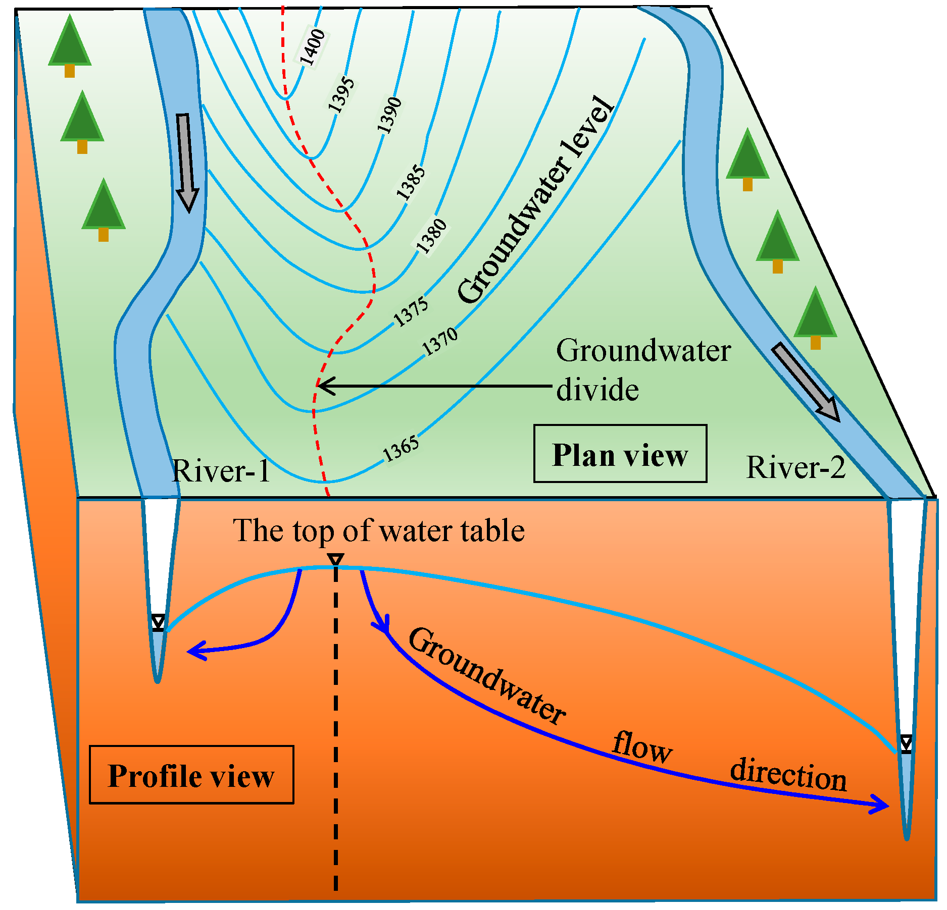
The definition of the groundwater divide is not as straightforward as it is for surface watersheds due to the complexities in aquifer media (geological and hydraulic diversity) and flow patterns (horizontal and vertical). At the regional scale, nested groundwater flow systems can develop [10,11], in which the flow system boundaries yield divide lines of groundwater on the profile and show how IGF occurs. In particular, water table highs linking with divide lines between local flow systems are comparable to surface watersheds [2]. In the horizontal plane, a groundwater divide has been conventionally defined as a curve representing the water table ridge (described with contours of the groundwater level) that separates the flow domain into subdomains [1]. For an unconfined aquifer with infiltration recharge between two rivers (Figure 1), in practice, people describe the groundwater divide as a line across the contours of the groundwater level at the turning points (in the plan view) that play a role as local top points of the water table (in the profile view). The point with the highest elevation on the water table between rivers is the theoretical place of groundwater divide, as in the Dupuit–Forchheimer model [12], where the vertical line below the point (dashed line in Figure 1) yields a no flow boundary. The Dupuit assumption ignores the vertical flow but this definition of groundwater divide is compatible with Tóth’s theory if only two local flow systems exist between the rivers. In most of the profile figures of nested flow systems [2,10,11,13,14], it is believed that water table highs separate the local flow systems. However, the relationship between the exact groundwater divide and the top of the water table in an inter-river unconfined aquifer, to our knowledge, has never been seriously examined in the literature.
The inaccuracy of using the water table ridge in defining the groundwater divide was recently noticed in an investigation of three-dimensional (3D) groundwater flow systems [15]. Groundwater circulation cells (GWCCs) have been defined as representing the unit space of groundwater flow from a recharge area to a discharge area. Local flow systems are characterized by open GWCCs with boundaries on the phreatic surface that are close to the local top of the water table. However, they do not coincide with and are not parallel to the water table ridges. The investigation was based on complex Tóthian basins where the flow patterns are controlled by an undulating water table which has a planar distribution of discharge zones. The water table plays a role as a subdued replica of the topography in these topography-controlled basins where the recharge is relatively high over the hydraulic conductivity of the aquifers [16]. In reality, for basins the flow systems are mostly controlled by areal recharge and linear discharge or local discharge at limited water table outcrops [17,18,19], especially for river basins. How is the groundwater divide different from the local top of the water table in a river basin? This question has not been well addressed. As an early investigation, we carried out a special examination of the groundwater divide between rivers in a fundamental two-dimensional (2D) profile model for an unconfined aquifer. Inconsistency between the exact groundwater divide and the top of the water table was found and quantitatively researched. We are aware that this is an essential effect for river basins with high ratios of groundwater discharge to streamflow.
2. Conceptual Model and Methods
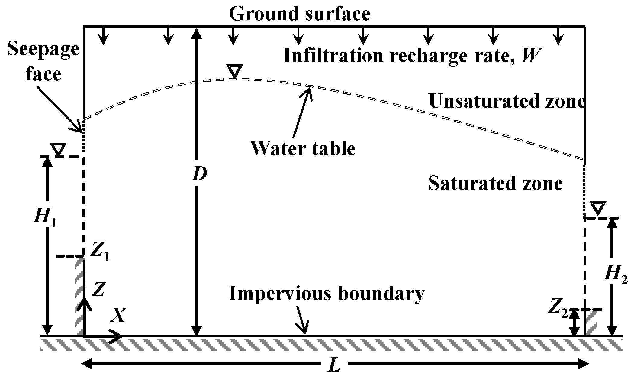
In this study, we analyzed the groundwater divide between rivers using a fundamental 2D model, as shown in Figure 2. The two rivers, numbered 1 and 2, partially cut into an unconfined aquifer with anisotropic homogeneous porous media. The water level in River 1 was higher than that in River 2. Precipitation infiltration proceeded at a constant uniform rate and drove a steady-state unsaturated–saturated flow from the ground surface to the rivers across the aquifer. A water table mound was formed, separating the saturated and unsaturated zones. Seepage faces were also formed along the interface between the aquifer and atmosphere when groundwater flowed to a surface body [1,12].
Assuming Darcy’s law was applicable, we adopted the Richards’ equation to describe the unsaturated–saturated flow in porous media [20]. The pressure head (L) of capillary water in the unsaturated zone, Ph, was used in the equation, which can be incorporated into the total hydraulic head (L), H, as [1]
where Z is the height (L) of the position (positive upward). Ph < 0 for positions in the unsaturated zone whereas Ph ≥ 0 in the saturated zone. At the position of the water table, Ph = 0. For the 2D steady-state flow in the model shown in Figure 2, the control equation can be written as
where Ksx and Ksz are the saturated hydraulic conductivities (LT−1) in the horizontal and vertical flow, respectively. Kr is the ratio (-) of hydraulic conductivities between unsaturated and saturated flow, and is a function of Ph. X is the horizontal distance (L) from the side of River 1. Without loss of generality, we used the exponential formula for Kr when Ph < 0, Kr = exp(AkPh) [21], where Ak (L−1) is a decay parameter; otherwise, Kr = 1. The empirical range of Ak for soils is 0.2–5.0 m−1 [22].
The boundary conditions were specified as
where W is the net infiltration rate (LT−1), D is the total thickness of the aquifer (L), and L is the horizontal length of the aquifer between the two rivers (L). H1 and H2 are the water levels in River 1 and River 2 (L), respectively. Z1 and Z2 are the river bed heights of River 1 and River 2 (L), respectively. Cb is a parameter (LT−1) dependent on the existence of a seepage face. Equation (8) is a simplified formula of the equation in Chui and Freyberg (2009) [23] used to switch the boundary condition between the Neumann type (Cb = 0 when H ≤ Z) for a place above the seepage face and the Dirichlet type (Cb→∞ when H > Z) for a portion at the seepage face. In practice, a large number is applied to estimate Cb→∞.
The mathematic model presented in Equations (2)–(8) can be solved in a general way with the dimensionless variables
where i = 1 and 2 denotes River 1 and River 2, respectively. Equation (2) can then be rewritten as
The boundary conditions can also be simplified with these dimensionless variables:
There are difficulties in obtaining the general analytical solution of Equation (12) because it is a nonlinear second-order partial differential equation. Read and Broadbridge [24] developed series solutions only for the case of ph < 0 so that the flow in the saturated zone was not incorporated. Tristscher et al. [25] extended the solutions to a condition with both unsaturated and saturated zones but an additional numerical approach has to be used. This analytical-numerical approach is not efficient for segmental boundaries such as that expressed in Equations (15)–(19). In this study, a numerical solution of the model was implemented using the COMSOL Multiphysics tool produced by COMSOL Inc., Sweden [26]. The maximum element size of the finite-element network was limited to 0.02. The water table was identified as the curve satisfying ph = 0. In particular, this software yielded a streamline tracing technique used to identify local flow systems (different groups of streamlines) for groundwater discharge toward River 1 and River 2. The boundary between the local flow systems intersected the water table at a point that performs a role as the exact divide but may be different from the top of the water table.
3. Results
The modeling results in the dimensionless manner are dependent on the geometric parameters, zi and hi, that are limited between 0 and 1, and the physical parameters, a, k, and w, that are defined in Equation (11). In this study, we set the a value to the range between 2 and 300 for D varying from 10 m to 60 m and Ak varying from 0.2 m−1 to 5.0 m−1 [22]. The k value varies between 0.1 and 10 for normal conditions where D is significantly smaller than L but Ksx is significantly higher than Ksz. The w value is less than 1 because W is generally smaller than Ksz. The parameter c is not a control parameter because it is 0 or ∞. A large enough number is used to estimate c→∞.
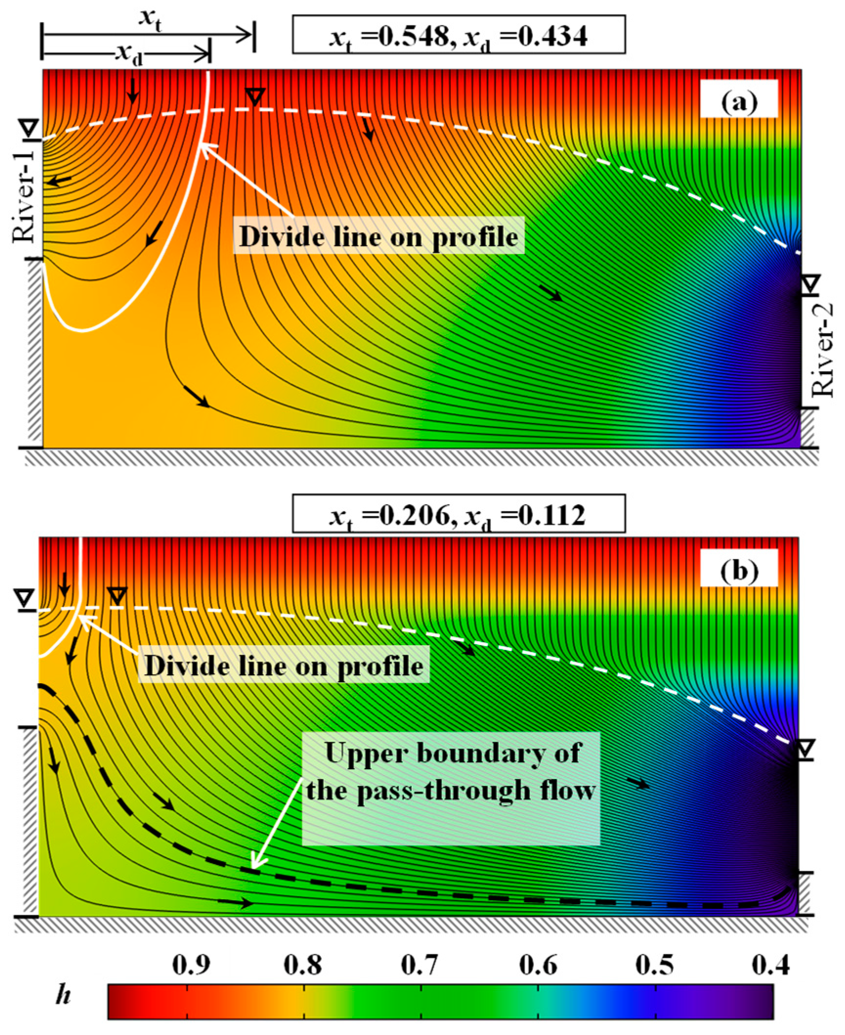
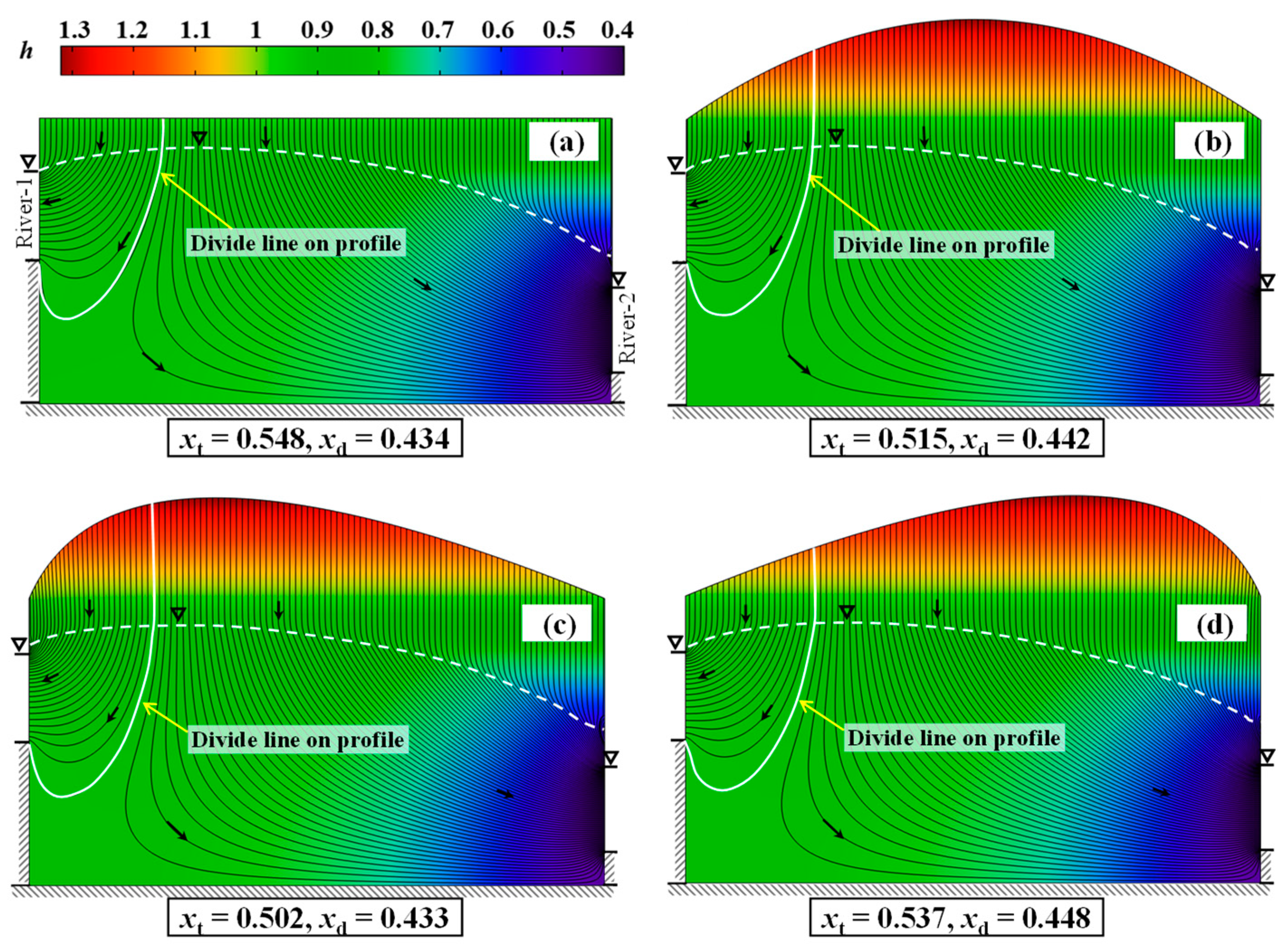
We show two typical cases in Figure 3 to indicate what will happen. In these cases, the water level in River 1 is double of that in River 2 so more infiltration recharge is contributed to River 2. Streamlines indicate the characteristics of the flow systems. A divide line exists between the local flow systems of the two rivers. The point of intersection between the divide line and the water table is not the top of the water table but closer to River 1. In the domain between the two points, a downward flow of shallow groundwater is accompanied by a weak horizontal flow toward River 1. However, in the deep zone, the flow changes direction in the horizontal direction toward River 2. This dynamic feature explains why the divide has to shift to a place that is closer to River 1. The relative errors can be calculated as
where xd and xt are dimensionless horizontal coordinates of the groundwater divide and the top of the water table, respectively. The errors in the catchment area estimated for River 1 and River 2 by using the top of water table, are, respectively, e1 and e2. The value of e1 in percentage denotes the overestimated proportion (e1 ≥ 0) of the catchment area for the high river. The negative value of e2 denotes underestimated proportion (e2 ≤ 0) of the catchment area for the low river. For the situations in Figure 3, the e1 values are +20.8% in Figure 3a and +45.6% in Figure 3b, respectively, showing a significant overestimation of the catchment area for River 1. The maximum e1 value in other examples approximates to 50%. In comparison, the e2 values are −7.9% for Figure 3a and −5.2% for Figure 3b, respectively. Thus, the catchment area was underestimated for River 2 but the absolute relative error was smaller than that for River 1.
A special feature was exhibited when the infiltration recharge was small, as shown in Figure 3b: a pass-through flow from River 1 to River 2 came into being below the local flow systems. This should not be the regional groundwater flow system or intermediate flow system that is defined in Tóth’s theory because the source head (River 1) of such a pass-through flow is a local discharge zone. When w is less than 0.06 without changes in other parameters, the divide of shallow groundwater disappears (xd = 0) and only a local flow system of River 2 overlies the pass-through flow. Thus, Figure 3b shows a transition status of groundwater flow between that shown in Figure 3a and that of w < 0.06.
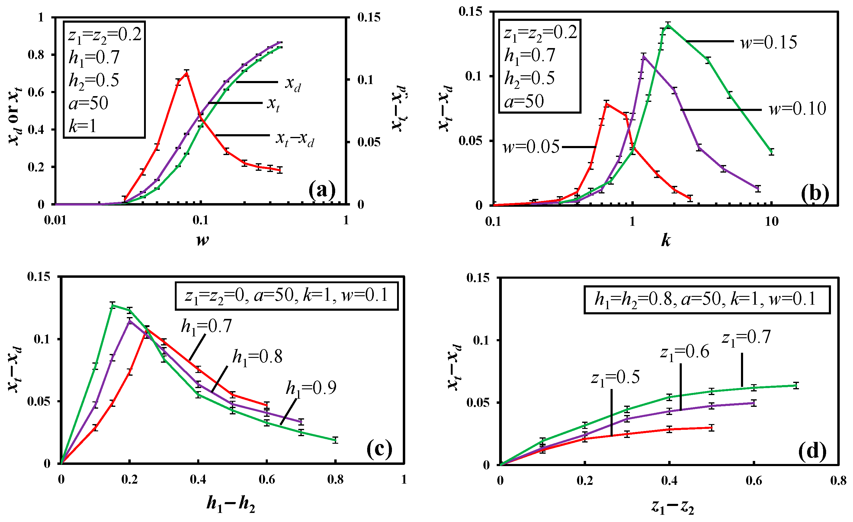
We checked the variation of the gap xt−xd with sensitivity analysis, as illustrated in Figure 4. Figure 4a shows the impact of the infiltration recharge w. In this case, there are four types of status of the flow. (1) The top of the water table lies on the side of River 1 (xt = xd = 0) when w < 0.03. (2) Two local flow systems overlie a pass-through flow when w ranges from 0.03 to 0.08. (3) The pass-through flow does not exist when w ranges from 0.08 to 0.35. (4) The top of the water table touches the ground surface when w > 0.35, leading to an overland flow. When w increases from 0.03 to 0.35, both xt and xd increase (the divide moves toward River 2) but xt−xd is raised to its maximum value when w = 0.08, after which point it decreases. Figure 4b shows similar rise–fall curves of xt−xd when k increases from 0.1 to 10.0. The peak value of xt−xd is raised with increasing w. A higher k value results in a divide closer to River 1 and increases the possibility of pass-through flow. Figure 4c explains the impact of the water level difference, h1−h2, for rivers that fully penetrate the aquifers (z1 = z2 =0). Increasing h1−h2 may push the divide toward River 1, whereas xt−xd varies along a rise–fall curve. The maximum xt−xd value is positively related to the water level in River 1. An equal water level does not mean the groundwater divide would lie on the top of the water table in the middle. As pointed out in Figure 4d, the difference in the penetrating depth of the rivers, z1−z2, is also a cause of the difference between xt and xd. Parameter a mainly controls the unsaturated flow and does not significantly influence the modeling results of the water table and streamlines.
The xt−xd values shown in Figure 4 are less than 0.15, showing that the e2 value determined from Equation (12) is higher than −15% (because xt is smaller than 1). Therefore, the underestimation of the catchment area for River 2 would be generally less than 15% by using the top of water table.
4. Discussion
The fundamental 2D model used in this study demonstrates how far a groundwater divide between two rivers would be removed from the top of the water table. The modeling results in a dimensionless manner which can be used directly to assess the actual difference between groundwater divides and water table highs if the conditions between rivers or drains are sufficiently similar to the model. However, this model includes assumptions and simplifications which should be carefully examined in practice.
4.1. The Effect of Using the Van Genuchten (1980) (VG) Formula for Kr
For the numerical modeling of flow in the unsaturated zone, the model used here may be enhanced by using more complex formulas of Kr that have been suggested by other researchers [27,28]. However, this would introduce a cost associated with using more empirical parameters. In this section, we examine the use of the VG formula for calculating Kr [27], the VG formula being
where
and α is a parameter (L−1) used for describing the soil retention curve, αD (=αD) is a dimensionless parameter which was introduced in this research, and n and l are dimensionless parameters. The value of l has been suggested as being 0.5 [27]. Thus, αD and n are the two dimensionless parameters considered in this study as being capable of rerunning the fundamental model on the basis of the VG formula. According to the database of soils proposed by Carsel and Parrish [29], the ranges of α and n are 0.2–14.5 m−1 and 1.09–2.68, respectively. The value of αD should range from 2 to 300 for normal conditions where D ranges from 10 m to 60 m.
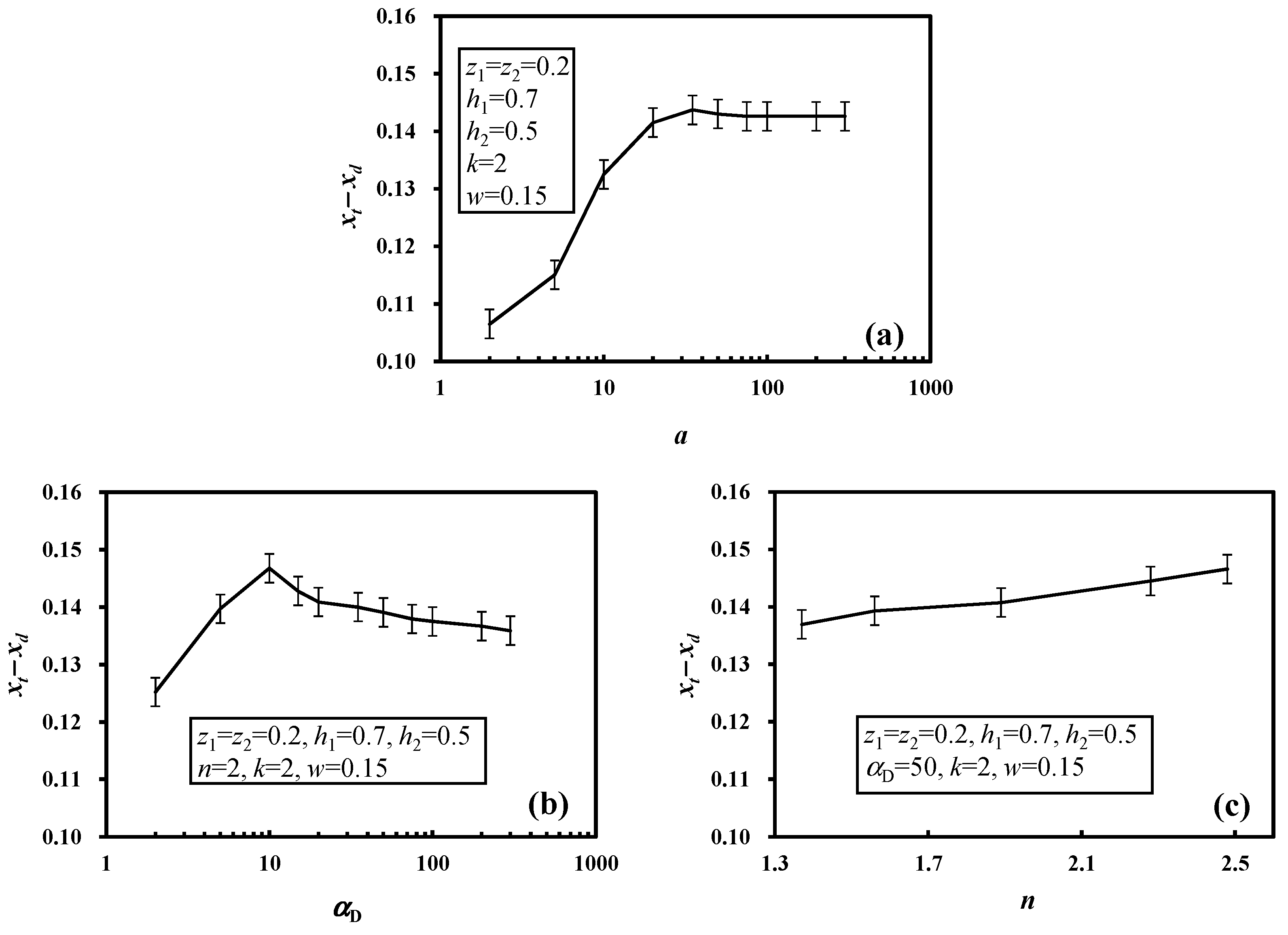
Typical results obtained using the Gardner formula (with only one dimensionless parameter, a) and VG the formula are presented for comparison in Figure 5. The values of xt−xd show different sensitivities with variations in a, αD, and n. As indicated in Figure 5a, the value of xt−xd generally increases with a when the value of a is less than 30, and then stays at an approximately constant value when the value of a is larger than 30. When the VG formula is used, as shown in Figure 5b, the relationship between xt−xd and αD is not consistent, and a peak value of xt−xd exists when αD is close to 10. It should be noted that both a and αD control the decay of hydraulic conductivity with decreases in soil water saturation and thus the impact of αD on xt−xd is comparable to the impact of a on xt−xd. Figure 5b shows a smaller variation range of xt−xd than that shown in Figure 5a. However, the maximum values of xt−xd obtained with the two Kr formulas are almost the same, being between 0.14 and 0.15. Compared to the results obtained using the Gardner formula, using the VG formula does not cause a significant underestimation of the maximum difference between the top of the water table and the groundwater divide. In addition, the xt−xd value is not significantly influenced by the n value, even though it increases with increasing n, as shown in Figure 5c. The e1 and e2 values estimated from the VG formulas were shown to be generally lower than 36% and higher than −10%, respectively. Therefore, it may be concluded that the use of the VG formula will not break the previously obtained boundary of relative difference between the top of the water table and the groundwater divide.
4.2. Examining the Effect of Topography
One of the assumptions of the fundamental model that should be examined is that regarding the flat horizontal ground surface. In mountain areas, two neighboring streams are generally separated by a hill, causing a surface water divide between them. We preliminarily checked the impact of such topography by reshaping the ground surface boundary in the model with a hill in the middle or on the left (closer to River 1) or right (closer to River 2). The boundary condition on the top may be rewritten from Equation (13) in this situation as
where f(x) is a function used here to describe the shape of the hill. The other boundary conditions are not changed.
Figure 6 shows examples where the hydraulic conditions and parameters coincide with those of Figure 3a, except for the shape of the ground surface. The shape of the water table does not significantly change because the infiltration recharge is the same. A hill in the middle increases xd but decreases xt, as shown in Figure 6b, resulting in a smaller gap (xt−xd) in comparison to that of a flat ground surface. When the hill is closer to River 1, as shown in Figure 6c, both xd and xt decrease but xt decreases more. When the hill is closer to River 2, as shown in Figure 6d, xd increases and xt decreases but xd increases more. Therefore, the gap between the groundwater divide and the top of the water table seems to be smaller than that seen in the fundamental model when a hill exists between the rivers, regardless of whether the hill is in the middle or not. However, further research should examine this effect using more examples.
5. Conclusions
The groundwater divide has been traditionally delineated as the line of local top points on the water table, which is similar to the definition of the surface water divide where topographic ridges are used. In this work, we examined this approach for river basins by using a fundamental 2D model of unsaturated–saturated flow in an unconfined aquifer between two rivers. The boundary between two local flow systems of the two rivers was identified, and it was shown to intersect the water table at the exact groundwater divide. In comparison with the top of the water table, the groundwater divide is closer to the river of the higher water level. The gap between them depends nonlinearly on the shape, size, boundary conditions, and hydraulic properties of the aquifer. The catchment area of the high river may be overestimated from the top of the water table with an error of up to ~50%. The catchment area of the low river may be underestimated but the error is generally less than 15%. A pass-through flow from one river to another will also develop below two local flow systems when the groundwater divide is significantly close to the high river. This is a new type of IGF—in comparison to regional groundwater flow—from which the rivers directly exchange water even when a divide has developed between them.
Author Contributions
P.-F.H. has contributed to run the model and write the paper. X.-S.W. has contributed to develop the conceptual and mathematical models. L.W., X.-W.J. and F.-S.H. have contributed to modify the computation process and discussions.
Funding
This study is supported by the National Natural Science Foundation of China (Grant no. 41772249) and the Fundamental Research Funds for the Central Universities (2652017169).
Conflicts of Interest
The authors declare no conflicts of interest.
References
- Bear, J. Hydraulics of Groundwater; McGraw-Hill: New York, NY, USA, 1979; pp. 55–59. [Google Scholar]
- Winter, T.C.; Rosenberry, D.O.; Labaugh, J.W. Where does the ground water in small watersheds come from? Ground Water 2003, 41, 989–1000. [Google Scholar] [CrossRef]
- Eakin, T.E. A regional interbasin groundwater system in the White River area, southeastern Nevada. Water Resour. Res. 1966, 2, 251–271. [Google Scholar] [CrossRef]
- Winograd, I.J. Interbasin groundwater flow in South Central Nevada: A further comment on the discussion between Davisson et al. (1999a, 1999b) and Thomas (1999). Water Resour Res. 2001, 37, 431–433. [Google Scholar] [CrossRef]
- Genereux, D.P.; Wood, S.J.; Pringle, C.M. Chemical tracing of interbasin groundwater transfer in the lowland rainforest of Costa Rica. J. Hydrol. 2002, 258, 163–178. [Google Scholar] [CrossRef]
- Genereux, D.P.; Jordan, M. Interbasin groundwater flow and groundwater interaction with surface water in a lowland rainforest, Costa Rica: A review. J. Hydrol. 2006, 320, 385–399. [Google Scholar] [CrossRef]
- Genereux, D.P.; Nagy, L.A.; Osburn, C.L.; Oberbauer, S.F. A connection to deep groundwater alters ecosystem carbon fluxes and budgets: Example from a Costa Rican rainforest. Geophys. Res. Lett. 2013, 40, 2066–2070. [Google Scholar] [CrossRef]
- Schaller, M.F.; Fan, Y. River basins as groundwater exporters and importers: implications for water cycle and climate modeling. J. Geophys. Res. Atmos. 2009, 114, 1–21. [Google Scholar] [CrossRef]
- Frisbee, M.D.; Tysor, E.H.; Stewart-Maddox, N.S.; Tsinnajinnie, L.M.; Wilson, J.L.; Granger, D.E.; Newman, B.D. Is there a geomorphic expression of interbasin groundwater flow in watersheds? Interactions between interbasin groundwater flow, springs, streams, and geomorphology. Geophys. Res. Lett. 2016, 43, 1158–1165. [Google Scholar] [CrossRef]
- Tóth, J. A theoretical analysis of groundwater flow in small drainage basins. J. Geophys. Res. 1963, 68, 4795–4812. [Google Scholar] [CrossRef]
- Tóth, J. Gravitational Systems of Groundwater Flow; Cambridge University Press: Cambridge, UK, 2009; pp. 62–65. [Google Scholar]
- Bear, J. Dynamics of Fluids in Porous Media; Dover Publications: New York, NY, USA, 1972; pp. 33–36. [Google Scholar]
- Tóth, J. Gravity-induced cross-formational flow of formation fluids, red earth region, alberta, Canada: Analysis, patterns, and evolution. Water Resour. Res. 1978, 14, 805–843. [Google Scholar] [CrossRef]
- Engelen, G.B.; Kloosterman, F.H. Numerical Modelling of Groundwater Flow Systems; a Case Study in the SE part of the Netherlands. Hydrological Systems Analysis; Springer: Delft, The Netherlands, 1996. [Google Scholar]
- Wang, X.S.; Wan, L.; Jiang, X.W.; Li, H.; Zhou, Y.; Wang, J.; Ji, X. Identifying three-dimensional nested groundwater flow systems in a Tóthian basin. Adv. Water Resour. 2017, 108, 139–156. [Google Scholar] [CrossRef]
- Haitjema, H.M.; Mitchellbruker, S. Are water tables a subdued replica of the topography? Ground Water 2005, 43, 781–786. [Google Scholar] [CrossRef]
- Liang, X.; Liu, Y.; Jin, M.; Lu, X.; Zhang, R. Direct observation of complex tóthian groundwater flow systems in the laboratory. Hydrol. Process. 2010, 24, 3568–3573. [Google Scholar] [CrossRef]
- Liang, X.; Quan, D.; Jin, M.; Liu, Y.; Zhang, R. Numerical simulation of groundwater flow patterns using flux as upper boundary. Hydrol. Process. 2013, 27, 3475–3483. [Google Scholar] [CrossRef]
- Bresciani, E.; Goderniaux, P.; Batelaan, O. Hydrogeological controls of water table -land surface interactions. Geophys. Res. Lett. 2016, 43, 9653–9661. [Google Scholar] [CrossRef]
- Richards, L.A. Capillary conduction of liquids through porous mediums. Physics 1931, 1, 318–333. [Google Scholar] [CrossRef]
- Gardner, W.R. Some steady-state solutions of the unsaturated moisture flow equation with application to evaporation from a water table. Soil Sci. 1958, 85, 228–232. [Google Scholar] [CrossRef]
- Philip, J.R. Theory of infiltration. Adv. Hydrosci. 1969, 5, 215–296. [Google Scholar]
- Chui, T.F.M.; Freyberg, D.L. Implementing hydrologic boundary conditions in a multiphysics model. J. Hydrol. Eng. 2009, 14, 1374–1377. [Google Scholar] [CrossRef]
- Read, W.; Broadbridge, P. Series solutions for steady unsaturated flow in irregular porous domains. Transp. Porous Media 1996, 22, 195–214. [Google Scholar] [CrossRef]
- Tristscher, P.; Read, W.W.; Broadbridge, P.; Knight, J.H. Steady saturated-unsaturated flow in irregular porous domains. Math. Comput. Modell. 2001, 34, 177–194. [Google Scholar] [CrossRef]
- COMSOL AB. COMSOL Multiphysics User’s Guide; COMSOL AB: Stockholm, Sweden, 2008. [Google Scholar]
- van Genuchten, M.T. A closed-form equation for predicting the hydraulic conductivity of unsaturated soils. Soil Sci. Soc. Am. J. 1980, 44, 892–898. [Google Scholar] [CrossRef]
- Brooks, R.H. Properties of porous media affecting fluid flow. J. Irrig. Drain. 1964, 92, 61–88. [Google Scholar]
- Carsel, R.F.; Parrish, R.S. Developing joint probability distributions of soil water retention characteristics. Water Resour. Res. 1988, 24, 755–769. [Google Scholar] [CrossRef]
Figure 1.
A schematic map of groundwater divide between two rivers according to traditional definition.
Figure 1.
A schematic map of groundwater divide between two rivers according to traditional definition.

Figure 2.
The conceptual model. H1 and H2 are the water levels in rivers where H1 ≥ H2.

Figure 3.
Streamlines (black curve) and hydraulic head distribution (color) in a case of z1 = 0.5, h1 = 0.8, z2 = 0.1, h2 = 0.4, k = 1, a = 50 with different infiltration conditions: (a) w = 0.22; (b) w = 0.12. Water table is shown as the dashed white line. Short arrows denote the flow direction.
Figure 3.
Streamlines (black curve) and hydraulic head distribution (color) in a case of z1 = 0.5, h1 = 0.8, z2 = 0.1, h2 = 0.4, k = 1, a = 50 with different infiltration conditions: (a) w = 0.22; (b) w = 0.12. Water table is shown as the dashed white line. Short arrows denote the flow direction.

Figure 4.
Dependency of the difference between xd and xt on control parameters. (a) w, (b) k, (c) h1–h2, (d) z1–z2.
Figure 4.
Dependency of the difference between xd and xt on control parameters. (a) w, (b) k, (c) h1–h2, (d) z1–z2.

Figure 5.
Dependency of the difference between xd and xt on control parameters in the Gardner formula, (a), and VG formula, (b) and (c).
Figure 5.
Dependency of the difference between xd and xt on control parameters in the Gardner formula, (a), and VG formula, (b) and (c).

Figure 6.
Change in the flow when the flat ground surface (a) is replaced by a hill with a peak in the middle (b) or in a place near River 1 (c) or River 2 (d). The same result in (a) has been shown in Figure 3a.
Figure 6.
Change in the flow when the flat ground surface (a) is replaced by a hill with a peak in the middle (b) or in a place near River 1 (c) or River 2 (d). The same result in (a) has been shown in Figure 3a.

© 2019 by the authors. Licensee MDPI, Basel, Switzerland. This article is an open access article distributed under the terms and conditions of the Creative Commons Attribution (CC BY) license (http://creativecommons.org/licenses/by/4.0/).
Share and Cite
MDPI and ACS Style
Han, P.-F.; Wang, X.-S.; Wan, L.; Jiang, X.-W.; Hu, F.-S. The Exact Groundwater Divide on Water Table between Two Rivers: A Fundamental Model Investigation. Water 2019, 11, 685. https://doi.org/10.3390/w11040685
AMA Style
Han P-F, Wang X-S, Wan L, Jiang X-W, Hu F-S. The Exact Groundwater Divide on Water Table between Two Rivers: A Fundamental Model Investigation. Water. 2019; 11(4):685. https://doi.org/10.3390/w11040685
Chicago/Turabian StyleHan, Peng-Fei, Xu-Sheng Wang, Li Wan, Xiao-Wei Jiang, and Fu-Sheng Hu. 2019. "The Exact Groundwater Divide on Water Table between Two Rivers: A Fundamental Model Investigation" Water 11, no. 4: 685. https://doi.org/10.3390/w11040685
Note that from the first issue of 2016, this journal uses article numbers instead of page numbers. See further details here.