Effect of Pilot-Points Location on Model Calibration: Application to the Northern Karst Aquifer of Qatar


1
Qatar Environment and Energy Research Institute (QEERI), Hamad Bin Khalifa University (HBKU), Doha P.O. Box 5825, Qatar
2
College of Science and Engineering, Hamad Bin Khalifa University (HBKU), Doha P.O. Box 5825, Qatar
3
Laboratoire d’Hydrologie et Géochimie de Strasbourg, University of Strasbourg/EOST/ENGEES, CNRS, 1 rue Blessig, 67084 Strasbourg, France
*
Author to whom correspondence should be addressed.
Water 2019, 11(4), 679; https://doi.org/10.3390/w11040679
Submission received: 28 February 2019
/
Revised: 18 March 2019
/
Accepted: 19 March 2019
/
Published: 2 April 2019
(This article belongs to the Special Issue Modeling of Flow and Transport in Saturated and Unsaturated Porous Media)
Abstract
:In hydrogeological modelling, two approaches are commonly used for model calibration: zonation and the pilot-points method. Zonation assumes an abrupt spatial change in parameter values, which could be unrealistic in field applications. The pilot-points method produces smoothly distributed parameters compared to the zonation approach; however, the number and placement of pilot-points can be challenging. The main goal of this paper is to explore the effect of pilot-points number and locations on the calibrated parameters. A 3D groundwater flow model was built for the northern karst aquifer of Qatar. A conceptual model of this aquifer was developed based on MODFLOW software (United States Geological Survey). The model was calibrated using the parameter estimation and uncertainty analysis (PEST) package employing historical data of groundwater levels. The effect of the number and locations of pilot-points was examined by running the model using a variable numbers of points and several perturbations of locations. The calibration errors for all the runs (corresponding to different configurations of pilot-points) were maintained under a certain threshold. A statistical analysis of the calibrated parameters was then performed to evaluate how far these parameters are impacted by the pilot-point locations. Finally, an optimization method was proposed for pilot-points placement using recharge and observed piezometric maps. The results revealed that the pilot-points number, locations, and configurations have a significant effect on the calibrated parameter, especially in the high permeable regions corresponding to the karstic zones. The outcome of this study may help focus on areas of high uncertainty where more field data should be collected to improve model calibration. It also helps the placement of pilot-points for a robust calibration.
1. Introduction
In many hydrogeological modelling studies, models are calibrated using the zonation approach, in which a model domain is discretized into a finite number of zones representing the variability of a calibrated parameter, thus reducing the number of variables [1,2,3]. The problem with the zonation approach is that the boundaries between zonation can cause an abrupt change in parameter values, which could be unrealistic [4], and the structural error can be large [5]. The full parameterization of a parameter at each node is an alternative to the zonation approach, but the computation cost is high [4].
De Marsily [6] introduced the pilot-points method as a means to reduce the computational burden of the full parameterization approach. In the pilot-points approach, the hydraulic parameter domain is represented by a finite number of points distributed over the model domain. The inverse problem solves for this parameter at these points and the results are interpolated (i.e., using kriging or another interpolation method). The inverse problem requires an optimization process to minimize the objective function at the calibration targets. After optimization, interpolation of the solution obtained at pilot-points is done to cover the entire model domain. The calibration is then obtained and checked against the threshold error. If the error value is above a pre-defined threshold value, then the optimization process is repeated again until the error is accepted.
The pilot-points approach was later developed to increase its efficiency, especially in highly non-linear models [7,8,9]. Many studies have used geostatistics with the pilot-points method for fractured aquifer model calibration [10,11,12]. Lavenue and Pickens [13] used adjoint sensitivity to identify the most sensitive areas of the hydraulic conductivity to place pilot-points. Lavenue and de Marsily [12] used kriging with pilot-points to calibrate a highly heterogeneous conductivity field. Doherty [8] incorporated regularization with the pilot-points method using the parameter estimation software PEST [14], whereas Alcolea et al. [9] added prior information to the optimization problem to minimize the objective function and to reduce the number of parameters. Regularization makes use of information from data to reduce the number of parameters and makes calibration easier, especially in complex problems [4]. Fienen et al. [15] explained how to constrain regularization and produce a good calibration.
Although the pilot-points method eliminates the drawbacks of the zonation method, it has some limitations. The pilot-points method neglects other sources of model error, such as noise in the data, and can result in model over-parameterization [15,16]. One major problem of the pilot-points approach is the choice of the number and locations of pilot-points [10]. While no rules exist for placing these points, it is recommended to place them in a uniform pattern, avoiding large gaps between them, and to use hydraulic properties characteristic of length as a guide for the separation distance [4]. De Marsily [6] recommended that the number of pilot-points should be less than the number of observed data of the calibrated model, and the placement of pilot-points should be at high head gradient locations. Some studies have suggested the use of the correlation length of a hydraulic property to distribute the points [17,18]. Klaas and Imteaz [19] suggested a spatial distribution of the pilot-points based on the spatial structure of the model grid. While most previous studies focus on the number of pilot-points and how to select their locations, the main goal of this study is to explore the number of pilot-points adequate for calibration, and the effect of pilot-points location and distribution on the model results. In addition to that main goal, this study proposes a new methodology of the optimization of pilot-points locations different than the ones in the literature.
This paper considered the groundwater flow model in the northern karst aquifer of Qatar as a case study. This aquifer is the only natural source of fresh groundwater in the country and it is highly heterogeneous as it comprises karstified limestone with lots of conduits and cavities. A 3D finite-difference-based model was developed using MODFLOW. This model was calibrated using the pilot-points approach and PEST software [14]. The calibration process relied on historical data of groundwater level, representing steady state conditions. A statistical analysis was developed to evaluate the impact of pilot-points number and locations on the estimated parameters. Two pilot-points configurations were tested: randomly and uniformly placed pilot-points, with 20 perturbations of points locations in each configuration.
The Study Area and Conceptual Model
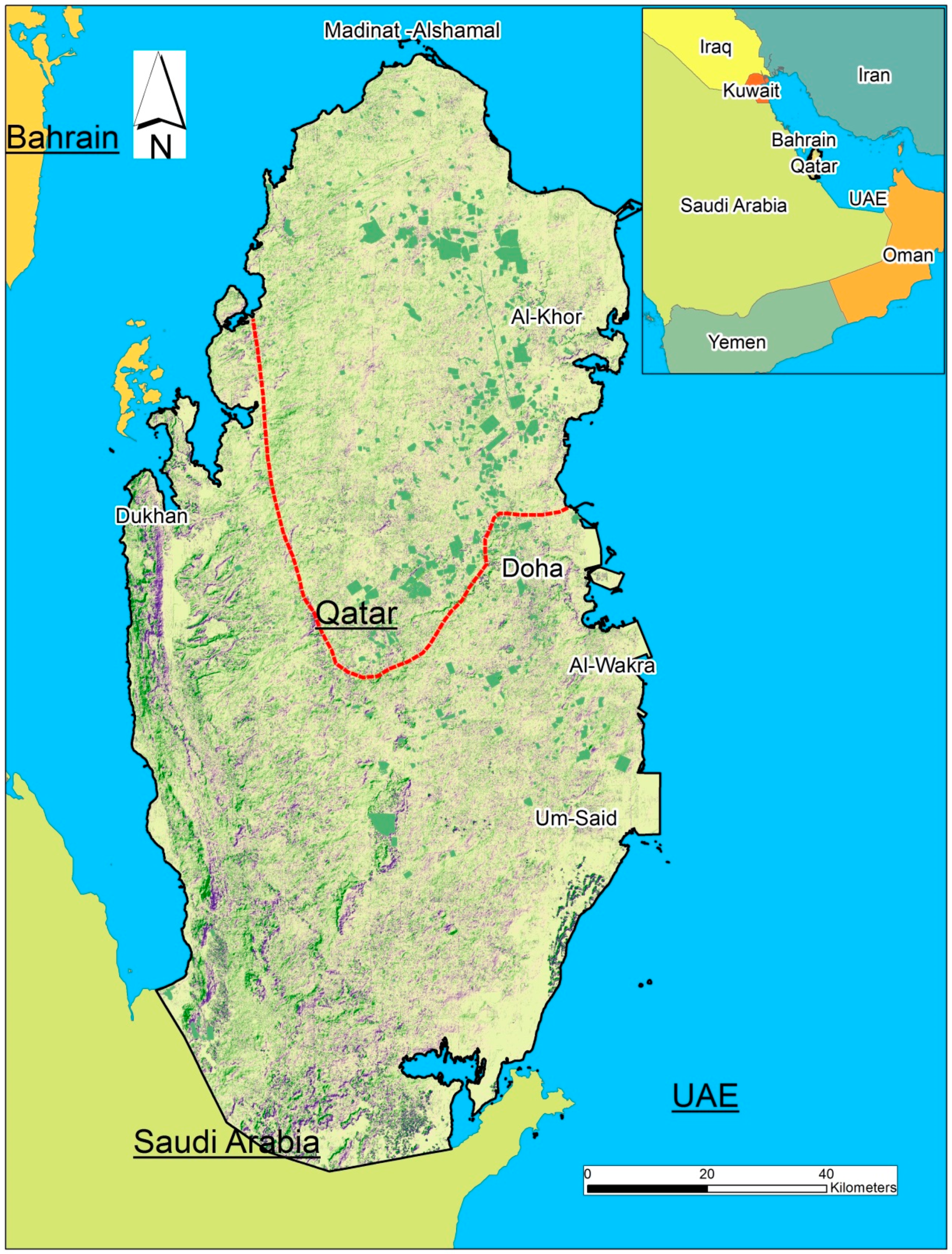
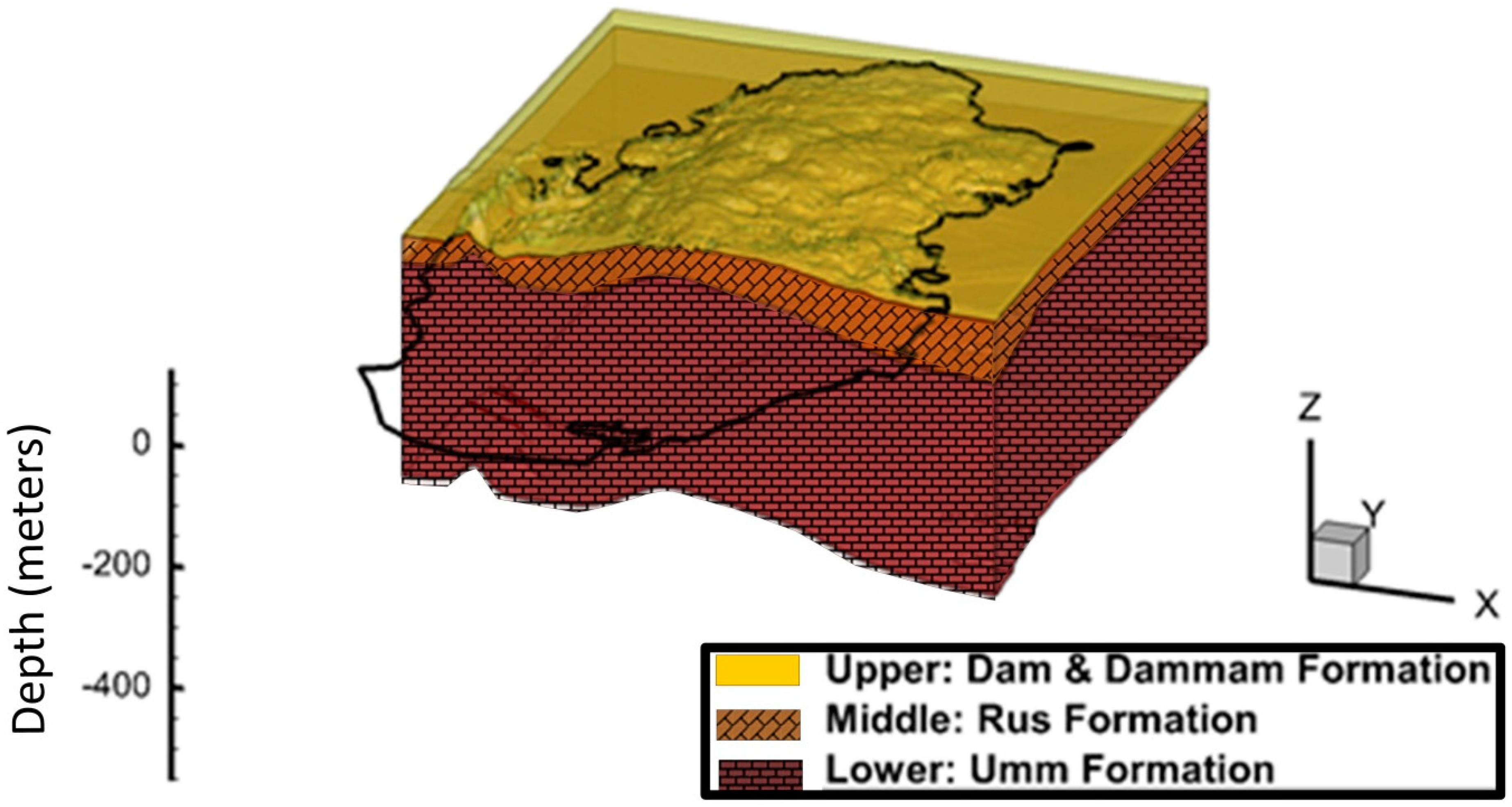
The area of study is the northern karst aquifer of Qatar (Figure 1). Qatar is located in the Arabian Peninsula, to the east of Saudi Arabia, with a total land area of 11,500 km2. The country is very arid, with no surface water and barely 80 mm of average annual rainfall [20]. The area of study covers approximately 4338 km2 and its geology comprises three layers of limestone and dolomite of Pliocene and Eocene age, namely the Dam and Dammam Formation, Rus Formation, and Um Al-Radhuma Formation (Figure 2). A thick layer of gypsum formation occurs within the Rus Formation and extends in many places over the southern aquifer. This has resulted in deterioration of the groundwater quality in the southern aquifer, compared to the north.
Qatar generally has a flat topography, except for some areas in the south. The country has a flat terrain as the topography varies between 0 near the coast to more than 100 m above the mean sea level in the south-west. Many land depressions occur in the country and vary in size between a few meters and more than one kilometer [21]. These land depressions are a result of land collapse due to the dissolution of the evaporate layer (gypsum) in the sub-surface and also due to cracks in the limestone at the top layer of geology. These land depressions are important for groundwater recharge. Rainfall-runoff accumulates in land depressions after heavy storms, eventually recharging the aquifer [22] and also enriching the soil by transporting fine sediments, making the depression suitable for agriculture [21].
The main aquifer occurs in Rus and Um Al-Radhuma Formation and is recharged through local rainfall. Thicknesses of the geological formations vary, as is shown in Figure 2, where thickness ranges between 50 m for the Dam and Dammam Formation to more than 300 m for the Um Al-Radhuma Formation [23]. A layer of gypsum (Evaporite unit) occurs within the Rus Formation, especially in the southern part of the country (Figure 2), but this layer is absent in the north. This explains why the groundwater quality is better in the north than the south.
The long term annual rainfall recharge is approximately 60 million m3 in the entire country [20,21,24]. Fresh groundwater occurs as lenses on the top of brackish and saline groundwater [25], especially in the northern part of the country, which receives the highest rainfall.
The aquifer has been extensively pumped over the last three decades, which has resulted in a significant drop in the water table and increase in salinity. Table 1 shows the groundwater abstraction from the aquifer for the period between 1976 and 2009 [26].
The conceptual model was built based on available data of groundwater levels [20] and a previous modelling study [24]. The model area covers the northern part of the country and is bounded by the Arabian Gulf from the east, north, and west. The southern boundary was considered as the head-dependent flow boundary.
The finite deference-based MODFLOW 2000 model was used to simulate the flow in the area [27]. The model grid contains 222 rows and 148 columns, with a regular grid size of 500 m in each direction. The model comprises one layer representing Rus and Um Al-Radhuma Formation. Top and bottom of the layers were identified based on structural contours of the geology [28] and bore-logs [20,21].
The east, north, and west boundaries are the sea, which was considered as a constant head boundary, whereas the southern boundary was considered as a head-dependent flow boundary. The General Head Boundary GHB module in MODFLOW was used to simulate the flow along the southern boundary. Flow values were estimated based on contour maps and previous modelling studies [24]. During the calibration process, the conductance value of the GHB was adjusted to decrease the error in the water budget [4].
The aquifer is highly heterogeneous as hydraulic conductivity varies significantly from one location to another. In general, hydraulic conductivity may vary between 0.01 m/day up to more than 100 m/day, due to the existence of fractures and conduits in the limestone [24]. The hydraulic conductivity values were later calibrated using the parameter estimation and uncertainty analysis software (PEST) with MODFLOW 2000 [14].
Groundwater recharge comes essentially from rainfall, which is too little. Despite the lower amount of rainfall, recharge occurs when heavy storms create enough runoff that accumulates in land depressions. Several studies have estimated rainfall recharge in Qatar [20,21,22,29,30]. From the previously-mentioned studies, it was found that rainfall recharge varies between 5 and 68 million m3 per year. In this study, the recharge spatial distribution is based on Baalousha et al. [22].
2. Model Calibration: PEST and Pilot-Points
The model was calibrated with PEST [14] using the truncated singular value decomposition “SVD-assist” [31], which is helpful in the case of high parameterization. By applying the SVD to the Jacobian matrix, super and sensitive parameters can be identified. Parameters with small eigenvalues can then be truncated. Kriging was used for interpolation of the parameter values obtained at the pilot-points.
The PEST calibration tool uses the least square method to minimize the difference between the model results and the observation measurements after applying weights to observations. The objective function is the squared sum of weighted residuals. The weights are assigned based on the uncertainty of field measurements; that is, measurements with high uncertainty have lower weights and vice versa.
The objective function φ of the inverse problem is based on the best fit between the linear combination of input parameters p, as affected by the model inputs X compared to observations h, is given by Doherty [14,32]:
where Q is a diagonal matrix of the squared observation and t indicates the transpose of the matrix. The weights and given by:
where m is the number of observations (i.e., targets), w is the weight of an observation point, and r is the residual. The weights vary depending on the relative importance of field data. In this study, all observations have been assigned an equal weight of 1 as all have the same importance.
As the inverse problem is ill-posed, PEST uses several tools to make it more stable. Regularization is one of these mathematical tools. PEST includes two types of mathematical regularization: one is Tikhonov regularization and the other is singular value decomposition—or SVD.
The Tikhonov regularization approach uses more information with the ill-posed inverse problem, such as suggesting a preferred value of the calibrated parameters. The SVD approach reduces the dimensionality of the problem by subtractions of parameters. The readers can refer to [4,5] for more details on regularization in PEST.
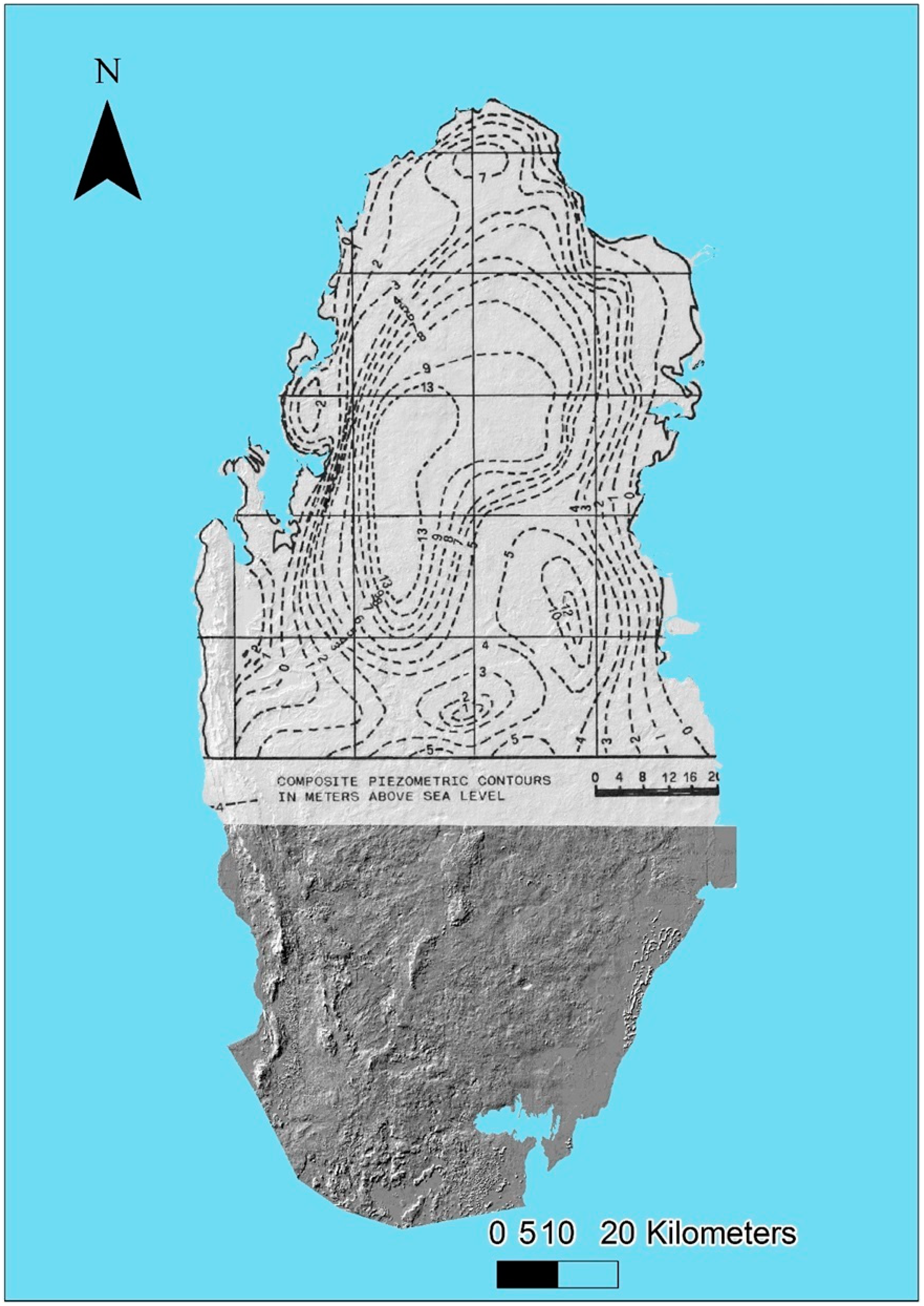
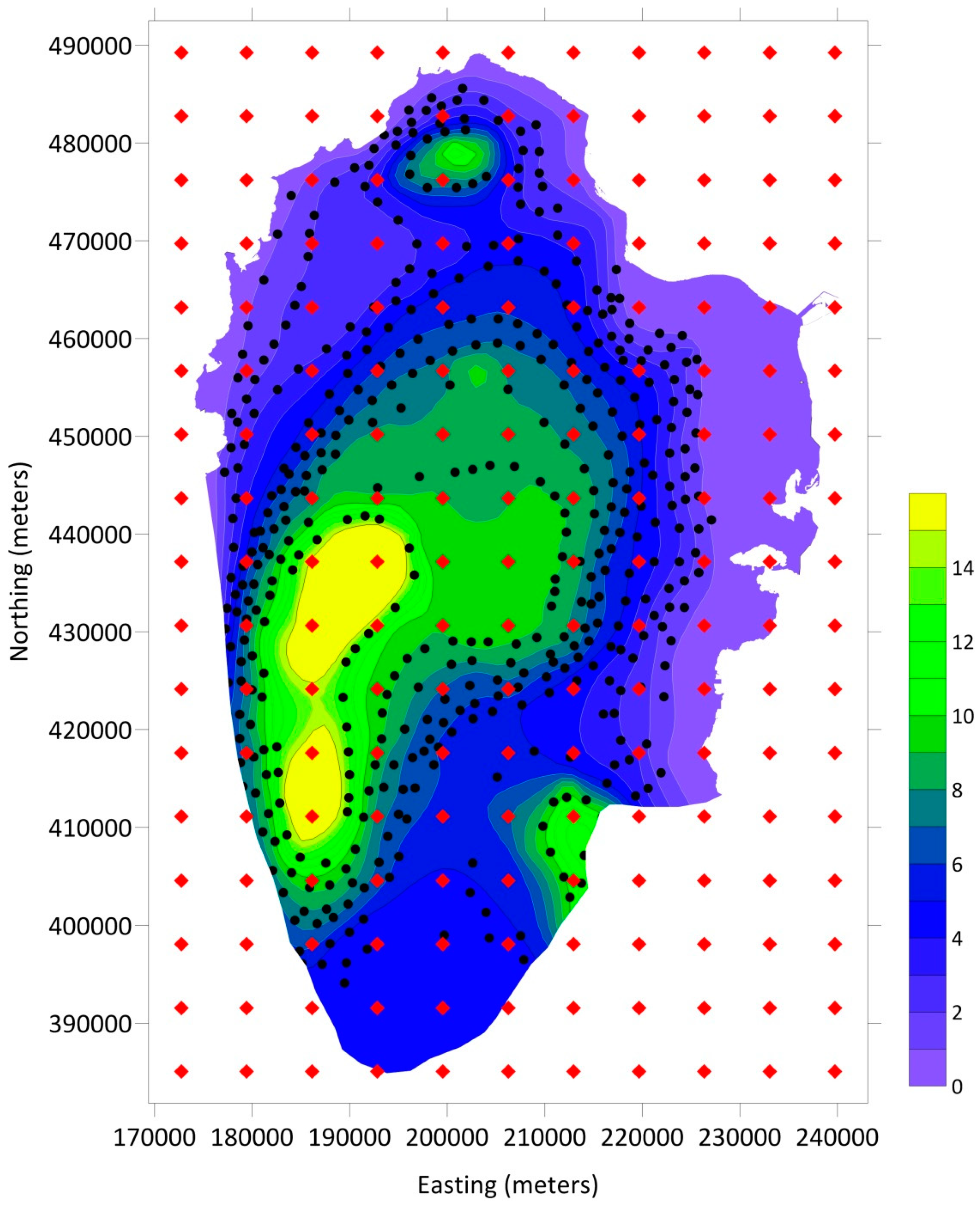
PEST minimizes the objective function until a pre-defined threshold error is achieved. The model was calibrated for steady state conditions using historical data of groundwater level. The calibrated parameter was the hydraulic conductivity. As the model has a steady state, the calibration targets are the groundwater head measurements in 1958, which is the oldest available data for the area of study (Figure 3). In this case, the threshold is the absolute mean residual head at any point that is less than 0.5. This value is considered adequate for model calibration given the uncertainty in the historical target heads values. It is assumed that the aquifer was in steady state conditions (or near steady state) because groundwater abstraction at that time was very low, and groundwater abstraction was little [24]. In the presumed steady state conditions in 1958, groundwater levels varied between 0.0 near the coastline to more than 13 m above the mean sea level in the central part of the aquifer. For calibration, groundwater level data from 1958 was used as observation points covering the entire model domain. As the uncertainty of this data is similar, all points had an equal weight in calibration.
3. Number of Pilot-Points
Three calibration sets with two configurations each were examined with different numbers of pilot-points. The number of pilot-points in the three runs was 112, 187, and 200 points, for the first, second, and third case, respectively. For each case, the model domain was divided into cells equal to the number of points. It should be noted that these cells are for pilot-points, not to be confused with the finite difference cells. Two configurations of pilot-points are considered: uniformly placed points in the centre of cells and random configuration were one point is randomly placed in each cell.
Statistical results of the three cases are shown in Table 2. As expected, when the number of pilot-points increases, so does the number of variables and the solution takes a longer time to be achieved (Equation (1)). In all cases, the threshold error (mean head residual < 0.5) was achieved, but the sum of squared weighted residuals varied. In the first case, random configuration (i.e., pilot-points = 112), the points were randomly placed in a grid of eight rows and 14 columns distributed over the model domain, thus the density was one pilot-point for every 72.8 km2. On the other hand, the uniform configuration of the first case implies placing the 112 points in the centres of the 112 cells. Given the low density of the points, the convergence was not easy, as fewer points were used for interpolation of the entire model domain. The sum of the squared weighted residual was 1370.
Mean Residual—Average error for the observations. This can be misleading because the positive and negative errors can cancel each other out. The root mean squared residual is calculated by calculating the square root of the average of the square of the errors for the observations. This tends to give more weight to cases where a few extreme error values exist.
In the second case (pilot-points = 187), the model domain was divided into a grid of 17 rows and 11 columns, thus the density of pilot-points is one point per 43.55 km2. As with the first case, uniformly distributed pilot-points produced less error than the randomly-distributed case. Although the mean residual head shows improvement from case 1, the sum of the squared weighted residual is significantly lower.
In the third case, the model domain was divided into a grid of 20 rows and 10 columns. The pilot-points density, in this case, is one per 40.8 km2. Obviously, this case shows much improvement compared to the previous two cases, as the number of pilot-points is higher. However, this came at a price of higher computational expenses.
4. Calibration Results
Based on the results shown in Table 2, it was clear the number of pilot-points of 187 (uniformly placed) is adequate for the calibration, as it converges easily with an error below the threshold value of 0.5 m. Therefore, 187 pilot-points were used to calibrate the model. As explained above, the pilot-points were defined using a grid of 17 rows and 11 columns created over the model domain. Each cell in this grid is 6700 m wide and has a height of 6500 m. The pilot-points were placed in the center of the defined cells (not to be confused with the finite-difference grid). Figure 4 shows the calibrated groundwater level for the steady state solution, with pilot-points and targets. The sum of squared weighted residual is 421 for the entire model area. The individual residuals at target points are within the acceptable threshold (i.e., the mean absolute residual of head at any point is less than 0.5 m), as shown in Table 2.
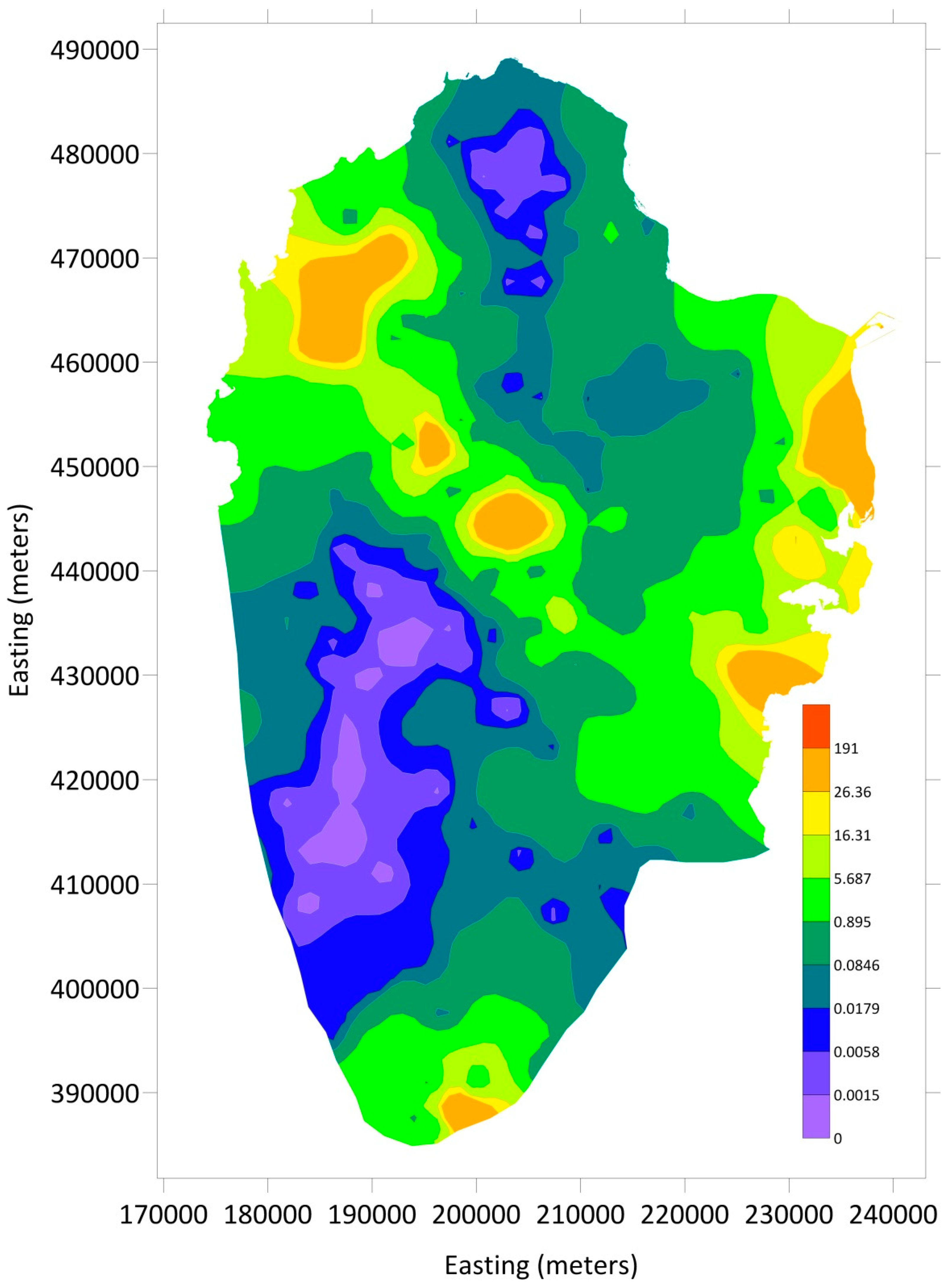
As depicted in Figure 5, values of the calibrated hydraulic conductivity vary between 0.001 and 191 m/day. While the majority of the model area shows low values (less than 10 m/day), a high hydraulic conductivity up to 191 m/day occurs in some locations. These locations occur in the east, north-west, south, and centre of the model area, as appears in Figure 5. This reveals the high heterogeneity of the aquifer due to karst features in some places.
5. Effect of Pilot-Points Locations
Two cases of pilot-points configurations were considered to investigate the effect of pilot-points locations on the calibrated hydraulic conductivity. These configurations are: randomly and uniformly spaced.
5.1. Random Perturbation
The same grid defined previously was used to generate the pilot-points (17 × 11 cells). Therefore, the total number of pilot-points is 187. In each square of this grid, one pilot-point was randomly placed, similar to Latin hypercube sampling. This results in stratified locations of pilot-points locations, which converges faster than random sampling [33,34,35] and covers the entire sampling domain.
5.2. Uniform Perturbation of Pilot-Points
As per the random placement, the model domain was divided into 17 rows and 11 columns. In each square, one pilot-point was placed at the same location within the square (same x and y within the square). The locations have been changed 20 times for the 20 runs of the model, keeping the distance increments between points constant.
6. Result and Discussion
To examine the effect of the locations of pilot-points on the estimated parameters, 20 runs were performed for each configuration of pilot-points locations (random and uniform distribution), respectively. Statistical analysis of the results was conducted, as well as a comparison between the uniform and random perturbation.
6.1. Random Placement
Twenty runs were performed using random realizations of the pilot-points in each run, as described above. In each run, the hydraulic conductivity was calibrated. In all cases, the calibrated absolute residual error was below the threshold value (<0.5). After all runs were completed, descriptive statistics of calibrated hydraulic conductivity were obtained to explore the effect of pilot-point locations on model calibration.
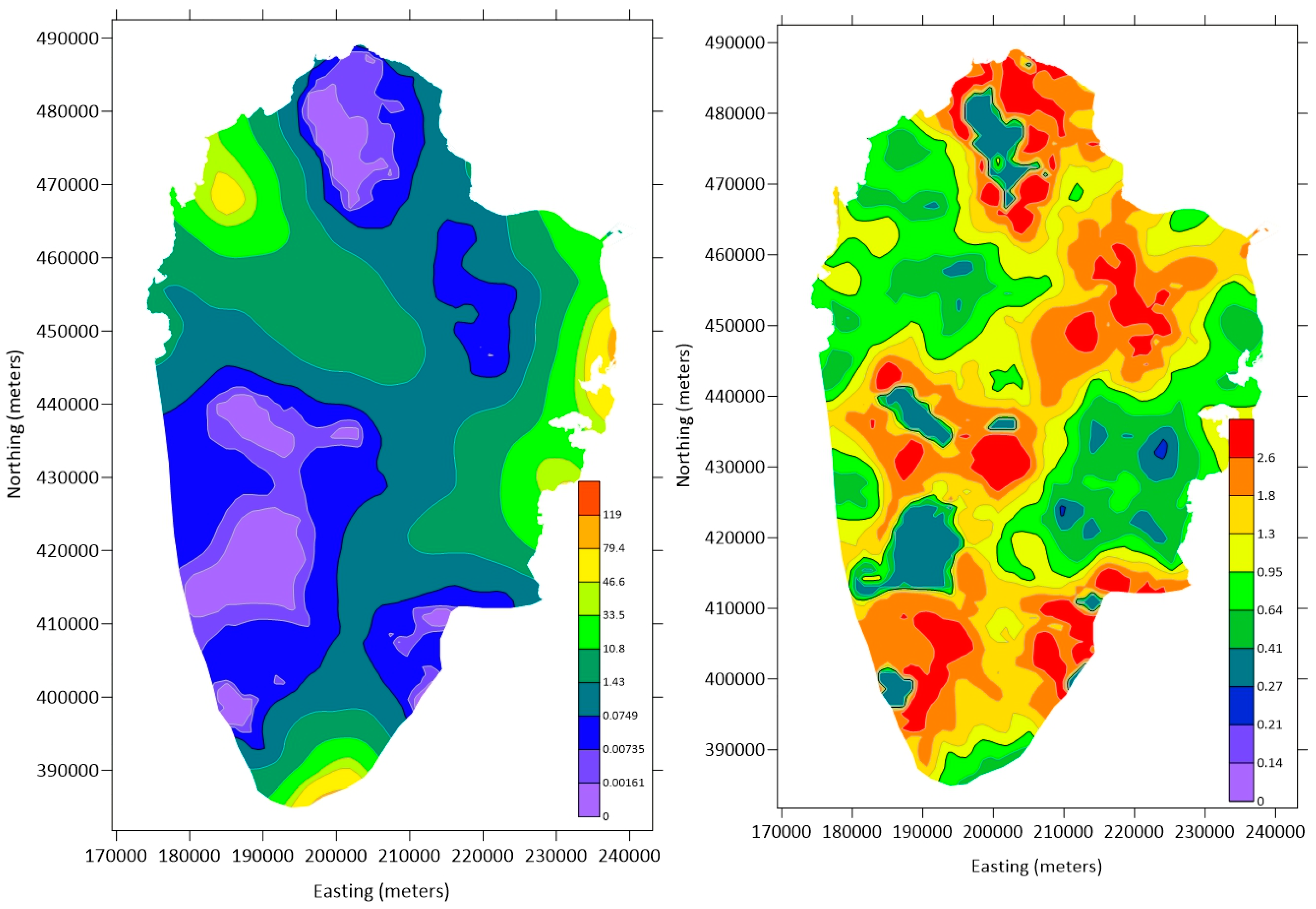
Figure 5 shows the calibrated model results, with 187 pilot-points centered at 187 cells. The calibrated hydraulic conductivity varies between 0.001 and 191.0 m/day. Figure 6 shows the mean value contour maps of the calibrated hydraulic conductivity and the coefficient of variation map resulting from the 20 runs. The coefficient of variation was used to show how the hydraulic conductivity values spread around the mean. It was obtained by dividing the standard deviation by the mean map. The mean value of the hydraulic conductivity resulting from these iterations varies between 0.001 and 118.8 m/day, which is lower than the initial results of the model (Figure 5). While the vast majority of the model domain has low conductivity (less than 10 m/day), areas of relatively higher hydraulic conductivity occur in the east and north-western area. Table 3 shows descriptive statistics of the mean and coefficient of variation of the hydraulic conductivity maps. The mean and median values of hydraulic conductivity are 9.58 and 1.4 m/day, respectively. The low median of the hydraulic conductivity is in line with the results of the pumping test [20], which show low values, except at some locations, where fractures/conduits occur.
6.2. Uniform Placement of Random Points
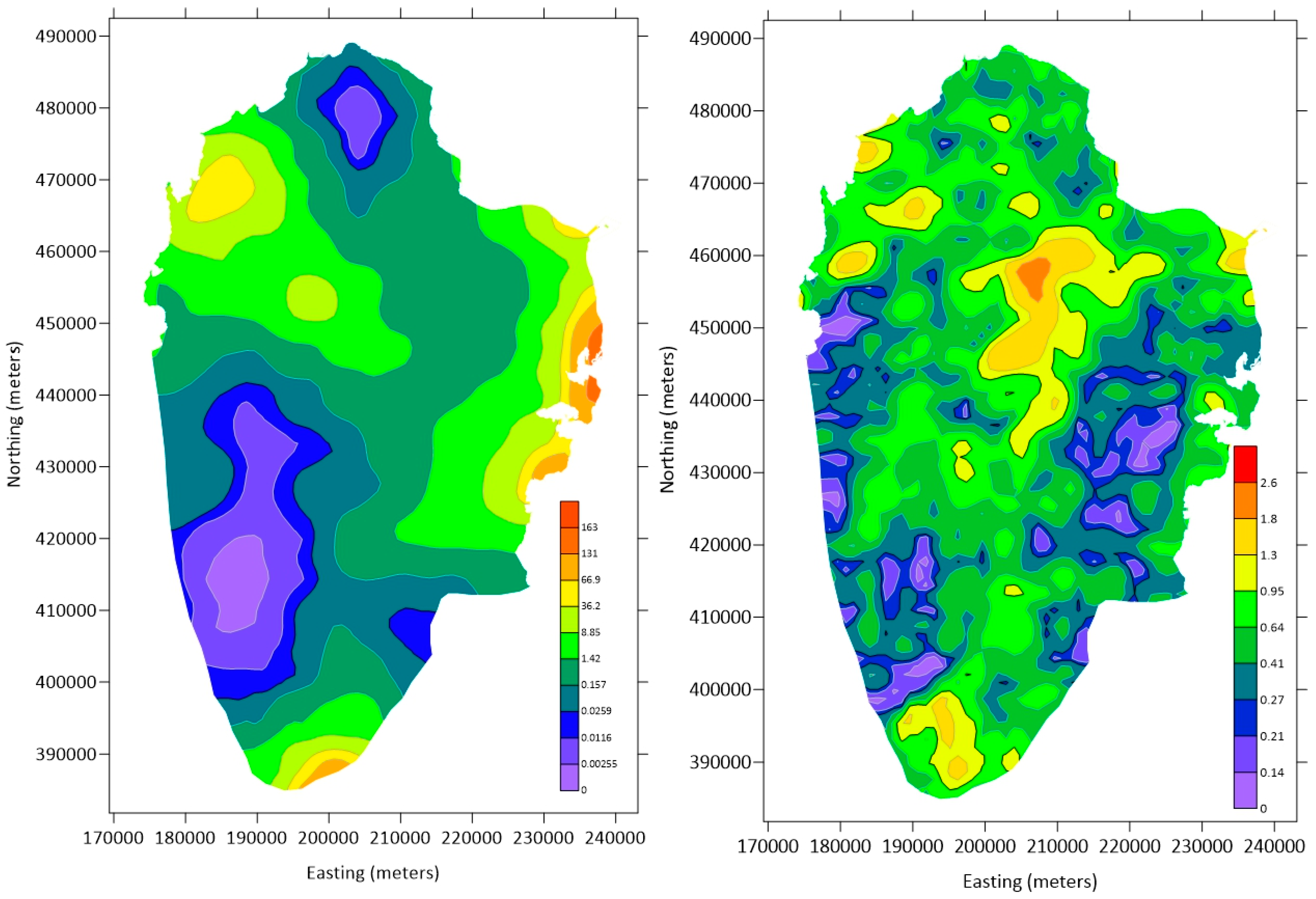
In the second case, another 20 runs were performed using uniformly placed pilot-points. In each run, pilot-points were distributed in a way that their locations are different, but the spacing between them is constant. Figure 8 shows the mean value map of the calibrated hydraulic conductivity using 187 pilot-points (the same number as in random placement). The map shows the mean of 20 runs using different perturbations of pilot-points and a uniform spacing between points. As with previous examples, the same threshold error was used. Descriptive statistics of both the mean and the coefficient of variation, in this case, are shown in Table 4. The hydraulic conductivity values vary between 0.001 and 162 m/day, with high values in the middle of the aquifer and in the north-west area. The coefficient of variation varies between 0.0 and 2.6.
Comparing the data in Table 3 and Table 4, while the median values are very similar in both cases, the mean of the uniformly distributed case is higher. From the minimum and maximum values, the uniform case data covers a wider range compared to the random case.
The statistics of the coefficient of variation maps show more similarity than the mean. The maximum values of the coefficient of variation are 3.6 and 3.4 for the random and uniform case, respectively. However, the uniform case shows less variance as the 99% tile is 2.6 compared with 3.4 in the case of random points. The mean and the median of the coefficient of variation are much lower in the case of uniform points than random points. Figure 6 and Figure 7 clearly show the similarity of the coefficient of variation in both cases, where high variations occur in the same areas. Unlike the random case, it is obvious that the coefficient of variation and the mean values in Table 4 are not similar.
6.3. Parameter Sensitivity Analysis
As part of PEST calculation, the Jacobian matrix is calculated as at least the number of calibration iterations plus one. The PEST calculates sensitivity with respect to each calibrated parameter. The Jacobian matrix contains the derivative of model output to the hydraulic conductivity in this case. Each column in the Jacobian matrix contains the derivative of the model output with respect to the calibrated parameter at each observation point. PEST calculates the composite sensitivity, which is the normalized magnitude of the Jacobian matrix columns with respect to the observation points. For any parameter i, the composite sensitivity (Si) is given by Doherty [14]:
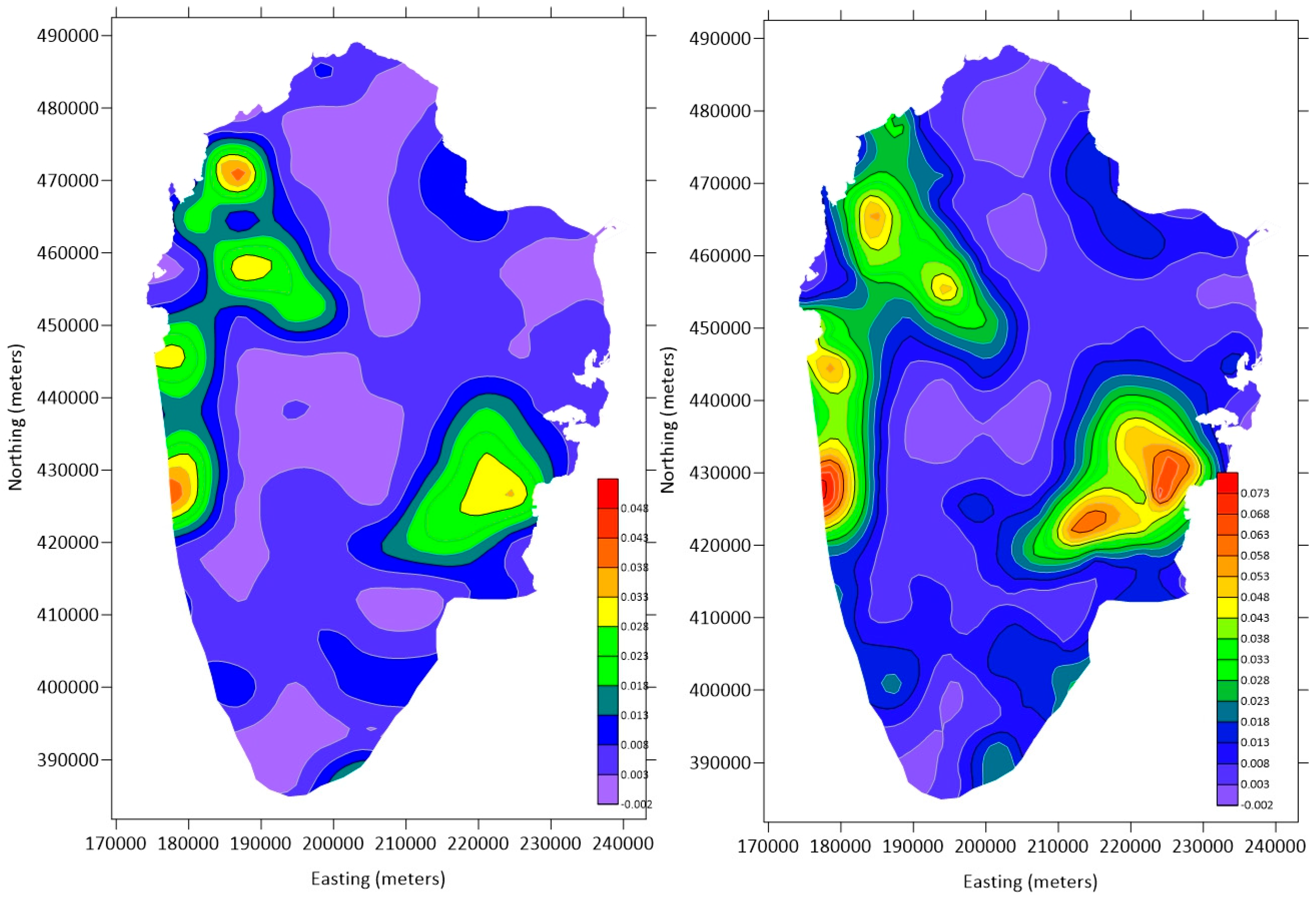
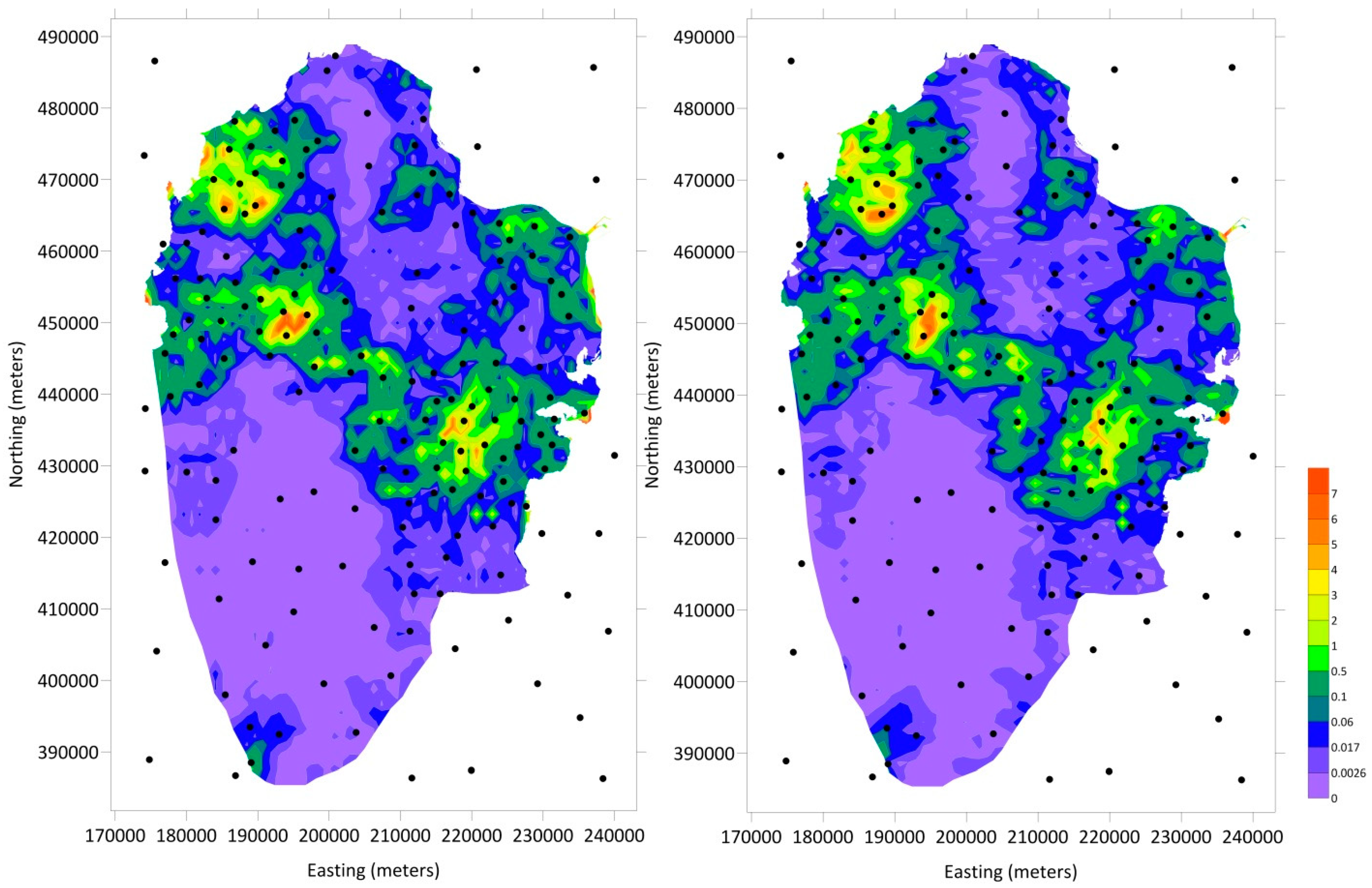
where J is the Jacobian matrix, Jt is the transpose of the Jacobian matrix, m is the number of observations, and Q is the weight matrix. In this study, Equation (3) calculates the sensitivity of the parameter value at each pilot-point normalized by the number of observation points (or targets) m. Figure 8 shows the mean composite sensitivity in the case of random and uniform pilot-points. While the general trend in sensitivity is similar in both figures, some differences exist. The random case shows a higher sensitivity magnitude than the uniform case. This is consistent with the high coefficient of variation for the case of randomly placed pilot-points. Composite sensitivity maps show that the model is more sensitive to parameter changes at pilot-points uniformly rather than randomly placed, with a maximum sensitivity of 0.048 and 0.073 for the random and uniform case, respectively.
6.4. Optimization of Pilot-Points Locations
Spatial interpolation depends on values at sampling points (in this case the pilot-points) and the spatial correlation between these points (in kriging). It is important to focus pilot-points at areas where the changes in the parameter under consideration are high (in this case high dk/dn, where n is the flow direction). In the steady state simulation, groundwater head is fixed. When calibrating both hydraulic conductivity and recharge, different solutions can be as long as the ration between recharge and hydraulic conductivity remains the same [36,37]. It is possible to estimate hydraulic conductivity if the recharge is well-known and vice versa [36].
For any given groundwater head, the spatial changes in hydraulic conductivity (dk/dn) are directly proportional to the spatial changes in the hydraulic head. The spatial changes in hydraulic conductivity (dk/dn) can be estimated from the piezometric map (Figure 3), and recharge R, using the continuity equation in both x and y directions:
where B is the thickness of the aquifer and h is the piezometric level. For the isotropic aquifer, Equation (4) can be rewritten as follows:
Raster maps were prepared using ArcGIS for the derivative of piezometric maps, aquifer thickness, and recharge. Using Equation (5), the derivative of estimated hydraulic conductivity (K) was obtained as shown in Figure 9. Although these maps are just an estimation, they provide a good indication of areas that need more pilot-points.
Pilot-points were redistributed on areas of high spatial variation of the estimated hydraulic conductivity. A total of 180 points were used, with a high density at a high spatial variation of the calibrated parameter and lower density elsewhere. Statistical analysis of the model calibration results using this configuration of pilot-points is shown in Table 5.
7. Conclusions
The northern aquifer of Qatar has a high variability in hydraulic conductivity as the aquifer is karst, but has a lower hydraulic conductivity in general. The calibrated hydraulic conductivity varies between 0.001 and 200 m/day. This study investigated the effect of pilot-points number, locations, and distribution on the model calibration results. It also explored the optimization of pilot-points locations for a steady state flow model.
Three calibration sets were performed using three different densities of pilot-points: one point per 72.8 km2, one point per 43.55 km2, and one point per 40.8 km2. It was found that the pilot-point density of one per 40.8 km2 provided the sought solution below the pre-defined threshold error, without over-parameterizing the inverse problem.
Two different perturbations of pilot-points were used; randomly and uniformly placed points, keeping the number of points constant in both cases (187 points or one per 43.55 km2). A total of 40 model calibrations were performed to test both configurations of pilot-points. The mean and the coefficient of variation of 20 runs for each case were obtained, with descriptive statistics.
Results show that the uniformly placed pilot-points perform better than the randomly placed points, given the same number of points. The randomly placed points solution has a higher coefficient of variation from the mean. This is because the interpolation between points is better when points are uniformly placed. The range of the calibrated parameter is higher in the case of uniform points. The uniformly placed points provide a good and unbiased coverage of the model area compared to randomly placed points. In both cases, high uncertainty (i.e., high coefficient of variation) occurs in the same areas.
In this study, and as the model represents a steady state, the relationship between hydraulic conductivity and recharge provided a means to estimate changes in hydraulic conductivity. This estimation can be used as a guide to place pilot-points at high variations of the hydraulic conductivity. Results demonstrated the usefulness of this method to optimize the pilot-points locations.
Author Contributions
Conceptualization, M.F.; Data curation, F.R.; Investigation, A.Y.; Methodology, H.M.B.
Funding
This paper was made possible by the NPRP grant # [NPRP 9-030-1-008] from the Qatar National Research Fund (a member of Qatar Foundation). The findings achieved herein are solely the responsibility of the author[s]. The publication of this article was funded by the Qatar National Library.
Conflicts of Interest
The authors declare no conflict of interest.
References
- Hayek, M.; Ackerer, P.; Sonnendrücker, É. A new refinement indicator for adaptive parameterization: Application to the estimation of the diffusion coefficient in an elliptic problem. J. Comput. Appl. Math. 2009, 224, 307–319. [Google Scholar] [CrossRef]
- Fahs, H.; Hayek, M.; Fahs, M.; Younes, A. An efficient numerical model for hydrodynamic parameterization in 2D fractured dual-porosity media. Adv. Water Resour. 2014, 63, 179–193. [Google Scholar] [CrossRef]
- Rajabi, M.M.; Ataie-Ashtiani, B.; Simmons, C.T. Model-data interaction in groundwater studies: Review of methods, applications and future directions. J. Hydrol. 2018, 567, 457–477. [Google Scholar] [CrossRef]
- Anderson, M.P.; Woessner, W.W.; Hunt, R.J. Applied Groundwater Modeling: Simulation of Flow and Advective Transport, 2nd ed.; Academic Press: London, UK; San Diego, CA, USA, 2015. [Google Scholar]
- Moore, C.; Doherty, J. Role of the calibration process in reducing model predictive error. Water Resour. Res. 2005, 41. [Google Scholar] [CrossRef]
- de Marsily, G. On the Calibration of Hydrologic Systems; Université Paris 6: Paris, France, 1978. [Google Scholar]
- LaVenue, A.M.; RamaRao, B.S.; De Marsily, G.; Marietta, M.G. Pilot Point Methodology for Automated Calibration of an Ensemble of Conditionally Simulated Transmissivity Fields: 2. Application. Water Resour. Res. 1995, 31, 495–516. [Google Scholar] [CrossRef]
- Doherty, J. Ground Water Model Calibration Using Pilot Points and Regularization. Ground Water 2003, 41, 170–177. [Google Scholar] [CrossRef]
- Alcolea, A.; Carrera, J.; Medina, A. Pilot points method incorporating prior information for solving the groundwater flow inverse problem. Adv. Water Resour. 2006, 29, 1678–1689. [Google Scholar] [CrossRef]
- Certes, C.; de Marsily, G. Application of the pilot point method to the identification of aquifer transmissivities. Advances in Water Resources, Parameter Identification in Ground Water Flow, Transport and Related Processes Part II-Advanced Applications. Adv. Water Resour. 1991, 14, 284–300. [Google Scholar] [CrossRef]
- RamaRao, B.S.; LaVenue, A.M.; De Marsily, G.; Marietta, M.G. Pilot Point Methodology for Automated Calibration of an Ensemble of conditionally Simulated Transmissivity Fields: 1. Theory and Computational Experiments. Water Resour. Res. 1995, 31, 475–493. [Google Scholar] [CrossRef]
- Lavenue, A.M.; de Marsily, G. Three-dimensional interference test interpretation in a fractured aquifer using the Pilot Point Inverse Method. Water Resour. Res. 2001, 37, 2659–2675. [Google Scholar] [CrossRef] [Green Version]
- LaVenue, A.M.; Pickens, J.F. Application of a coupled adjoint sensitivity and kriging approach to calibrate a groundwater flow model. Water Resour. Res. 1992, 28, 1543–1569. [Google Scholar] [CrossRef]
- Doherty, J. PEST Model-Independent Parameter Estimation User Manual Part I: PEST, SENSAN and Global Optimiser; Watermark Numerical Computing: Brisbane, Australia, 2019; 393p. [Google Scholar]
- Fienen, M.N.; Muffels, C.T.; Hunt, R.J. On Constraining Pilot Point Calibration with Regularization in PEST. Ground Water 2009, 47, 835–844. [Google Scholar] [CrossRef]
- Cooley, R.L. An analysis of the pilot point methodology for automated calibration of an ensemble of conditionally simulated transmissivity fields. Water Resour. Res. 2000, 36, 1159–1163. [Google Scholar] [CrossRef] [Green Version]
- Gómez-Hernánez, J.; Sahuquillo, A.; Capilla, J. Stochastic simulation of transmissivity fields conditional to both transmissivity and piezometric data—I. Theory. J. Hydrol. 1997, 203, 162–174. [Google Scholar] [CrossRef]
- Wen, X.-H.; Lee, S.; Yu, T. Simultaneous Integration of Pressure, Water Cut, 1 and 4-D Seismic Data In Geostatistical Reservoir Modeling. Math. Geol. 2006, 38, 301–325. [Google Scholar] [CrossRef]
- Klaas, D.K.S.Y.; Imteaz, M.A. Investigating the impact of the properties of pilot points on calibration of groundwater models: Case study of a karst catchment in Rote Island, Indonesia. Hydrogeol. J. 2017, 25, 1703–1719. [Google Scholar] [CrossRef]
- Schlumberger Water Services. Studying and Developing the Natural and Artificial Recharge of the Groundwater in Aquifer in the State of Qatar, Appendices; Schlumberger Water Services: Doha, Qatar, 2009. [Google Scholar]
- Eccleston, B.L.; Pike, J.G.; Harhash, I. The Water Resources in Qatar and Their Development; Food and Agricultural Organization of the United Nations: Rome, Italy, 1981. [Google Scholar]
- Baalousha, H.M.; Barth, N.; Ramasomanana, F.H.; Ahzi, S. Groundwater recharge estimation and its spatial distribution in arid regions using GIS: A case study from Qatar karst aquifer. Model. Earth Syst. Environ. 2018, 4, 1319–1329. [Google Scholar] [CrossRef]
- Kimrey, J. Proposed Artificial Recharge Studies in Northern Qatar; Open-File Report; United States Department of the Interior Geological Survey: Reston, VA, USA, 1985.
- Baalousha, H.M. Development of a groundwater flow model for the highly parameterized Qatar aquifers. Model. Earth Syst. Environ. 2016, 2, 67. [Google Scholar] [CrossRef]
- Lloyd, J.; Pike, J.; Eccleston, B.; Chidley, T. The hydrogeology of complex lens conditions in Qatar. J. Hydrol. 1987, 89, 239–258. [Google Scholar] [CrossRef]
- Baalousha, H.M.; Ouda, O.K.M. Domestic Water Demand Challenges in Qatar. Arab. J. Geosci. 2017, 10, 537. [Google Scholar] [CrossRef]
- Harbaugh, A.; Edward, B.; Mary, H.; Michael, M. MODFLOW-2000, The U.S. Geological Survey Modular Ground-Water Model-User Guide to Modularization Concepts and the Ground-Water Flow Process (Open-File Report No. 2000–92); US Geological Survey: Reston, VA, USA, 2000.
- Al-Hajari, S. Geology of the Tertiary and Its Influence on the Aquifer System of Qatar and Eastern Arabia. Ph.D. Thesis, University of South Carolina, Colombia, SC, USA, 1990. [Google Scholar]
- Harhash, I.E.; Yousif, A.M. Groundwater recharge estimates for the period 1972–1983; Ministry of Industry and Agriculture, Dept. of Agricultural and Water Research: Kingston, Jamaica, February 1985.
- Baalousha, H.M. Using Monte Carlo simulation to estimate natural groundwater recharge in Qatar. Model. Earth Syst. Environ. 2016, 2, 87. [Google Scholar] [CrossRef]
- Tonkin, M.J.; Doherty, J. A hybrid regularized inversion methodology for highly parameterized environmental models: Hybrid Regularization Methodology. Water Resour. Res. 2005, 41. [Google Scholar] [CrossRef]
- Doherty, J. PEST Model-Independent Parameter Estimation User Manual Part II: PEST Utility Support Software. Watermark Numerical Computing: Brisbane, Australia, 2019; 257p. [Google Scholar]
- McKay, M.D.; Beckman, R.J.; Conover, W.J. A Comparison of Three Methods for Selecting Values of Input Variables in the Analysis of Output from a Computer Code. Technometrics 1979, 21, 239. [Google Scholar] [CrossRef]
- Owen, A.B. Latin supercube sampling for very high-dimensional simulations. ACM Trans. Model. Comput. Simul. 1998, 8, 71–102. [Google Scholar] [CrossRef] [Green Version]
- Baalousha, H. Using Orthogonal Array Sampling to Cope with Uncertainty in Ground Water Problems. Ground Water 2009, 47, 709–713. [Google Scholar] [CrossRef] [PubMed]
- Luckey, R.; Gutentag, E.; Heimes, F.J.; Weeks, J.B. Digital Simulation of Ground-Water Flow in the High Plains Aquifer in Parts of Colorado, Kansas, Nebraska, New Mexico, Oklahoma, South Dakota, Texas, and Wyoming (No. Prof Pap 1400-D:57); US Geological Survey: Reston, VA, USA, 1986.
- Scanlon, B.R.; Healy, R.W.; Cook, P.G. Choosing appropriate techniques for quantifying groundwater recharge. Hydrogeol. J. 2002, 10, 18–39. [Google Scholar] [CrossRef]
Figure 1.
Qatar map showing the study area (the northern aquifer) and a regional map (inset). The red line shows the boundary of the north aquifer.
Figure 1.
Qatar map showing the study area (the northern aquifer) and a regional map (inset). The red line shows the boundary of the north aquifer.

Figure 2.
Schematic geological cross-sections in the north aquifer of Qatar.

Figure 3.
Piezometric map in 1958 used for calibration (modified after [21]), draped over the hill-shade model in the background.
Figure 3.
Piezometric map in 1958 used for calibration (modified after [21]), draped over the hill-shade model in the background.

Figure 4.
Calibrated groundwater level (meters above mean sea level) reproducing the piezometer map of 1958, pilot-points (red diamonds), and observations (black dots).
Figure 4.
Calibrated groundwater level (meters above mean sea level) reproducing the piezometer map of 1958, pilot-points (red diamonds), and observations (black dots).

Figure 5.
Calibrated hydraulic conductivity of the model using optimized location of 187 pilot-points (m/day).
Figure 5.
Calibrated hydraulic conductivity of the model using optimized location of 187 pilot-points (m/day).

Figure 6.
Mean value of the calibrated hydraulic conductivity from 20 simulations using random locations of pilot-points (left) and the coefficient of variation map (right) (m/day).
Figure 6.
Mean value of the calibrated hydraulic conductivity from 20 simulations using random locations of pilot-points (left) and the coefficient of variation map (right) (m/day).

Figure 7.
Mean value of the calibrated hydraulic conductivity from 20 simulations using uniform locations of pilot-points (left) and the coefficient of variation map (right) (m/day).
Figure 7.
Mean value of the calibrated hydraulic conductivity from 20 simulations using uniform locations of pilot-points (left) and the coefficient of variation map (right) (m/day).

Figure 8.
Mean composite sensitivity of model to changes in hydraulic conductivity values at pilot-points for the case of randomly placed points (left) and uniformly placed points (right).
Figure 8.
Mean composite sensitivity of model to changes in hydraulic conductivity values at pilot-points for the case of randomly placed points (left) and uniformly placed points (right).

Figure 9.
The spatial change in the estimated hydraulic conductivity in x-direction (left) and y-direction (right), and the new optimized pilot-points.
Figure 9.
The spatial change in the estimated hydraulic conductivity in x-direction (left) and y-direction (right), and the new optimized pilot-points.


Table 1.
Groundwater abstraction for the period between 1976–2009 [26].
Table 1.
Groundwater abstraction for the period between 1976–2009 [26].
| Year | Abstraction (million m3) | Year | Abstraction (million m3) |
|---|---|---|---|
| 1976 | 56.4 | 1993 | 179 |
| 1977 | 62 | 1994 | 209 |
| 1978 | 66.2 | 1995 | 240 |
| 1979 | 70.64 | 1996 | 258 |
| 1980 | 75 | 1997 | 265 |
| 1981 | 80 | 1998 | 260 |
| 1982 | 90.15 | 1999 | 263 |
| 1983 | 100.3 | 2000 | 272 |
| 1984 | 105 | 2001 | 255 |
| 1985 | 106.5 | 2002 | 250 |
| 1986 | 108.25 | 2003 | 248 |
| 1987 | 110 | 2004 | 249 |
| 1988 | 140 | 2005 | 248 |
| 1989 | 143.5 | 2006 | 237 |
| 1990 | 148 | 2007 | 238 |
| 1991 | 154 | 2008 | 239 |
| 1992 | 160 | 2009 | 248 |
Table 2.
Statistics for the calibrated model with 112, 187 and 200 points randomly and uniformly placed.
Table 2.
Statistics for the calibrated model with 112, 187 and 200 points randomly and uniformly placed.
| Statistics | 112 Points | 187 Points | 200 Points | |||
|---|---|---|---|---|---|---|
| Random | Uniform | Random | Uniform | Random | Uniform | |
| Mean residual head | −0.02 | 0.08 | 0.08 | −0.01 | 0.00 | 0.00 |
| Mean absolute residual head | 0.65 | 0.50 | 0.41 | 0.38 | 0.37 | 0.32 |
| Root mean squared residual head | 0.84 | 0.68 | 0.55 | 0.48 | 0.49 | 0.44 |
| Mean residual flow | 0.00 | 0.00 | 0.00 | 0.00 | 0.00 | 0.00 |
| Absolute residual flow | 0.00 | 0.00 | 0.00 | 0.00 | 0.00 | 0.00 |
| Root mean squared residual flow | −0.04 | 0.16 | 0.00 | 0.00 | 0.01 | 0.00 |
| Mean weighted residual (head and flow) | 1.27 | 0.98 | 0.89 | 0.71 | 0.72 | 0.62 |
| Root mean squared weighted residual (head and flow) | 1.64 | 1.33 | 1.05 | 0.92 | 0.96 | 0.86 |
| Sum of squared weighted residual (head and flow) | 1370 | 900.3 | 782.34 | 421.04 | 473.57 | 379.99 |
Table 3.
Descriptive statistics of the mean and the coefficient of variation maps of the hydraulic conductivity from 20 runs using randomly placed pilot-points.
Table 3.
Descriptive statistics of the mean and the coefficient of variation maps of the hydraulic conductivity from 20 runs using randomly placed pilot-points.
| Statistics | Mean Value Map | Coefficient of Variation Map |
|---|---|---|
| 1%-tile | 0.00087142857 | 0.361400126 |
| 5%-tile | 0.00160609005 | 0.390555544 |
| 10%-tile | 0.00735375552 | 0.577452325 |
| 25%-tile | 0.07488993856 | 0.901789639 |
| 50%-tile | 1.42516687096 | 1.308467642 |
| 75%-tile | 10.8043032033 | 1.869557044 |
| 90%-tile | 33.5103849654 | 2.48930949 |
| 95%-tile | 46.5985896143 | 2.929098095 |
| 99%-tile | 79.3751707193 | 3.415084443 |
| Minimum | 0.00087142857 | 0.234135821 |
| Maximum | 118.804007194 | 3.594438155 |
| Mean | 9.58889186912 | 1.44362254 |
| Median | 1.42653173771 | 1.308554766 |
Table 4.
Descriptive statistics of the mean and the coefficient of variation of hydraulic conductivity from 20 runs using uniformly placed pilot-points.
Table 4.
Descriptive statistics of the mean and the coefficient of variation of hydraulic conductivity from 20 runs using uniformly placed pilot-points.
| Statistics | Mean Value Map | Coefficient of Variation Map |
|---|---|---|
| 1%-tile | 0.002551672 | 0.14411592 |
| 5%-tile | 0.011559237 | 0.214720068 |
| 10%-tile | 0.025869756 | 0.274042945 |
| 25%-tile | 0.15722327 | 0.410987028 |
| 50%-tile | 1.422487888 | 0.641652186 |
| 75%-tile | 8.846138456 | 0.945805985 |
| 90%-tile | 36.22542187 | 1.338662571 |
| 95%-tile | 66.85036233 | 1.793603543 |
| 99%-tile | 131.2969591 | 2.558159718 |
| Minimum | 0.001391747 | 0.051191822 |
| Maximum | 162.747114 | 3.416383341 |
| Mean | 11.61371474 | 0.753418919 |
| Median | 1.423859795 | 0.641672875 |
Table 5.
Statistics of the calibrated model, using optimized locations of pilot-points.
| Statistics | Value |
|---|---|
| Mean residual head | 0 |
| Mean absolute residual head | 0 |
| Root mean squared residual head | 0 |
| Mean residual flow | 0 |
| Absolute residual flow | 0 |
| Root mean squared residual flow | 0 |
| Mean weighted residual (head and flow) | 0.03 |
| Root mean squared weighted residual (head and flow) | 0.56 |
| Sum of squared weighted residual (head and flow) | 319.54 |
© 2019 by the authors. Licensee MDPI, Basel, Switzerland. This article is an open access article distributed under the terms and conditions of the Creative Commons Attribution (CC BY) license (http://creativecommons.org/licenses/by/4.0/).
Share and Cite
MDPI and ACS Style
Baalousha, H.M.; Fahs, M.; Ramasomanana, F.; Younes, A. Effect of Pilot-Points Location on Model Calibration: Application to the Northern Karst Aquifer of Qatar. Water 2019, 11, 679. https://doi.org/10.3390/w11040679
AMA Style
Baalousha HM, Fahs M, Ramasomanana F, Younes A. Effect of Pilot-Points Location on Model Calibration: Application to the Northern Karst Aquifer of Qatar. Water. 2019; 11(4):679. https://doi.org/10.3390/w11040679
Chicago/Turabian StyleBaalousha, Husam Musa, Marwan Fahs, Fanilo Ramasomanana, and Anis Younes. 2019. "Effect of Pilot-Points Location on Model Calibration: Application to the Northern Karst Aquifer of Qatar" Water 11, no. 4: 679. https://doi.org/10.3390/w11040679
Note that from the first issue of 2016, this journal uses article numbers instead of page numbers. See further details here.